Abstract
A high-level control strategy for a quad rotorcraft Unmanned Aircraft System to perform trajectory tracking tasks is presented, which is based on a regressor-based adaptive approach. The high-level control is designed to interact with a low-level (internal) control loop that cannot be modified to suit the needs of academic researchers. Hence, the proposed control framework computes the appropriate high-level inputs for the inner controller, enabling the trajectory tracking task. The controller includes an integral action to overcome steady-state errors that may occur due to parameter estimation errors or constant disturbances. The stability of the equilibrium point is analyzed using Lyapunov theory, which shows that the tracking errors converge to zero and the parameter estimation errors remain bounded. The proposed control framework was tested on a real-time quad rotorcraft platform, and its performance was compared with four different control strategies. The results indicate that the proposed controller exhibits high accuracy and has better performance with respect to the other controllers.
1. Introduction
Among the different types of unmanned aerial vehicles, quadrotors became the most popular. There are many reasons for this: mechanical simplicity, compact size, maneuverability, vertical takeoff and landing, and hover are the most representative. Added to this, several applications have been found for them [1,2,3,4], and new ones will probably appear soon. Nevertheless, controlling such vehicles still represents a challenging task, especially considering their applications and the changing environments where they operate. Quadrotors are nonlinear underactuated systems with strongly coupled dynamics; hence, controllers must be able to ensure both stability and task accomplishment. Aiming to solve the trajectory tracking task of quadrotors, different control techniques have been employed [5,6,7,8,9,10,11].
1.1. Literature Review
Linear control schemes like proportional–integral–derivative (PID), H∞, linear quadratic regulator, and some others have been reported. Nonetheless, the development of linear controllers requires a simple approximation of the system dynamics, which neglects nonlinear aerodynamic phenomena. Thus, the real behavior of the quadrotor is not portrayed with fidelity. This is an issue for real outdoor applications where the environment interacts with the vehicle in uncertain ways and when the vehicle needs to perform tasks that require higher velocities. To overcome the aforementioned issues, nonlinear schemes have been employed to address the trajectory tracking task of quadrotors. For example, control algorithms based on feedback linearization, backstepping, model-based control, neural networks, and sliding mode control are reported in the literature. Many of the nonlinear schemes aim to provide robustness against parameter uncertainties, unmodeled dynamics, and external disturbances. However, only a few of them address the control of a quadrotor with an internal loop controller; the clearest examples of this are commercial quadrotors for recreational purposes. These platforms are mainly designed to be operated by a pilot. Owing to this condition, manufacturers include an inner controller that cannot be modified and which helps the pilot maintain the stability of the vehicle during the flying tasks. As discussed in [12,13,14], this fixed inner controller is not an impediment to employing them as platforms for testing control algorithms or even implementing them for real applications. These commercial platforms represent an affordable and economical option for actual implementation and experimental tests of controllers for quadrotors.
The works in references [15,16,17,18,19,20,21,22,23,24,25] addressed the control of a quadrotor under the assumption that an inaccessible and unmodifiable inner controller is present. Schemes such as inverse dynamic control, adaptive neural PID, cascade control, and adaptive generalized regression neural networks were introduced. In spite of the robustness of these controllers, some of the system parameters are required. To the best of the authors’ knowledge, regressor-based adaptive control has yet to be applied to a quadrotor equipped with an embedded controller. Thus, this is a novel regressor-based adaptive controller since an accurate knowledge of the system parameters is not needed and the control law is system-parameter-free. Additionally, in contrast with the neural network-based approaches, the proposed scheme is simpler and easier to implement.
1.2. Contribution
The contribution of this work is the development and design of an outer loop regressor-based adaptive controller for a quadrotor equipped with an inner loop controller to achieve trajectory tracking. In this regard, the procedure is performed in two major steps: First, similar to previous works [15,16,17,18,19,20,21,22,23,24,25], we assume the presence of an inaccessible and unmodifiable inner loop controller that not only guarantees internal stability but also allows one to transform the inputs from forces and torques to kinematic commands and represents the dynamics of the quadrotor as a general second-order system. Second, we design an outer loop controller directly on the already-obtained second-order system, thus achieving trajectory tracking and simplifying the analysis. As the outer loop is a regressor-based adaptive controller, the uncertainties coming from the inner loop are compensated in real time. In addition, the proposed outer loop scheme includes an integral action that increases the robustness of the controller and helps to cope with constant external disturbances. The proposed outer loop controller aims to provide a simpler adaptive solution in comparison with [24,25], which are more elaborated adaptive neural network-based controllers. Furthermore, the proposed scheme’s regression matrix is simpler in contrast to the proposed schemes in [19,21].
1.3. Organization and Notation
The organization of the document is the following. The dynamic model and the control objective are described in Section 2. In Section 3, the design and stability analysis of the proposed regressor-based adaptive controller are presented. The results of the experimental comparative study are shown in Section 4 and the conclusions are given in Section 5.
Notation: The notation adopted along this document is the following. is the Euclidean norm of the vector , given a symmetric positive definite matrix ; its minimum and maximum eigenvalues are denoted as and . stands for diagonal matrices with x in each diagonal element.
2. Preliminaries
2.1. Quadrotor Dynamic Model
The dynamic model of a quadrotor in the inertial reference frame is given as [24,25]
where (1) and (2) represent the position and attitude dynamics, respectively; is the cartesian position; is the attitude; is the mass of the vehicle; , with g being the gravitational acceleration constant; and are matrices that model the aerodynamic drag and damping effects, respectively; is the third column of matrix , which is a rotation matrix; is the inertia matrix; is the Coriolis matrix; is a transformation matrix; and and are the control inputs in the body reference frame. It is worth mentioning that representation (1)–(2) is valid for and , .
2.2. Inner Loop Controller
Based on [16,18,19,21,24,25,26], an inner loop controller serving as a stabilization system and acting as an intermediate between outer commands and the inputs of the quadrotor dynamic model is assumed to be
The parameters , , , , , , , , , and are strictly positive constants, and their physical meaning can be consulted in [25]. The variables , , , and are the inputs for the inner loop controller.
2.3. Quadrotor under Inner Loop Controller
In agreement with [16,18,19,21,24,25,26], the inner loop controller in (3)–(5) applied to dynamic models (1) and (2) leads to the second order system
where
contains the position in three-dimensional space and the yaw angle , and are positive definite diagonal matrices containing the parameters of the vehicle and the inner controller, explicitly given as
and
the matrix is a transformation matrix given by
and represents constant external disturbances that are bounded by with . Finally, the vector [24,25]
is a nondimensional input vector for the inner control loop with the following parameters:
- is an angular position command related to the displacement along the x-axis.
- is an angular position command related to the displacement along the y-axis.
- is a velocity command related to the displacement along the z-axis.
- is a velocity command related to the rotation around the z-axis.
A graphical representation of the quadrotor dynamics (1)–(2) under the inner loop controller (3)–(5), which result in (6), is provided in Figure 1.
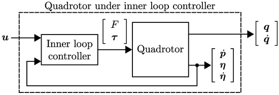
Figure 1.
Block diagram of a quadrotor with inner loop controller, which leads to system (6).
It is worth noticing that the inner loop controller given in Equations (3)–(5) is used only for demonstrative purposes, and any other inner loop controller can be used. In this sense, as long as the second-order system in Equation (6) is recovered, the proposed outer loop controller (presented in the next section) can be applied.
2.4. Control Objective
Let us assume that the matrices and in (8) and (9) are unknown, and the vectors in (7) and are available for measurement. Defining the trajectory tracking error as
and its derivative
where is defined in (7) and is the reference signal, which is assumed to be three times continuously differentiable. The objective is to design an outer loop controller so that the limit
is guaranteed.
3. Main Result
3.1. Outer Loop Design
The outer loop controller derivation is carried out for the system described in (6). The given outer loop scheme computes the required commands for the inner loop controller in order to achieve the objective (12).
Defining the variable
where is a positive definite diagonal matrix, the dynamics of the variable are given by
Assuming from (8), it holds that [25]
allowing one to multiply (14) by , obtaining
being , , and . Equation (15) is linearly parameterizable as follows:
where
is the vector containing the system parameters which is bounded as with , and
where
is the regression matrix.
In order to stabilize systems (13) and (16), the following regressor-based adaptive controller is proposed:
where and are positive definite diagonal matrices and is the estimation of the parameter vector , which is obtained through the following update law:
where is a positive definite diagonal matrix containing the adaptation gains. The dynamics of in (16) in a closed-loop with the proposed controller (17)–(19) is given by
where
is the parameter estimation error.
Notice that (20) can be rewritten as
where . Furthermore, recalling that is assumed to be constant and based on (18),
3.2. Convergence Analysis
The closed-loop system resulting from the dynamics of the quadrotor with an inner controller (6), the outer loop regressor-based adaptive controller (17)–(18), the update law (19), and the change in variable in (21)–(22) is given by
Notice that the origin is an equilibrium point of the overall closed-loop system (23).
Proposition 1.
Assume that matrices Γ and are selected such that the inequality
is satisfied.
Then, the equilibrium point is uniformly stable in the sense of Lyapunov. Moreover, the signals and are bounded, , and the limit (12) is fulfilled.
Proof.
Consider the following Lyapunov function candidate
which is globally positive definite, radially unbounded, and decrescent.
The time derivative of (25) is given by
By substituting the closed-loop dynamics in (23) into (26) and using the fact that
the following is obtained:
which can be rewritten as
where and
where is the identity matrix. Notice that (27) is always a negative function if Q is a positive definite matrix. In agreement with the Schur complement [27], Q is a positive definite matrix if and . This condition is satisfied with selected as in (24). Therefore, by fulfilling (24), is guaranteed to be a negative semidefinite function.
Based on Lyapunov’s method [28], we have that is a uniformly stable equilibrium point of the overall closed-loop system (23), which implies that , .
To assess the convergence of the error variables, consider the upper bound of (27), given by
Integrating both sides of (28), the following is obtained:
leading to sufficient conditions to invoke Barbalat’s lemma [28], concluding that as , implying that as as well, satisfying the control goal in (12). □
4. Experimental Results
The functionality of the proposed controller was demonstrated through an experimental test. Furthermore, its performance was assessed through comparison with other controllers reported in the literature. The comparison consists of achieving the trajectory tracking task. Four controllers were used in the comparison, an outer-loop PD scheme, a neural network-based scheme with integral sliding modes, an adaptive generalized regression neural network-based scheme, and an adaptive neural network-based scheme.
4.1. Benchmarking Platform
The benchmarking platform comprises two systems: a quadrotor and a motion capture system. The quadrotor employed in this work is s QBall 2 from Quanser® (Markham, ON, Canada), which is an off-the-shelf platform widely used in related research [24,25,29,30]. Figure 2 depicts a picture of the Qball 2. Figure 3 shows the motion capture system Optitrack® (Corvallis, OR, USA), which is employed to measure the cartesian position of the quadrotor and the yaw angle through an array of six Flex 3 cameras. Under this setup, the data are sent to a ground station through Wi-Fi. The benchmarking platform was configured and arranged in the same manner as in previous studies [24,25]. See [24,25] for a detailed description.
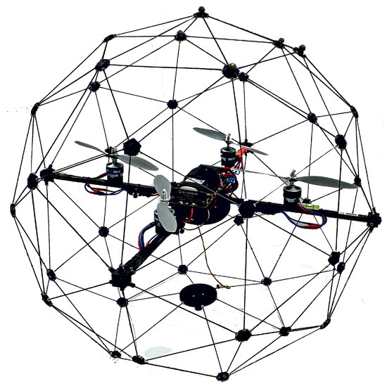
Figure 2.
Experimental platform: Qball 2 quadrotor from Quanser®.
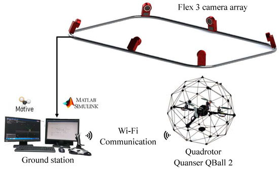
Figure 3.
Optitrack® motion capture system and communication protocol.
The parameters of the QBall 2 with the controller (3)–(5) are [24,25]:
All the tested controllers were implemented using MATLAB® R2014b and Simulink® 8.4 with a sample frequency of 500 [Hz].
4.2. Implemented Controllers
4.2.1. Outer Loop PD Controller
The performance of all the other tested schemes was evaluated based on the performance of the outer loop PD controller, which will be denoted hereafter as the PDC (PD controller). The PDC scheme is defined in [24] and was implemented using the gain matrices
4.2.2. GRNNC
A generalized regression neural network belongs to the category of radial basis function neural networks (RBFNNs) [31,32]. The generalized regression neural network-based controller hereafter denoted as GRNNC was introduced in [24]. The GRNNC scheme was implemented with the following gains
whose definitions are reported in [24].
4.2.3. ANNISMC
This controller was presented in [33] and was developed for the dynamic models in (1)–(2). Hence, it is not only an outer loop controller but has a two-loop configuration. In this scenario, controlling both position and attitude dynamics without access restrictions is possible. In this control scheme, the outer loop is an adaptive RBFNN scheme that governs the position dynamics and the inner loop is an integral sliding mode scheme that handles the attitude dynamics. This scheme will be referred to as ANNISMC (Adaptive neural network integral sliding modes control) in the remainder of this document. The ANNISMC was implemented using the following gains
The definition of each gain can be consulted in [24].
4.2.4. ANNC
This controller was introduced in [25], and it can be considered a PID-type controller with an adaptive neural compensation. The scheme is based on adaptive neural networks using the hyperbolic tangent function as an activation function. Similarly to [24], it computes the control inputs for an inner loop controller to achieve the trajectory tracking task. This scheme will be denoted as ANNC (adaptive neural networks controller) from now on in the document. The ANNC was implemented with the following gains
where the definition of each gain can be consulted in [25].
4.2.5. ARBC
4.3. Trajectory Tracking Task
The task concerns tracking an eight-shaped path while the height and the yaw angle remain constant. The following equations describe the desired trajectory:
where is the desired trajectory in the three-dimensional cartesian space. The paths obtained through the experimental tests for the PDC, ANNISMC, GRNNC, ANNC, and ARBC schemes are depicted in a three dimensional fashion in Figure 4. Additionally, a top view of the same paths showing the drawn trajectories along with the desired trajectory in the plane is given in Figure 5.
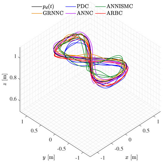
Figure 4.
Paths drawn by the quadrotor obtained with the tested controllers.
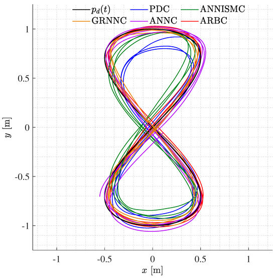
Figure 5.
Paths drawn by the quadrotor on the plane obtained with the tested controllers.
The tracking of each of the desired signals is shown in Figure 6, where it seems that the performance of all the tested schemes is similar, except for the PDC in the z coordinate and the yaw angle .
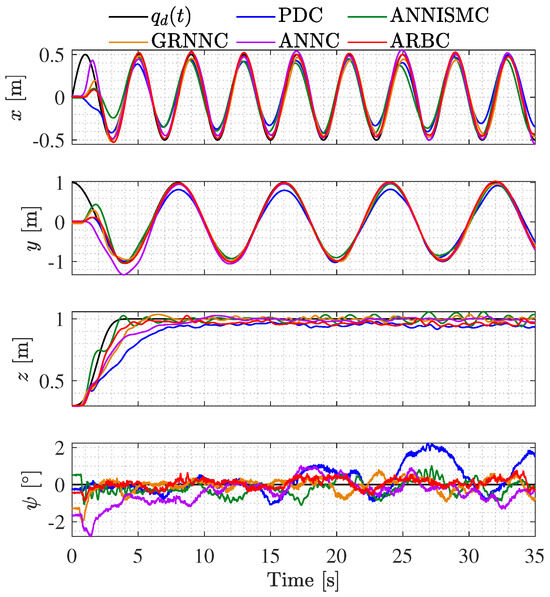
Figure 6.
Closed -loop system time response. Signals , , , and obtained with the tested controllers.
In Figure 7, the tracking errors obtained with the tested schemes are presented. It can be observed from it that the GRNN, ANNC, and ARBC have better performances than the PDC and ANNISMC in the x and y coordinates.
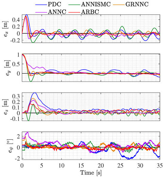
Figure 7.
Time response of the tracking error obtained with the tested controllers.
The obtained velocity errors are depicted in Figure 8. Notice that the closest to zero for the x, y coordinates and the yaw angle are the ones obtained with the ARBC.
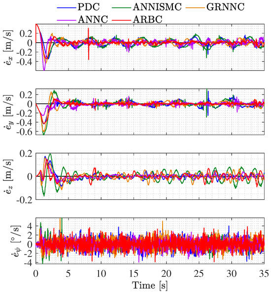
Figure 8.
Time response of the velocity error obtained with the tested controllers.
The provided control inputs by each controller are shown in Figure 9, these signals are the total thrust and the torques .
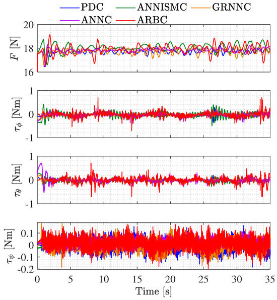
Figure 9.
Control input signals computed by the tested controllers.
The time evolution of the estimated parameters for the ARBC scheme during the trajectory tracking task are shown in Figure 10.
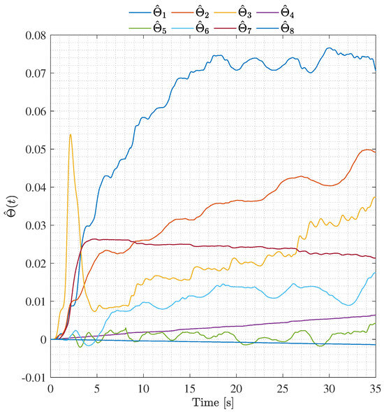
Figure 10.
Parameter estimation over time obtained with the ARBC algorithm.
The root mean square (RMS) value of and was computed in the time interval [s] to quantitatively assess the performance of all the tested controllers. Additionally, for every scheme, the relative percentage of improvement (PI%) was computed considering the performance of the PDC scheme as the comparison base point. Furthermore, the average of the PI% values regarding position and velocity errors was calculated. Table 1 presents the quantitative results, where the highest PI% values are in blue, and the lowest are in red. The values in blue mean that the performance on that specific feature was the best, while those in red mean that the performance was the worst. Although the ARBC scheme provided the best results for most features, it did not provided the best average results for position and velocity errors. It is worth mentioning that the ANNISMC, GRNNC, and ANNC schemes are all neural network-based schemes, while the ARBC is a regressor-based adaptive scheme with a much simpler structure and fewer parameters to be set up. Despite its simplicity, it significantly outperformed the other schemes in some features. These results indicate that with the ARBC scheme, a similar performance compared to other complex schemes can be achieved.

Table 1.
RMS values of and for all the tested controllers.
5. Conclusions
In this work, a regressor-based adaptive controller was introduced. The proposed scheme was developed as an outer loop scheme for a quadrotor that has an inaccessible and unmodifiable inner controller. The proposed controller was designed exploiting the structure of the dynamic model of the quadrotor with an inner controller. In addition, an integral action was included to overcome the steady-state error resulting from the parameter estimation error and constant disturbances. The stability analysis of the closed-loop system was presented, guaranteeing the fulfillment of the control goal and assuring the boundedness of the parameter estimation errors. An experimental comparative study regarding a PD scheme and other three neural network-based schemes was presented. The proposed scheme showed competitive performance since similar position and velocity errors compared to the tested controllers were obtained with it.
Author Contributions
Conceptualization, I.L.-S., J.M., L.R.G.C., A.D. and J.M.-V.; methodology, I.L.-S., J.M., L.R.G.C., A.D. and J.M.-V.; software, I.L.-S. and J.M.; validation, L.R.G.C., A.D. and J.M.-V.; formal analysis, I.L.-S. and J.M.-V.; investigation, I.L.-S., J.M., L.R.G.C., A.D. and J.M.-V.; data curation, I.L.-S. and J.M.-V.; writing—review and editing, I.L.-S. and J.M.-V.; visualization, I.L.-S.; supervision, L.R.G.C., A.D. and J.M.-V.; project administration, L.R.G.C., A.D. and J.M.-V.; funding acquisition, J.M.-V. All authors have read and agreed to the published version of the manuscript.
Funding
This research was funded in part by Consejo Nacional de Ciencia y Tecnología, CONACYT-Fondo Sectorial de Investigación para la Educación under Project A1-S-24762 and in part by Secretaría de Investigación y Posgrado-Instituto Politécnico Nacional, México. Proyecto Apoyado por el Fondo Sectorial de Investigación para la Educación.
Institutional Review Board Statement
Not applicable.
Informed Consent Statement
Not applicable.
Data Availability Statement
Data are contained within the article.
Conflicts of Interest
The authors declare no conflict of interest. The funders had no role in the design of the study; in the collection, analyses, or interpretation of data; in the writing of the manuscript; or in the decision to publish the results.
Abbreviations
The following abbreviations are used in this manuscript:
| ANNs | Adaptive Neural Networks; |
| ANNC | Adaptive Neural Network Control; |
| ANNISMC | Adaptive Neural Network Integral Sliding Mode Control; |
| ARBC | Adaptive Regressor-Based Control; |
| GRNNC | Generalized Regression Neural Network Control; |
| IMU | Inertial Measurement Unit; |
| NNs | Neural Networks; |
| PDC | Proportional-Derivative Control; |
| PID | Proportional–Integral–Derivative; |
| RBFNNs | Radial Basis Function Neural Networks; |
| RMS | Root Mean Square. |
References
- Chen, A.Y.; Huang, Y.N.; Han, J.Y.; Kang, S.C.J. A review of rotorcraft unmanned aerial vehicle (UAV) developments and applications in civil engineering. Smart Struct. Syst. 2014, 13, 1065–1094. [Google Scholar]
- Dupont, Q.F.; Chua, D.K.; Tashrif, A.; Abbott, E.L. Potential applications of UAV along the construction’s value chain. Procedia Eng. 2017, 182, 165–173. [Google Scholar] [CrossRef]
- Wang, N.; Ahn, C.K. Coordinated Trajectory-Tracking Control of a Marine Aerial-Surface Heterogeneous System. IEEE/ASME Trans. Mechatron. 2021, 26, 3198–3210. [Google Scholar] [CrossRef]
- Kourani, A.; Daher, N. Marine locomotion: A tethered UAV-buoy system with surge velocity control. Robot. Auton. Syst. 2021, 145, 103858. [Google Scholar] [CrossRef]
- Wang, N.; Su, S.F.; Han, M.; Chen, W.H. Backpropagating constraints-based trajectory tracking control of a quadrotor with constrained actuator dynamics and complex unknowns. IEEE Trans. Syst. Man Cybern. Syst. 2018, 49, 1322–1337. [Google Scholar] [CrossRef]
- Mo, H.; Farid, G. Nonlinear and adaptive intelligent control techniques for quadrotor uav—A survey. Asian J. Control 2019, 21, 989–1008. [Google Scholar] [CrossRef]
- Kim, J.; Gadsden, S.A.; Wilkerson, S.A. A comprehensive survey of control strategies for autonomous quadrotors. Can. J. Electr. Comput. Eng. 2019, 43, 3–16. [Google Scholar] [CrossRef]
- Wang, N.; Deng, Q.; Xie, G.; Pan, X. Hybrid finite-time trajectory tracking control of a quadrotor. ISA Trans. 2019, 90, 278–286. [Google Scholar] [CrossRef]
- Nguyen, H.T.; Quyen, T.V.; Nguyen, C.V.; Le, A.M.; Tran, H.T.; Nguyen, M.T. Control algorithms for UAVs: A comprehensive survey. EAI Endorsed Trans. Ind. Netw. Intell. Syst. 2020, 7, e5. [Google Scholar] [CrossRef]
- Nguyen, H.; Kamel, M.; Alexis, K.; Siegwart, R. Model predictive control for micro aerial vehicles: A survey. In Proceedings of the European Control Conference, Delft, The Netherlands, 29 June– 2 July 2021; pp. 1556–1563. [Google Scholar]
- Idrissi, M.; Salami, M.; Annaz, F. A Review of Quadrotor Unmanned Aerial Vehicles: Applications, Architectural Design and Control Algorithms. J. Intell. Robot. Syst. 2022, 104, 22. [Google Scholar] [CrossRef]
- Krajník, T.; Vonásek, V.; Fišer, D.; Faigl, J. AR-drone as a platform for robotic research and education. In Proceedings of the International Conference on Research and Education in Robotics, Prague, Czech Republic, 15–17 June 2011; pp. 172–186. [Google Scholar]
- Engel, J.; Sturm, J.; Cremers, D. Camera-based navigation of a low-cost quadrocopter. In Proceedings of the IEEE/RSJ International Conference on Intelligent Robots and Systems, Algarve, Portugal, 7–12 October 2012; pp. 2815–2821. [Google Scholar]
- Falcón, P.; Barreiro, A.; Cacho, M.D. Modeling of Parrot Ardrone and passivity-based reset control. In Proceedings of the 9th Asian Control Conference, Istanbul, Turkey, 23–26 June 2013; pp. 1–6. [Google Scholar]
- Santana, L.V.; Brandao, A.S.; Sarcinelli-Filho, M.; Carelli, R. A trajectory tracking and 3D positioning controller for the AR.Drone quadrotor. In Proceedings of the International Conference on Unmanned Aircraft Systems, Orlando, FL, USA, 27–30 May 2014; pp. 756–767. [Google Scholar]
- Santos, M.C.; Santana, L.V.; Martins, M.M.; Brandão, A.S.; Sarcinelli-Filho, M. Estimating and controlling UAV position using RGB-D/IMU data fusion with decentralized information/Kalman filter. In Proceedings of the IEEE International Conference on Industrial Technology, Seville, Spain, 17–19 March 2015; pp. 232–239. [Google Scholar]
- Santana, L.V.; Brandão, A.S.; Sarcinelli-Filho, M. Navigation and cooperative control using the AR.Drone quadrotor. J. Intell. Robot. Syst. 2016, 84, 327–350. [Google Scholar] [CrossRef]
- Santos, M.C.; Sarcinelli-Filho, M.; Carelli, R. Trajectory tracking for UAV with saturation of velocities. In Proceedings of the International Conference on Unmanned Aircraft Systems, Arlington, VA, USA, 7–10 June 2016; pp. 643–648. [Google Scholar]
- Santos, M.C.P.; Rosales, C.D.; Sarcinelli-Filho, M.; Carelli, R. A novel null-space-based UAV trajectory tracking controller with collision avoidance. IEEE/ASME Trans. Mechatron. 2017, 22, 2543–2553. [Google Scholar] [CrossRef]
- Rosales, C.; Rossomando, F.; Soria, C.; Carelli, R. Neural control of a Quadrotor: A state-observer based approach. In Proceedings of the International Conference on Unmanned Aircraft Systems, Dallas, TX, USA, 12–15 June 2018; pp. 647–653. [Google Scholar]
- Santos, M.C.P.; Rosales, C.D.; Sarapura, J.A.; Sarcinelli-Filho, M.; Carelli, R. An adaptive dynamic controller for quadrotor to perform trajectory tracking tasks. J. Intell. Robot. Syst. 2019, 93, 5–16. [Google Scholar] [CrossRef]
- Sarapura, J.A.; Roberti, F.; Toibero, J.M.; Sebastián, J.M.; Carelli, R. Visual Servo Controllers for an UAV Tracking Vegetal Paths. In Machine Vision and Navigation; Springer: Cham, Switzerland, 2020; pp. 597–625. [Google Scholar]
- Rubio Scola, I.; Guijarro Reyes, G.A.; Garcia Carrillo, L.R.; Hespanha, J.P.; Burlion, L. A Robust Control Strategy with Perturbation Estimation for the Parrot Mambo Platform. IEEE Trans. Control Syst. Technol. 2021, 29, 1389–1404. [Google Scholar] [CrossRef]
- Lopez-Sanchez, I.; Rossomando, F.; Pérez-Alcocer, R.; Soria, C.; Carelli, R.; Moreno-Valenzuela, J. Adaptive trajectory tracking control for quadrotors with disturbances by using generalized regression neural networks. Neurocomputing 2021, 460, 243–255. [Google Scholar] [CrossRef]
- Lopez-Sanchez, I.; Moyrón, J.; Moreno-Valenzuela, J. Adaptive neural network-based trajectory tracking outer loop control for a quadrotor. Aerosp. Sci. Technol. 2022, 129, 107847. [Google Scholar] [CrossRef]
- Santos, M.C.; Santana, L.V.; Brandão, A.S.; Sarcinelli-Filho, M.; Carelli, R. Indoor low-cost localization system for controlling aerial robots. Control Eng. Pract. 2017, 61, 93–111. [Google Scholar] [CrossRef]
- Zhang, F. The Schur Complement and Its Applications; Numerical Methods and Algorithms; Springer: Boston, MA, USA, 2006; Volume 4. [Google Scholar]
- Khalil, H.K. Nonlinear Systems, 3rd ed.; Prentice-Hall: Upper Saddle River, NJ, USA, 2002. [Google Scholar]
- Yang, P.; Liu, Z.; Wang, Y.; Li, D. Adaptive sliding mode fault-tolerant control for uncertain systems with time delay. Int. J. Autom. Technol. 2020, 14, 337–345. [Google Scholar] [CrossRef]
- Wang, B.; Shen, Y.; Zhang, Y. Active fault-tolerant control for a quadrotor helicopter against actuator faults and model uncertainties. Aerosp. Sci. Technol. 2020, 99, 105745. [Google Scholar] [CrossRef]
- Specht, D.F. A general regression neural network. IEEE Trans. Neural Netw. 1991, 2, 568–576. [Google Scholar] [CrossRef]
- Seng, T.L.; Khalid, M.; Yusof, R. Adaptive GRNN for the modelling of dynamic plants. In Proceedings of the IEEE Internatinal Symposium on Intelligent Control, Vancouver, BC, Canada, 30 October 2002; pp. 217–222. [Google Scholar]
- Li, S.; Wang, Y.; Tan, J.; Zheng, Y. Adaptive RBFNNs/integral sliding mode control for a quadrotor aircraft. Neurocomputing 2016, 216, 126–134. [Google Scholar] [CrossRef]
Disclaimer/Publisher’s Note: The statements, opinions and data contained in all publications are solely those of the individual author(s) and contributor(s) and not of MDPI and/or the editor(s). MDPI and/or the editor(s) disclaim responsibility for any injury to people or property resulting from any ideas, methods, instructions or products referred to in the content. |
© 2023 by the authors. Licensee MDPI, Basel, Switzerland. This article is an open access article distributed under the terms and conditions of the Creative Commons Attribution (CC BY) license (https://creativecommons.org/licenses/by/4.0/).