Abstract
Countless women and men worldwide have lost their lives to breast cancer (BC). Although researchers from around the world have proposed various diagnostic methods for detecting this disease, there is still room for improvement in the accuracy and efficiency with which they can be used. A novel approach has been proposed for the early detection of BC by applying data mining techniques to the levels of prolactin (P), testosterone (T), cortisol (C), and human chorionic gonadotropin (HCG) in the blood and saliva of 20 women with histologically confirmed BC, 20 benign subjects, and 20 age-matched control women. In the proposed method, blood and saliva were used to categorize the severity of the BC into normal, benign, and malignant cases. Ten statistical features were collected to identify the severity of the BC using three different classification schemes—a decision tree (DT), a support vector machine (SVM), and k-nearest neighbors (KNN) were evaluated. Moreover, dimensionality reduction techniques using factor analysis (FA) and t-stochastic neighbor embedding (t-SNE) have been computed to obtain the best hyperparameters. The model has been validated using the k-fold cross-validation method in the proposed approach. Metrics for gauging a model’s effectiveness were applied. Dimensionality reduction approaches for salivary biomarkers enhanced the results, particularly with the DT, thereby increasing the classification accuracy from 66.67% to 93.3% and 90%, respectively, by utilizing t-SNE and FA. Furthermore, dimensionality reduction strategies for blood biomarkers enhanced the results, particularly with the DT, thereby increasing the classification accuracy from 60% to 80% and 93.3%, respectively, by utilizing FA and t-SNE. These findings point to t-SNE as a potentially useful feature selection for aiding in the identification of patients with BC, as it consistently improves the discrimination of benign, malignant, and control healthy subjects, thereby promising to aid in the improvement of breast tumour early detection.
1. Introduction
As of the year 2020, breast cancer (BC) in women was the most common form of disease worldwide and the fifth leading cause of cancer deaths worldwide [1]. Overall, BC ranks as the fifth leading cause of death among women when all cancers are considered. Improvements and the availability of innovative screening technologies have increased effective prognosis and patient survival rates for BC over the past few decades [2,3]. Tumors are collections of dividing cells that grow to become masses of extra tissue; they can be malignant (cancerous) or benign. Breast tissue biopsies use a highly accurate method for detecting cancer [4]. Unfortunately, the biopsy procedure itself can be quite uncomfortable for the patients [5].
There has been a substantial development of technologies for BC detection throughout the years, including the use of image processing and analysis [5]. These cutting-edge methods allow doctors to better diagnose patients and provide better care. Radiologists can use images to detect irregularities and possible malignant tumors in the early stages of BC. Common methods for seeing breast tissue and detecting abnormalities include mammography, ultrasound, and magnetic resonance imaging (MRI) [6]. The mammogram is the method of choice for detecting BC [6]; this technique uses a two-dimensional (2-D) projection image of the breast for diagnosis. Details that are too small to be seen with the naked eye can be captured by these photos [7].
The use of images obtained from mammography and MRI for the purpose of diagnosing breast cancer offers a number of obstacles [5]. Although these imaging methods are essential for early diagnosis, they also come with a variety of drawbacks, such as the fact that mammography, despite its widespread application, may have limitations in terms of its sensitivity [8], particularly in women who have breast tissue that is dense. The MRI has a high sensitivity, but due to the fact that it is particularly sensitive to benign lesions, it can also lead to false positives [8]. Both mammography and MRI have the potential to provide false positive results, which can result in patients undergoing needless biopsies and experiencing emotional discomfort [9]. An overdiagnosis, in which benign tumours are identified and treated as dangerous, might result in overtreatment [9]. In addition, highly trained radiologists are required to appropriately interpret the results of mammograms and MRIs [10].
To prevent errors in diagnosis as much as possible, training and experience are absolutely necessary. In addition, cost and accessibility are important considerations, because an MRI scan can be rather expensive and may not be readily available to all individuals [8]. Because of this, its extensive usage in routine screening is restricted. In terms of data variability, the variability in image quality, location, and patient characteristics might affect the accuracy of both MRI-based detection methods and mammography-based detection methods [10,11,12].
In addition, image analysis tools have helped radiologists in image interpretation and BC detection, as these systems can be more successful and trustworthy in their diagnoses, because they make use of artificial intelligence to increase the accuracy of BC detection [5]. However, there are computational challenges to consider: the use of artificial intelligence for the analysis of the mammography and MRI images necessitate the collection of vast datasets for the purpose of training robust models; in addition, there is a concern regarding the models’ reliability and generalization [13].
Because blood and saliva hormones have the potential to serve as non-invasive and easily accessible biomarkers, using them in diagnostic laboratory testing can provide useful information regarding the diagnosis of breast cancer. Blood testing makes early diagnosis possible, which is helpful for people who are at higher risk. Biomarkers that can be found in saliva provide a patient-friendly way of collecting specimens, which enables the detection of cancer signals. Through the use of blood or saliva samples, laboratory tests determine hereditary risks, which in turn indicate hormone receptor status, which in turn influences treatment selections. This novel technique improves the ability to diagnose breast cancer in its earlier stages. Researchers choose drugs by monitoring changes in blood and plasma proteins, which can be found in the body. Methods for detecting breast cancer that are not intrusive and focused on the patient, such as using blood and saliva hormones, have been shown to be effective.
Therefore, the development of BC diagnostic methods that allow for early detection of the disease and that prompt treatment and recovery is crucial. In this study, we propose a machine-learning-based method for early BC detection [14]. Suitable features have been chosen in the proposed method by employing two-dimensionality reduction techniques such as factor analysis (FA) and t-stochastic neighbor embedding (t-SNE). To train and test their algorithms, the machine learning systems needed the right kind of data. By using a dataset with a good distribution for both training and testing, the models can improve their overall efficiency. The use of suitable features from the data can also improve the classification model’s performance. Therefore, improving model performance requires careful attention to data structure and feature selection. There has been some success in using the specific classifiers that are typically employed for classification-related problems to differentiate between people with BC and healthy individuals [5,7].
In this paper, the decision tree (DT), support vector machine (SVM) and k-nearest neighbors (KNN) modelas were evaluated using the collected statistical features, with FA and t-SNE serving as dimensionality reduction techniques methods. The Elwiya Oncology Teaching Hospital and the Center for Early BC Detection have generously donated their BC datasets for use in evaluating the effectiveness of the proposed system. Both the proposed method and the performance evaluation metrics have been validated via the k-fold cross-validation method.
The following are the most significant additions made by this work. Supervised learning has been used to examine significant hormones in theblood and saliva for accurate BC diagnosis. We found that combining blood biomarkers with the DT was an effective method for identifying BC.
Because blood and saliva hormones have the potential to serve as non-invasive and easily accessible biomarkers, using them in diagnostic laboratory testing can provide useful information regarding the diagnosis of breast cancer. Blood testing makes early diagnosis possible, which is helpful for people who are at higher risk. Biomarkers that can be found in saliva provide a patient-friendly way of collecting specimens, which enables the detection of cancer signals. Through the use of blood or saliva samples, laboratory tests determine hereditary risks, which in turn indicate hormone receptor status, which in turn influences treatment selections. This novel technique improves the ability to diagnose breast cancer in its earlier stages. Researchers choose drugs by monitoring changes in blood and plasma proteins, which can be found in the body. Methods for detecting breast cancer that are not intrusive and focused on the patient, such as using blood and saliva hormones, have been shown to be effective. Dimensionality reduction using the t-SNE method was also used in this investigation. FA and t-SNE were used in this study for the first time to differentiate between mild and severe cases of BC.
The purpose of using t-SNE is to preserve the local associations between points, which appear intuitively to be clustering rather than unrolling [15]. This is the motivation behind the usage of t-SNE; it is a non-linear dimensionality reduction strategy that focuses on keeping the structure of neighboring points [16]. It provides somewhat different outcomes each time on the same dataset, but these results are all focused on retaining the same information.
The t-SNE approach is a powerful dimensionality reduction technique that is used in data analysis to convert the high-dimensional Euclidean distances between data points into conditional probabilities that represent similarities [15]. Despite its stochastic nature, for several reasons, such as the preservation of local structures, the t-SNE is particularly effective at preserving local structures in high-dimensional data, as it focuses on maintaining the similarity relationships between data points, thereby making it useful for visualizing clusters and patterns that might be lost in other dimensionality reduction techniques such as principal component analysis (PCA) [17]. Moreover, t-SNE produces visually appealing embeddings that can help analysts and researchers interpret complex data [18]. Furthermore, t-SNE complements other dimensionality reduction methods such as PCA; it can be used to gain a more comprehensive understanding of the data [16]. Therefore, t-SNE’s ability to reveal local structures encourages researchers and analysts to often employ t-SNE alongside other techniques to uncover hidden patterns and gain a richer understanding of datasets.
Cancer is just one example of a disease where the symptoms do not appear until the disease has progressed to a later stage, at which point it is usually too late to treat effectively, thereby making early diagnosis crucial. Laboratory-based methods, such as blood and saliva tests with machine learning (ML) methods, are highly suitable for the detection of BC, because they circumvent the difficulties of invasive-based methods. Since blood tests are now often used to diagnose a variety of minor conditions, it would be great to be able to utilize them to diagnose major diseases such as cancer. Therefore, proper treatment and a full recovery depend on detecting BC at an early stage. Our objective was to conduct a comparative study to evaluate the blood and salivary levels of prolactin (P), testosterone (T), cortisol (C), and human chorionic gonadotropin (HCG) between breast cancer patients and healthy control subjects using ten statistical features with and without implementing dimensionality reduction techniques to discriminate the BC severity using data mining techniques.
2. Related Works
Many approaches have been proposed for diagnosing BC, but they all suffer from significant shortcomings when it comes to spotting the disease at an early stage [14]. Therefore, the job of clinical doctors is made more difficult by the fact that there are multiple factors to consider when making a diagnosis of BC. Diagnosing BC relies heavily on medical records and a system of expert judgment. All of these earlier proposals have aimed to diagnose BC in various ways. The downside to all of these methods is that they take longer to execute and have sub-par prediction accuracy. Better early detection is essential for effective treatment and a full recovery from BC, but the BC identification method’s prediction accuracy still needs work [5].
Low accuracy and lengthy computation times are thus major issues with the current approaches; these may be attributable to the inclusion of inappropriate features in the data. This calls for novel methods of BC detection to be implemented. It is a significant challenge and research gap to enhance the ML model’s prediction accuracy [5].
The dataset used is based on data from the University of Wisconsin’s database, which has seen extensive application in BC detection. To determine whether a tumor was benign or malignant in BC, Rashmi et al. utilized a naive Bayes classifier, which had an accuracy of 85% [19]. Breast cancer prediction accuracy has also been measured using the naive Bayes, C4.5 decision tree, and SVM classification algorithms by Pritom et al. There were a total of 35 data attributes that were gathered. By eliminating less important features, an effective feature selection method can boost a model’s accuracy [20]. In addition, using data on BC obtained from the Leiden University Medical Center, Guo et al. constructed a decision tree algorithm. The classifier was accurate for 70% of the time [21].
Lately, hormone tests using blood and saliva have emerged as a viable method in the detection of BC. Estrogen and progesterone are two hormones that play a significant role in the onset and progression of BC [22]. Increased levels of these hormones may be an early warning sign of sickness. Hormone analysis from saliva is a quick and easy way to check your hormone levels without any discomfort. Researchers can test for hormonal imbalances that may be related to BC by analyzing the samples of a patient’s saliva. Because it allows for routine screening and early intervention, this method may improve treatment outcomes for those at a higher risk of developing BC [23].
New techniques are constantly being developed, and the profession as a whole is expanding at a dizzying rate. In the future, we can anticipate even more precise and trustworthy approaches for breast cancer detection. Using a collection of clinical variables, Wang et al. [24] presented a data mining method for predicting breast cancer. The authors evaluated and contrasted the efficacy of four distinct data mining algorithms: the support vector machine (SVM), the artificial neural network (ANN), the naive Bayes classifier, and the AdaBoost tree. The SVM method was the most effective, with a success rate of 96.2%. Hosseini et al. [25] have employed three data mining methods, namely, k-nearest neighbours (KNN), the support vector machine (SVM), and random forest (RF), to predict breast cancer. The three algorithms were evaluated and compared using data from the Wisconsin Breast Cancer dataset. The RF algorithm was determined to have the highest accuracy (97.1%). Breast cancer recurrence has been analyzed using a data mining method that was proposed by Cesar et al. [26]. The authors implemented the decision tree, naive Bayes, and support vector machine data mining techniques on the Wisconsin Breast Cancer dataset. They observed that a 96.1% accuracy could be attained using the decision tree approach. Six data mining methods for detecting breast cancer were evaluated by Wassim et al. [27]. Decision trees, naive Bayes classifiers, support vector machines, random forests, k-nearest neighbors, and neural networks were some of the algorithms employed. The authors ran the data mining using the KNN algorithm, the NB algorithm, and the SVM, with the SVM having the best accuracy with a size of 97.07%.
In the context of breast cancer detection, there has been little research performed on laboratory tests that use blood and saliva as their primary ingredients. Li et al. have looked into the possibility of discovering new diagnostic biomarkers for breast cancer [28]. However, Sun et al. have used laboratory tests but did not expressly specify the use of hormones; they explored the function of diagnostic biomarkers in breast cancer diagnosis, which might potentially include hormonal indicators [29].
The diagnostic potential of saliva for systemic disorders was investigated in [30]. This review focused on the possible benefits of employing saliva as a diagnostic fluid, and it was suggested that these benefits could extend to the detection of hormone-related indicators in breast cancer [30].
The laboratory tests for breast cancer have been described as being able to be performed using either blood or saliva samples, which might include genetic tests that analyze an individual’s family history to estimate their likelihood of developing breast cancer [30]. It is essential to note that particular information about hormone markers in blood and salivary tests may require further inquiry to confirm their association with breast cancer; therefore, scientific literature and clinical studies are needed. Thus, in this study, an approach has been proposed for the early detection of BC by applying data mining techniques to the levels of prolactin (P), testosterone (T), cortisol (C), and human chorionic gonadotropin (HCG) in the blood and saliva.
3. Materials and Methods
Figure 1 shows the block diagram of the proposed method for BC severity identification from the hormonal level based on a blood and saliva dataset.
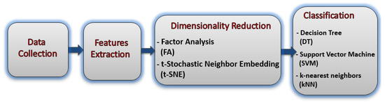
Figure 1.
The block diagram of the proposed study.
3.1. Data Collection Stage
This research was only carried out after receiving ethical approval from Elwiya Oncology Teaching Hospital and the Center for Early Breast Cancer Diagnosis. In addition, each participant gave their agreement after receiving appropriate information. The women who participated in the study were given complete information on all aspects of it, and they gave their consent to have their data published. In addition, when gathering our data, we made sure to conduct ourselves in accordance with the Declaration of Helsinki and its subsequent revisions. There were sixty individuals included in the dataset. (20 malignant, 20 benign, and 20 normal control individuals). Before enrolling in the study, participants who had a previous diagnosis of breast cancer were reviewed by an oncologist, and their participation was validated through clinical examination, breast biopsy, mammography, and ultrasound. Before any data were gathered, the goal of the study was explained to the participants, and they were given the chance to sign a consent form. Blood and saliva samples were used to compare levels of four hormones—prolactin (P), testosterone (T), cortisol (C), and human chorionic gonadotropin (HCG)—between breast cancer patients and the general population using data mining techniques. Table 1 Includes demographic characteristics such as age, body mass index (BMI), waist-to-hip ratio (WHR), types of blood groups, Lewis blood group, and the type of Fucosyltransferase 2 (FUT2) gene (secretor or non-secretor).

Table 1.
Socio-demographic information on the healthy control subjects and the malignant and benign patients. Age in years (mean ± standard deviation (SD)).
3.1.1. Blood Collection
About 5–10 mL of blood were aspirated using peripheral vein punctures and divided into 2 aliquots; the first one was transferred into EDTA tubes for direct determination of ABO blood group and also to determine the secretory status of subject according to Lewis blood group system. The second was dispensed in a plane tube (without anti-coagulant), and left for 15 min at 40 C to clot. Then, it was centrifuged at 3000 rpm for 10 min to collect serum, which was stored in −200 C until it was used for the determination of biomarkers.
3.1.2. Saliva Collection and Culturing
Saliva was collected from all subjects (after rinsing their mouth 2 times with cold drinking water 5–10 min prior to collection); about 3–5 mL of saliva was transferred into a sterile container. All samples were centrifuged at 3000 rpm for 10 min to eliminate any debris. The supernatant was divided into 2 aliquots; the first one was stored at −200 C until it was used for the determination of biomarkers, while the second aliquot was placed in a bath of boiling water for 10–15 min, and the boiled saliva was centrifuged at 3000 rpm for 2 min; we then removed the supernatant fluid, which was directly used to determine secretory status.
3.2. Features Extraction Stage
The foundation of the study is comprised of a collection of statistical information that is relatively comprehensive. The mean, variance, skewness, kurtosis, mode, median, minimum, maximum, summation, and range are the terms used to describe these characteristics [31]. A statistical features tool in Matlab 2022 was used to extract the statistical attributes from the raw dataset.
The dimension of the employed dataset’s feature matrix was (60 × 40), where (20 control + 20 benign + 20 malignant) = 60 observations, and the (10 features × 4 biomarkers (P, T, C, and HCG)) = 40 attributes.
3.3. Dimensionality Reduction Stage
The collected features from the preceding step size (60 × 10) for each of the four biomarkers (P, T, C, and HCG) must be further analysed before being applied to the classifier. Dimensionality reduction techniques must be used to reduce the challenges associated with a high-dimensional feature vector, which may result in the “curse of dimensionality”, as well as to reduce processing time. Dimensionality reduction strategies were used in this work to prevent classifier overloading, increase classification model precision, and reduce overfitting concerns. As a result, these algorithms must reduce the dimension of feature vectors to (30 × 4) for each of the four biomarkers (P, T, C, and HCG).
Our work on dimensionality reduction aimed to lessen the workload on the computer and free up storage space, all while experimenting with alternative data representations in the pursuit of better performance. We maintained consistency in the output data sizes across all of our experiments. The number of features was decreased in a series of experiments, and the resulting data was fed into a classifier.
3.3.1. Factor Analysis (FA)
Factor analysis (FA) is a statistical method for examining correlations by developing a set of underlying latent variables [32]. FA presupposes that the data can be initially organized according to the relationships between the variables. Strong relationships exist between the variables within a given group, but only weak relationships exist between variables in different groups. To this end, a factor may be represented by a single group, as is shown in Equation (1) [33].
where is the mean vector of all noticed samples , and is the factor loading matrix; is the Gaussian-distributed latent variable with its mean 0 being a zero vector and covariance matrix I being an identity matrix; the noise variables and form a diagonal matrix, with the diagonal elements being different.
When applied to the BC dataset, factor analysis will assist in identifying the underlying components that provide an explanation for the apparent variance in the data. The statistical method known as factor analysis can be used to perform the work of discovering latent variables that are responsible for explaining correlations between observable data. This effort can be accomplished by applying factor analysis. Utilizing factor analysis is one way to minimize the dimensionality of the data, which can be helpful in evaluating which elements of the BC are the most significant [33].
3.3.2. t-Stochastic Neighbor Embedding (t-SNE)
Features described by high-dimensional vectors or pairwise dissimilarities are embedded in a low-dimensional space while maintaining their neighbor identities using a probabilistic method called t-stochastic neighbourhood embedding (t-SNE) [15]. Overall, the t-SNE method involves centring a Gaussian on each object in the high-dimensional space and then using a small number of dissimilarities under this Gaussian to define a probability distribution over all of the possible neighbors of the features [16]. The conditional probabilities and will be equivalent for the map points and , respectively, that accurately model the similarity between the high-dimensional data points and , respectively. This insight serves as the inspiration for t-SNE, which seeks to identify a low-dimensional data representation that reduces the discrepancy between and . The Kullback–Leibler divergence, which in this instance equals the cross-entropy up to an additive constant, is a natural indicator of how accurately models . t-SNE employs a gradient descent technique to reduce the total of Kullback–Leibler divergences across all datapoints [15]. Equation (2) gives the cost function C.
Applying the t-SNE approach to the factor scores that were produced as a result of factor analysis will accomplish this. To visualize high-dimensional data in a low-dimensional setting, a non-linear dimensionality reduction method known as t-SNE may be applied. This method has the potential to be exploited. This is feasible due to the fact that t-SNE employs sparse networks in order to represent the data. The procedure of mapping the factor scores to a two- or three-dimensional space is what allows t-SNE to be of assistance in the process of locating patterns and clusters within the BC data. This can be done in any dimension.
3.4. Classification Stage
It was determined through an exhaustive study of the BC data that the individuals could be divided into three categories: normal, benign, and malignant. The quality of the generated features had a significant influence on the level of accuracy achieved by the classifier. As a consequence of this, the accuracy of the results of the classification can be affected not only by the techniques for dimensionality reduction that are selected, but also by the type of classifier that is utilized. In order to investigate BC differences based on emotional states, three classifiers were utilized: DT, SVM, and KNN.
The DT has a structure similar to a flowchart and is based on a set of rules; therefore, it is recognized to be very effective and provides clear guidance. This method begins at the very top with a question, which is also referred to as a “root node”. The algorithm works its way through the tree branches in a certain order, with each branch being determined by the responses to the questions that came before it until it reaches the leaf node, at which point it would indicate whether or not the individual is part of three leaf nodes that were malignant, benign, or part of the normal group [34].
DT is a supervised learning algorithm that needs labeled data to be trained. Labeled data would include patients with known diagnoses for normal, benign, or malignant classification. The DT approach is effective for classification. To avoid overfitting, pick parameters carefully. Additionally, the training set should be reflective of the data that the tree will classify. The Gini impurity and entropy are the main splitting criteria. The minimal number of samples in a leaf node before the tree can split is 50. This and the tree’s maximum depth avoid overfitting. Additionally, the DT classification tree model was applied here as well. It does this by using an algorithm for recursive partitioning, which produces nodes based on certain criteria for splitting the data. After the nodes have been produced and divided, they are used to grow a tree. In order to make use of the split criteria, it is necessary to locate the ideal split point. A function that is derived from the variance function is used to evaluate the splitting criteria’s overall level of quality. A function is used to analyze each possible split point, beginning with binary splits, and these determine which one provides the best results when compared to an optimization criterion. This allows the optimal point for splitting to be determined. In this particular body of work, Gini’s diversity index has served a role as an optimization criterion. The process of partitioning the instance space comes to an end when the classification tree reaches the pure node; a node is considered pure if it only contains observations that belong to a single class. The number 50 was used as the parameter in the DT method for classifying patients as normal, benign, or malignant [34].
For the SVM classifier, the optimizing C on the training set was selected to acquire the best results. To be more specific, the SVMs were trained for a variety of C values that fell within the range of in C values ranging from 0.0001, 0.001, 0.01, 0.1, 0, 10, 100, 1000, 10000. During the testing method, the result obtained for was the most favorable. For the purpose of implementing the multi-class SVMs classifier, the RBF–kernel functions were put to use. During the SVM training, the smoothing parameter was chosen based on the lowest mis-classification rate that was obtained from the training dataset. This was done so that the best possible model could be produced. The best value of can only be established by methodically experimenting with different values of during the various training sessions. As a result, the value of was changed between 0.1 and 1, with a step size of 0.1 between each change. At the value of , the rate of mis-classification was reduced to its lowest possible value.
Vapnik proposed the SVM based on computational learning theory [35]. In the field of engineering, SVM has found application in tasks such as classification, regression, and density estimation [36]. Even though SVM is primarily a classifier, it offers the flexibility to create linear classifiers by mapping input patterns into a higher-dimensional feature space. The main objective of SVM is to build hyper-planes that maximize the margin between classes while minimizing mis-classification errors [36].
In this research, the k value for the KNN classifier was chosen by varying k between 1 and 10 at intervals of 1. Maximum classification accuracy was achieved after training the classifier to determine the optimal value of k, which was found to be . Each experiment was categorized using KNN, with the Euclidean distance serving as the similarity metric.
The KNN algorithm is widely considered to be one of the non-parametric classification methods. The labels were assigned to samples in the training set by comparing their similarities. Specifically, it looks at the training observations in the significant features matrix to determine the classification [37,38,39,40]. The object is allocated to the class that has the highest frequency of occurrence among its k-nearest neighbors, where k is always a positive integer. When k > 1, KNN is more robust, and a bigger k value can assist to lessen the effect of noisy points in the training set [41,42,43]. The properties of the datasets generally dictate the parameter k, and the nearest samples are expected to contribute more than the far samples. The unknown sample belongs to a class that is shared by every KNN [44].
The classifier was prepared to locate the best estimation of k, which was obtained at k = 5, and to maximize the classification accuracy. The Euclidean distance was utilized as a similarity measure to classify each trial using the KNN. The presentation of the proposed framework was assessed by utilizing average classification accuracy.
The best results for the classifiers were obtained by carrying out a 5-fold cross-validation (CV). This procedure was carried out, and the average of the 5 folds was then reported. During this procedure, the entire dataset was split up into a (24 × 4) training set and a (6 × 4) testing set. This was done so that the accuracy of our overall results could be improved as a result. The performance of the proposed framework was evaluated by using the average classification precision, sensitivity, specificity, accuracy, and F1-score, which were reported as a percentage, and the confusion matrix made it possible to classify the BC severity. The confusion matrices were produced for each classifier while doing a 5-fold cross-validation (CV), in which the final confusion matrix was obtained by averaging the 5 folds.
4. Results
Learning patterns from data, feature extraction, and dimensionality reduction let a model or classifier make judgements, especially in complicated tasks such as BC categorization. This study trained DT, SVM, and KNN models on labeled data. The models learned feature–label patterns during training. The model performance was robustly performed via cross-validation. Finally, the model was evaluated on a new dataset to determine its real-world performance. This stage determines if the model overfit (learned noise in the training data) or underfit (failed to capture patterns). Overfitting can be prevented by splitting the dataset into several smaller sub-sets (folds)—keeping one fold aside for testing purposes while training the model on the remaining four folds. These procedures were performed five times, and the model’s efficacy on the unseen fold was assessed using the selected metric (precision, sensitivity, specificity, accuracy, and F1-score). Finally, a single performance score for the model was calculated by averaging the performance of the used metrics throughout all five iterations.
The authors of t-SNE have conceded that, depending on the starting point and other random factors, the algorithm may return different results despite using the same data and parameters. Thus, we have used a fixed random seed to guarantee that the process always began in the same place. Thirty iterations were performed. As a result, the algorithm should eventually reach a more robust answer. To solve the reproducibility problem of t-SNE, it is recommended to run the algorithm five times with different random seeds and to then take an average of the results so that the classification results are not skewed due to overfitting. In order to further analyze the data, it was split into five independent datasets of similar sizes. We used one of these sub-sets as our test data, and we used the other nine to train our classifier. Five iterations of this process yielded ten reliable results. The accuracy of this dataset’s 5-fold CV was determined by averaging these results. This intended to lessen the effect of chance and to lead to more consistent outcomes. The features were first calculated using the training set to create the input features vector for t-SNE. After that, dimensionality reduction was accomplished by computing both the training and testing sets.
The effectiveness of the blood hormones in normal, benign, and malignant subjects was demonstrated through the use of performance assessment criteria such as precision, sensitivity, specificity, accuracy, and F1-score for the DT, SVM, and KNN classifiers, as is shown in Table 2.
Table 2.
Performance evaluation, including precision, sensitivity, specificity, accuracy, and F1-score for the DT, SVM, and KNN classifiers to show the blood hormones performance from normal subjects, benign patients, and malignant patients.
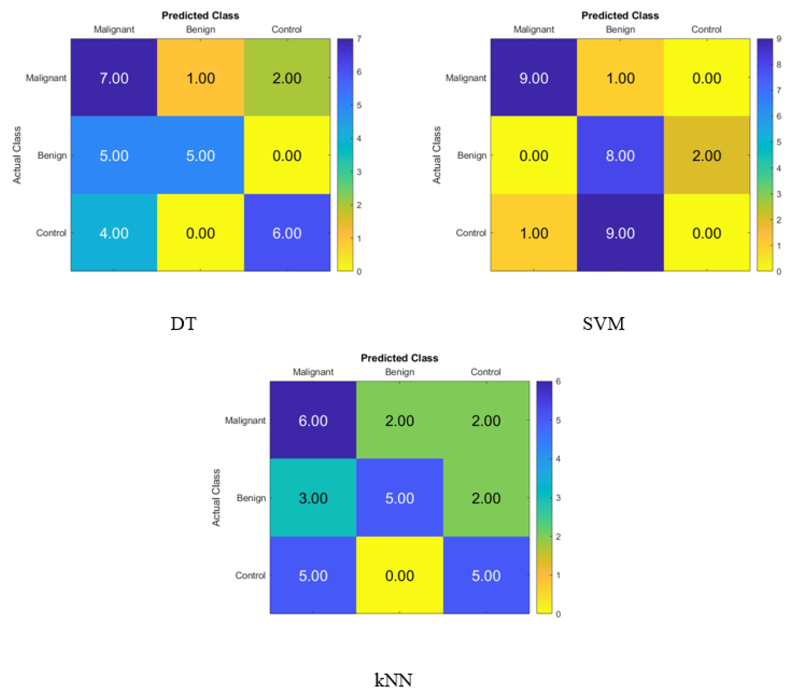
Figure 2 displays the confusion matrix for normal subjects’, benign patients’, and malignant patients’ identification from the blood levels of P, T, C, and HCG using statistical features and KNN, SVM, and DT classifiers, respectively. The correct recognition is observed on the diagonal, whereas the off-diagonal represents the substitution errors. The percentage of correctly classified data from the DT, SVM, and KNN classifiers utilizing the blood level hormones is shown in Figure 2. The DT’s accuracy was 60%, the SVM’s was 56.67%, and the KNN’s was 53.33%. Hence, using the DT, six of the control patients, five of the benign patients, and seven of the malignant patients were properly identified, whereas three of the malignant were incorrectly classified as one benign patient and two control healthy subjects. Moreover, five of the benign patients were incorrectly classified as malignant patients, and four of the control subjects were incorrectly classified as malignant patients.
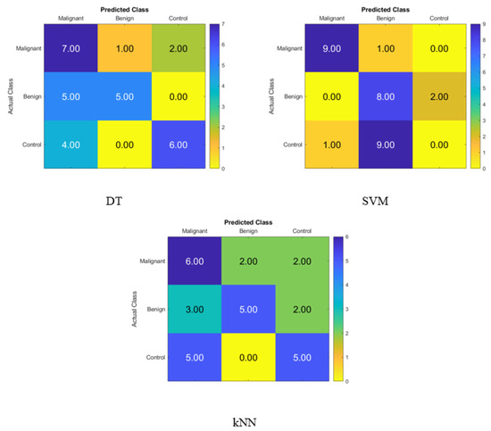
Figure 2.
Confusion matrices for the DT, SVM, and KNN classifiers to demonstrate the blood hormones performance from the normal subjects, benign patients, and malignant patients.
Table 3 shows the effectiveness of the blood hormones in normal, benign, and malignant subjects demonstrated through the use of performance assessment criteria such as precision, sensitivity, specificity, accuracy, and F1-score for the DT, SVM, and KNN classifiers using the FA dimensionality reduction technique.
Table 3.
Performance evaluation, including precision, sensitivity, specificity, accuracy, and F1-score, for the DT, SVM, and KNN classifiers using the FA dimensionality reduction technique to show the blood hormones performance from normal subjects, benign patients, and malignant patients.
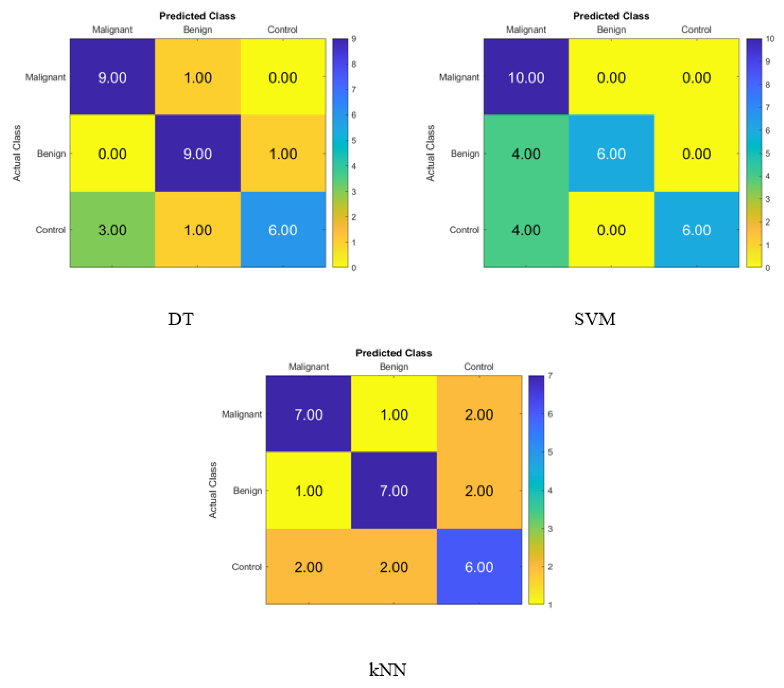
The confusion matrix for identifying normal subjects, benign patients, and malignant patients based on the blood levels of P, T, C, and HCG is depicted in Figure 3, and it was created with statistical features after applying the FA dimensionality reduction techniques with the KNN, SVM, and DT classifiers with FA in that order. On the diagonal, the correct recognition is seen, whereas the off-diagonal areas represent the incorrect substitutions.

Figure 3.
Confusion matrices for the DT, SVM and KNN classifiers using FA dimensionality reduction technique to demonstrate the blood hormones performance from the normal subjects, benign patients, and malignant patients.
Figure 3 displays the percentage of correctly identified data produced by the DT, SVM, and KNN classifiers with FA using blood level hormones. The accuracy of the DT, SVM, and KNN was 80%, 73.33%, and 66.67%, respectively. As a result, nine of the malignant patients, nine of the benign patients, and six of the control subjects were correctly identified using the DT, whereas one of the malignant patients was incorrectly classified as a benign patient. Moreover, one of the benign patients was incorrectly classified as a malignant patient, and four of the control subjects were incorrectly classified as three malignant patients and one benign patient.
Table 4 shows the effectiveness of the blood hormones in normal, benign, and malignant subjects demonstrated through the use of performance assessment criteria such as precision, sensitivity, specificity, accuracy, and F1-score for the DT, SVM, and KNN classifiers using the t-SNE dimensionality reduction technique.
Table 4.
Performance evaluation, including precision, sensitivity, specificity, accuracy, and F1-score, for the DT, SVM, and KNN classifiers using the t-SNE dimensionality reduction technique to show the blood hormones performance from normal subjects, benign patients, and malignant patients.
After applying the t-SNE dimensionality reduction techniques to the KNN, SVM, and DT classifiers, the confusion matrix is shown in Figure 4 for identifying normal people, benign patients, and malignant patients from the blood levels of P, T, C, and HCG using statistical characteristics. In the diagonal, we see accurate recognition, whereas the off-diagonal areas represent substitution mistakes. Figure 4 depicts the proportion of correctly categorized data from the DT, SVM, and KNN classifiers by applying t-SNE to the blood level hormones. The accuracy of the DT was 93.3%, of the SVM was 86.7%, and of the KNN was 73.3%. Thus, the DT correctly identified 10 control patients, 10 benign patients, and 8 malignant patients, whereas 2 of the malignant patients were incorrectly classified as control healthy subjects.
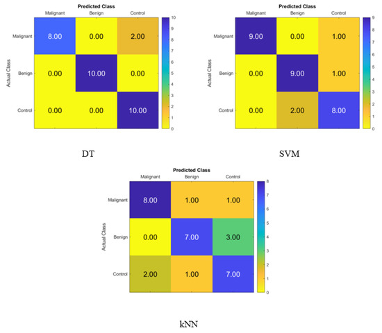
Figure 4.
Confusion matrices for the DT, SVM, and KNN classifiers using the t-SNE dimensionality reduction technique to demonstrate the blood hormones performance from the normal subjects, benign patients, and malignant patients.
Table 5 shows the effectiveness of saliva hormones in normal subjects, benign patients, and malignant subjects demonstrated through the use of performance assessment criteria such as precision, sensitivity, specificity, accuracy, and F1-score for the DT, SVM, and KNN classifiers.
Table 5.
Performance evaluation, including precision, sensitivity, specificity, accuracy, and F1-score, for the DT, SVM, and KNN classifiers to show the saliva hormones performance from normal subjects, benign patients, and malignant patients.
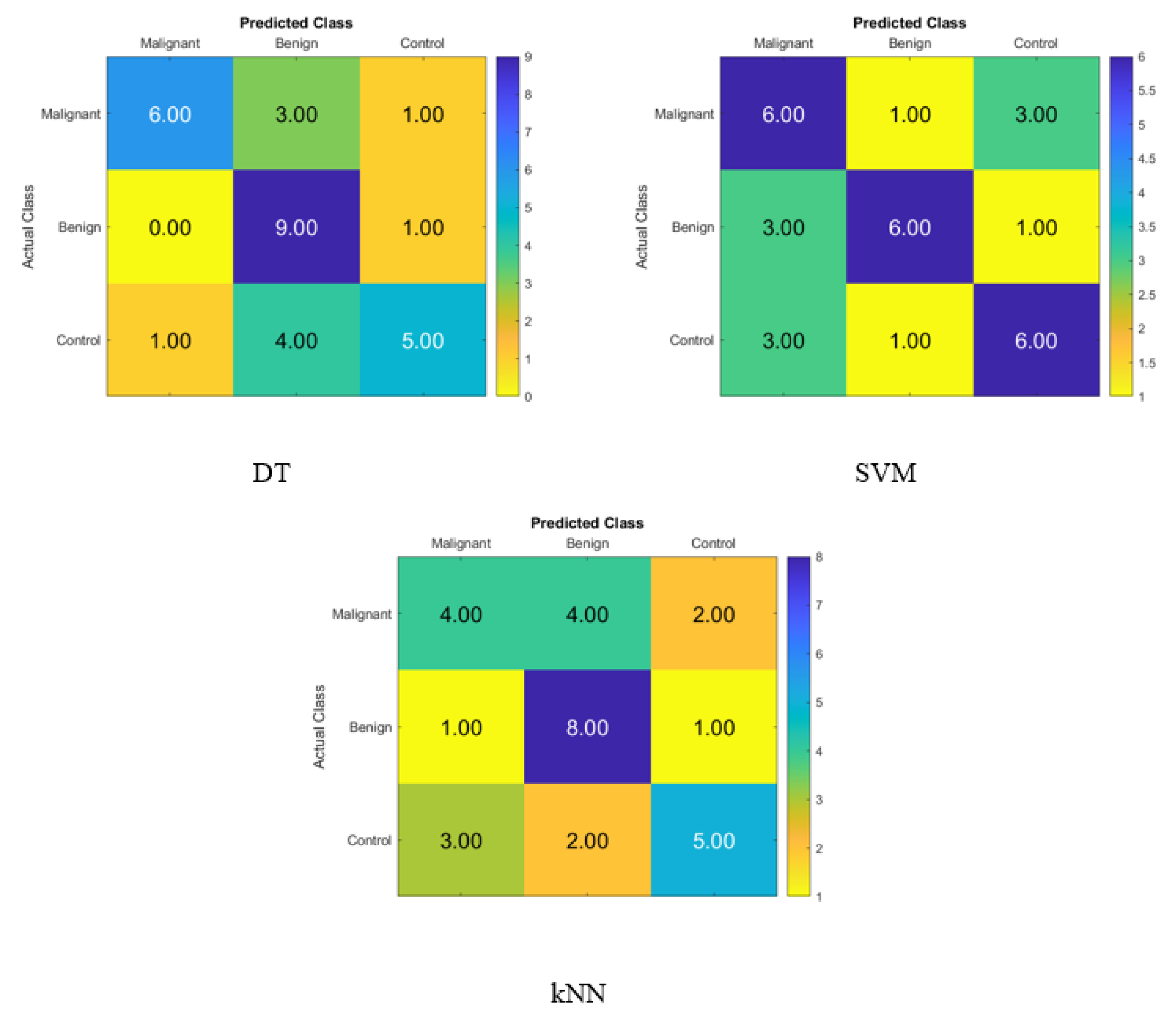
The confusion matrix for identifying normal participants, benign patients, and malignant patients based on the salivary levels of P, T, C, and HCG is depicted in Figure 5, and it was created with statistical features and the KNN, SVM, and DT classifiers in that order. On the diagonal, the right recognition is seen, whereas the off-diagonal areas reflect the incorrect substitutions.

Figure 5.
Confusion matrices for the DT, SVM, and KNN classifiers to demonstrate the saliva hormones performance from the normal subjects, benign patients, and malignant patients.
Figure 5 displays the accuracy rate of the DT, SVM, and KNN classifiers when using the hormone levels in saliva. When compared to the SVM accuracy of 60% and the KNN accuracy of 56.7%, the DT’s accuracy was higher at 66.7%. Hence, the DT correctly identified six malignant patients, nine benign patients, and five control patients. Hence, using the DT, four of the malignant patients were incorrectly classified as one benign patient and one control subject, one benign patient was incorrectly classified as a control subject, and five control subjects were incorrectly classified as one malignant patient and four benign patients.
Table 6 shows the effectiveness of the saliva hormones in normal subjects, benign patients, and malignant patients demonstrated through the use of performance assessment criteria such as precision, sensitivity, specificity, accuracy, and F1-score for the DT, SVM, and KNN classifiers using the FA dimensionality reduction technique.
Table 6.
Performance evaluation, including precision, sensitivity, specificity, accuracy, and F1-score, for the DT, SVM, and KNN classifiers using FA dimensionality reduction technique to show the saliva hormones performance from normal subjects, benign patients, and malignant patients.
Figure 6 depicts the confusion matrix for identifying normal people, benign patients, and malignant patients based on the salivary levels of P, T, C, and HCG using statistical features and FA dimensionality reduction techniques on the KNN, SVM, and DT classifiers, respectively. On the diagonal, the proper recognition is noted, whereas the off-diagonal represents substitution errors.
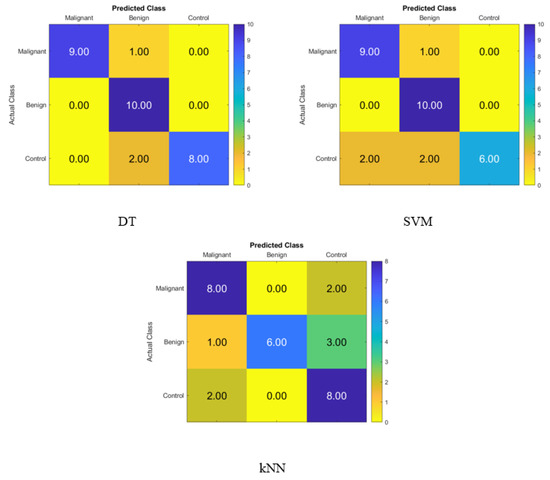
Figure 6.
Confusion matrices for the DT, SVM, and KNN classifiers using FA dimensionality reduction technique to demonstrate the saliva hormones performance from the normal subjects, benign patients, and malignant patients.
Figure 6 depicts the percentage of data that were properly identified by the DT, SVM, and KNN classifiers using FA when the salivary level hormones were used as the variable of interest. The accuracy of the DT was 90%, while that of the SVM was 83.3%, and that of the KNN was 73.3%. Because of this, the DT was shown to be successful in correctly identifying 9 patients with cancer, 10 people with benign conditions, and 8 control patients. Therefore, one malignant patient was incorrectly classified as benign, and two control subjects were incorrectly classified as benign patients.
Table 7 shows the effectiveness of the saliva hormones in normal subjects, benign patients, and malignant patients demonstrated through the use of performance assessment criteria such as precision, sensitivity, specificity, accuracy, and F1-score for the DT, SVM, and KNN classifiers using the t-SNE dimensionality reduction technique.
Table 7.
Performance evaluation, including precision, sensitivity, specificity, accuracy, and F1-score, for the DT, SVM, and KNN classifiers using t-SNE dimensionality reduction technique to show the saliva hormones performance from normal subjects, benign patients, and malignant patients.
Figure 7 shows the confusion matrix for identifying normal subjects, benign patients, and malignant patients from the salivary levels of P, T, C, and HCG using statistical features after using the t-SNE dimensionality reduction techniques and KNN, SVM, and DT classifiers, respectively. The correct recognition is seen on the diagonal, while the substitution errors are seen off of the diagonal. Figure 7 depicts the percentage of the data that was properly identified by the DT, SVM, and KNN classifiers using t-SNE when the salivary level hormones were used as the variable of interest. The accuracy of the DT was 93.3%, while that of the SVM was 80%, and that of the KNN was 76.67%. Because of this, the DT was successful in correctly identifying 9 patients with cancer, 9 people with benign conditions, and 10 control patients. Thus, one malignant patient was incorrectly classified as benign, and one of the benign patients was incorrectly classified as a malignant patient.
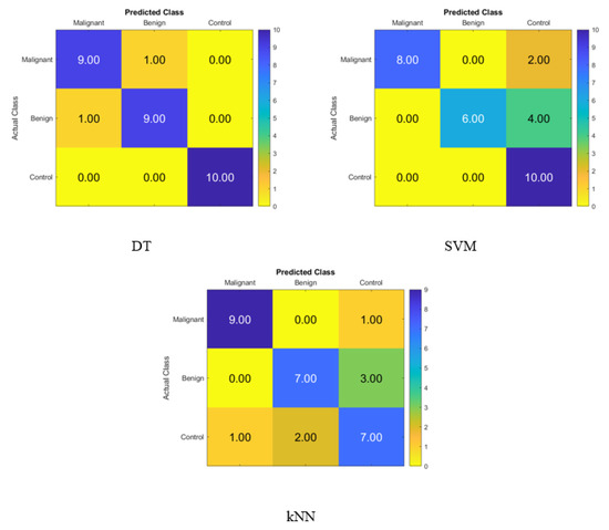
Figure 7.
Confusion matrices for the DT, SVM, and KNN classifiers using t-SNE dimensionality reduction technique to demonstrate the saliva hormones performance from the normal subjects, benign patients, and malignant patients.
5. Discussion
This is the first study that has proven that dimensionality reduction approaches using FA and t-SNE may be used to identify between mild and severe subjects of breast cancer, as well as control women. Even though blood and saliva are not yet widely used as a source of samples for hormone analysis, they are a great research tool that provide a non-invasive and stress-free alternative to plasma and serum. This makes using them an appealing option. These samples have been demonstrated to be trustworthy and, in some situations, superior to other body fluids by displaying a very close association with the free testosterone levels in serum [45]. This has led to their recognition as extremely useful diagnostic tools. Saliva, on the other hand, has several benefits over blood as a sampling medium, including the fact that it may be easily collected by the participants themselves at regular intervals and that it does not require any specialized equipment for collection or storage [46,47]. Hormones such as testosterone serum levels have a low level of reliability in the low ranges that are observed in normal women [48], and their levels can vary greatly depending on genetic, metabolic, and endocrine effects [49]. The concept that the measurements of free or bio-available testosterone are able to more precisely predict androgenic effects than total testosterone levels has recently gained widespread acceptance. In order to ensure the reliability of our research, the 10 generated features corresponded to a total of 10 characteristics for each of the hormones that were analyzed. We made an effort to use all of the possible independent variable statistical features in order to obtain a broad and comprehensive perspective from the blood and saliva in order to classify the severity of BC into normal subjects, benign patients, and malignant cases. This was due to the co-linearity that may exist within this set of derived features, as well as the redundancy that arises from the utilization of the mean and the summation. On the other hand, the discovery that two or more independent variables were correlated leads one to infer that the shifts in one variable are related to changes in another variable. This can happen when two or more variables are found to be correlated. Because of these modifications, we were able to increase the size of the feature set, which was beneficial, given that we wanted to apply methods that reduced the dimensionality of the data. Because of this, the accuracy of the classifiers for the salivary bio-markers varied, which is why the results improved, especially with the DT, with an increase in classification accuracy from 66.67% to 93.3% and 90% when using t-SNE and FA, respectively. The accuracy for the blood biomarkers also improved in the results, particularly with the DT, which saw a boosted classification accuracy from 60% to 80% and 93.3% when utilizing FA and t-SNE, respectively, as statistical tools.
6. Conclusions
BC has claimed the lives of an uncountable number of men and women all over the world. This study applied data mining techniques to the levels of P, T, C, and HCG in the blood and saliva of 60 women with histologically confirmed breast cancer and 20 age-matched control women. A novel approach to the early detection of breast cancer has been proposed. The severity of the BC was categorized into normal, benign, and malignant cases using the proposed technique, which uses blood and saliva as its primary diagnostic tools. The DT, SVM, and KNN models were examined after collecting ten statistical features in order to determine the severity of the BC. These classification techniques were used to identify the severity of the BC. In addition, dimensionality reduction strategies utilizing FA and t-SNE have been computed in order to obtain the most accurate hyper-parameters. Within the framework of the suggested method, the model has been checked for accuracy by utilizing the k-fold cross-validation method. It has been implemented with metrics for determining how effective a model is. The classification accuracy increased from 66.67% to 93.3% and 90%, respectively, using t-SNE and FA for the salivary biomarkers, thanks to dimensionality reduction techniques. The blood biomarker results were further improved by dimensionality reduction methodologies, in particular for the DT, using FA and t-SNE boosting classification accuracy to go from 60% to 80% and 93.3%, respectively. Indeed, dimensionality reduction strategies for blood biomarkers improved the results, particularly for the DT. These tactics increased the classification accuracy from 60% to 80% and 93.33%, respectively, when t-SNE and FA were utilized. These findings suggest t-SNE as a potentially valuable dimension reduction technique that could assist in the identification of patients with different BC severity levels. Nonetheless, the Wisconsin University database has been used by multiple research projects to detect BC. For BC prediction, for example, Rashmi et al. utilized a naive Bayes classifier and yielded an 85% accuracy [19]. In addition, using BC datasets gathered at Leiden University Medical Center, classifiers such as the decision tree algorithm achieved 70% accuracy in their predictions [21]. This is because t-SNE consistently enhances the discrimination between benign and malignant tumours, as well as identifies healthy participants, thereby demonstrating promise as a potential contributor to the advancement of breast cancer screening techniques. In future works, blood tests are going to be integrated with the help of tumor-associated circulating tumor cells, also known as TACTs. This will make it feasible to detect breast cancer at an earlier stage, particularly in people who are at high risk for developing the disease. In addition, the datasets could be expanded, and the applicability of the approach that can be recommended to additional datasets might be investigated.
Author Contributions
Methodology, N.K.A.-Q.; Resources, S.H.B.M.A.; Data curation, I.K.M.; Writing—original draft, N.K.A.-Q.; Writing—review & editing, N.K.A.-Q.; Visualization, H.K.A.-Q.; Supervision, S.A.A. All authors have read and agreed to the published version of the manuscript.
Funding
This research received no external funding.
Institutional Review Board Statement
Not applicable.
Informed Consent Statement
Not applicable.
Data Availability Statement
The data presented in this study are available on request from the corresponding author. The data are not publicly available due to privacy restrictions.
Conflicts of Interest
The authors declare no conflict of interest.
References
- Sung, H.; Ferlay, J.; Siegel, R.L.; Laversanne, M.; Soerjomataram, I.; Jemal, A.; Bray, F. Global cancer statistics 2020: GLOBOCAN estimates of incidence and mortality worldwide for 36 cancers in 185 countries. CA Cancer J. Clin. 2021, 71, 209–249. [Google Scholar] [CrossRef] [PubMed]
- Vamvakas, A.; Tsivaka, D.; Logothetis, A.; Vassiou, K.; Tsougos, I. Breast Cancer Classification on Multiparametric MRI–Increased Performance of Boosting Ensemble Methods. Technol. Cancer Res. Treat. 2022, 21, 15330338221087828. [Google Scholar] [CrossRef] [PubMed]
- Sheth, D.; Giger, M.L. Artificial intelligence in the interpretation of breast cancer on MRI. J. Magn. Reson. Imaging 2020, 51, 1310–1324. [Google Scholar] [CrossRef] [PubMed]
- Thi, T.P. Cartesian Genetic Programming: Some New Detections. In Advances in Information and Communication, Proceedings of the 2022 Future of Information and Communication Conference (FICC), San Francisco, CA, USA, 3–4 March 2022; Springer: Berlin/Heidelberg, Germany, 2022; Volume 2, pp. 294–313. [Google Scholar]
- Haq, A.U.; Li, J.P.; Saboor, A.; Khan, J.; Wali, S.; Ahmad, S.; Ali, A.; Khan, G.A.; Zhou, W. Detection of breast cancer through clinical data using supervised and unsupervised feature selection techniques. IEEE Access 2021, 9, 22090–22105. [Google Scholar] [CrossRef]
- Hassan, N.M.; Hamad, S.; Mahar, K. Mammogram breast cancer CAD systems for mass detection and classification: A review. Multimed. Tools Appl. 2022, 81, 20043–20075. [Google Scholar] [CrossRef]
- Kusy, M.; Kowalski, P.A. Architecture reduction of a probabilistic neural network by merging k-means and k-nearest neighbour algorithms. Appl. Soft Comput. 2022, 128, 109387. [Google Scholar] [CrossRef]
- Dewangan, K.K.; Dewangan, D.K.; Sahu, S.P.; Janghel, R. Breast cancer diagnosis in an early stage using novel deep learning with hybrid optimization technique. Multimed. Tools Appl. 2022, 81, 13935–13960. [Google Scholar] [CrossRef]
- Freeman, K.; Geppert, J.; Stinton, C.; Todkill, D.; Johnson, S.; Clarke, A.; Taylor-Phillips, S. Use of artificial intelligence for image analysis in breast cancer screening programmes: Systematic review of test accuracy. BMJ 2021, 374, 1872. [Google Scholar] [CrossRef]
- Mahoro, E.; Akhloufi, M.A. Applying Deep Learning for Breast Cancer Detection in Radiology. Curr. Oncol. 2022, 29, 8767–8793. [Google Scholar] [CrossRef]
- Jafari, Z.; Karami, E. Breast Cancer Detection in Mammography Images: A CNN-Based Approach with Feature Selection. Information 2023, 14, 410. [Google Scholar] [CrossRef]
- Taylor, C.R.; Monga, N.; Johnson, C.; Hawley, J.R.; Patel, M. Artificial Intelligence Applications in Breast Imaging: Current Status and Future Directions. Diagnostics 2023, 13, 2041. [Google Scholar] [CrossRef]
- Basurto-Hurtado, J.A.; Cruz-Albarran, I.A.; Toledano-Ayala, M.; Ibarra-Manzano, M.A.; Morales-Hernandez, L.A.; Perez-Ramirez, C.A. Diagnostic strategies for breast cancer detection: From image generation to classification strategies using artificial intelligence algorithms. Cancers 2022, 14, 3442. [Google Scholar] [CrossRef]
- Mohammed, I.K.; Al-Timemy, A.H.; Escudero, J. Two-Stage Classification of Breast Tumor Biomarkers for Iraqi Women. Al-Khwarizmi Eng. J. 2020, 16, 1–10. [Google Scholar]
- Van der Maaten, L.; Hinton, G. Visualizing data using t-SNE. J. Mach. Learn. Res. 2008, 9, 2579–2605. [Google Scholar]
- Ayyagari, S.S.; Jones, R.D.; Weddell, S.J. Detection of microsleep states from the EEG: A comparison of feature reduction methods. Med. Biol. Eng. Comput. 2021, 59, 1643–1657. [Google Scholar] [CrossRef] [PubMed]
- Pareek, J.; Jacob, J. Data compression and visualization using PCA and T-SNE. In Advances in Information Communication Technology and Computing, Proceedings of the AICTC 2019, Bikaner, India, 8–9 November 2019; Springer: Berlin/Heidelberg, Germany, 2021; pp. 327–337. [Google Scholar]
- Wattenberg, M.; Viégas, F.; Johnson, I. How to use t-SNE effectively. Distill 2016, 1, e2. [Google Scholar] [CrossRef]
- Rashmi, G.; Lekha, A.; Bawane, N. Analysis of efficiency of classification and prediction algorithms (Naïve Bayes) for Breast Cancer dataset. In Proceedings of the 2015 International Conference on Emerging Research in Electronics, Computer Science and Technology (ICERECT), Mandya, India, 17–19 December 2015; pp. 108–113. [Google Scholar]
- Pritom, A.I.; Munshi, M.A.R.; Sabab, S.A.; Shihab, S. Predicting breast cancer recurrence using effective classification and feature selection technique. In Proceedings of the 2016 19th International Conference on Computer and Information Technology (ICCIT), Dhaka, Bangladesh, 18–20 December 2016; pp. 310–314. [Google Scholar]
- Guo, J.; Fung, B.C.; Iqbal, F.; Kuppen, P.J.; Tollenaar, R.A.; Mesker, W.E.; Lebrun, J.J. Revealing determinant factors for early breast cancer recurrence by decision tree. Inf. Syst. Front. 2017, 19, 1233–1241. [Google Scholar] [CrossRef]
- Zubair, M.; Wang, S.; Ali, N. Advanced approaches to breast cancer classification and diagnosis. Front. Pharmacol. 2021, 11, 632079. [Google Scholar] [CrossRef]
- Tarighati, E.; Keivan, H.; Mahani, H. A review of prognostic and predictive biomarkers in breast cancer. Clin. Exp. Med. 2022, 23, 1–16. [Google Scholar] [CrossRef]
- Wang, H.; Yoon, S.W. Breast cancer prediction using data mining method. In Proceedings of the IIE Annual Conference, Nashville, TN, USA, 30 May–2 June 2015; Institute of Industrial and Systems Engineers (IISE): Peachtree Corners, GA, USA, 2015; p. 818. [Google Scholar]
- Mining, D. Application of data mining techniques to predict breast cancer. Procedia Comput. Sci. 2019, 163, 11–18. [Google Scholar]
- Cesar, M.O.R.; German, L.B.; Patricia, A.C.P.; Eugenia, A.R.; Clementina, O.M.E.; Jose, C.O.; Alberto, P.M.M.; Enrique, M.P.F.; Margarita, R.V. Method based on data mining techniques for breast cancer recurrence analysis. Adv. Swarm Intell. 2020, 12145, 584. [Google Scholar]
- Wassim, A.; Elarbi, E.; Khadija, R. Application of Machine Learning Approaches in Health Care Sector to The Diagnosis of Breast Cancer. Proc. J. Phys. Conf. Ser. 2022, 2224, 012012. [Google Scholar] [CrossRef]
- Li, J.; Guan, X.; Fan, Z.; Ching, L.M.; Li, Y.; Wang, X.; Cao, W.M.; Liu, D.X. Non-invasive biomarkers for early detection of breast cancer. Cancers 2020, 12, 2767. [Google Scholar] [CrossRef] [PubMed]
- Sun, Y.; Du, W.; Yang, L.L.; Dai, M.; Dou, Z.Y.; Wang, Y.X.; Liu, J.; Zheng, G. Computational methods for recognition of cancer protein markers in saliva. Math. Biosci. Eng. 2020, 17, 2453–2469. [Google Scholar] [CrossRef] [PubMed]
- Assad, D.X.; Mascarenhas, E.C.P.; de Lima, C.L.; de Toledo, I.P.; Chardin, H.; Combes, A.; Acevedo, A.C.; Guerra, E.N.S. Salivary metabolites to detect patients with cancer: A systematic review. Int. J. Clin. Oncol. 2020, 25, 1016–1036. [Google Scholar] [CrossRef] [PubMed]
- Indira, V.; Vasanthakumari, R.; Jegadeeshwaran, R.; Sugumaran, V. Determination of minimum sample size for fault diagnosis of automobile hydraulic brake system using power analysis. Eng. Sci. Technol. Int. J. 2015, 18, 59–69. [Google Scholar] [CrossRef]
- Van Der Maaten, L.; Postma, E.; Van den Herik, J. Dimensionality reduction: A comparative. J. Mach. Learn Res. 2009, 10, 13. [Google Scholar]
- Tăuţan, A.M.; Rossi, A.C.; de Francisco, R.; Ionescu, B. Dimensionality reduction for EEG-based sleep stage detection: Comparison of autoencoders, principal component analysis and factor analysis. Biomed. Eng. Tech. 2021, 66, 125–136. [Google Scholar] [CrossRef]
- Salod, Z.; Singh, Y. Comparison of the performance of machine learning algorithms in breast cancer screening and detection: A protocol. J. Public Health Res. 2019, 8, jphr-2019. [Google Scholar] [CrossRef]
- Vapnik, V. The Nature of Statistical Learning Theory; Springer Science & Business Media: Berlin/Heidelberg, Germany, 1999. [Google Scholar]
- Al-Qazzaz, N.K.; Ali, S.; Ahmad, S.A.; Escudero, J. Classification enhancement for post-stroke dementia using fuzzy neighborhood preserving analysis with QR-decomposition. In Proceedings of the 2017 39th Annual International Conference of the IEEE Engineering in Medicine and Biology Society (EMBC), Jeju, Republic of Korea, 1–15 July 2017; pp. 3174–3177. [Google Scholar]
- Aha, D.W.; Kibler, D.; Albert, M.K. Instance-based learning algorithms. Mach. Learn. 1991, 6, 37–66. [Google Scholar] [CrossRef]
- Hart, P.E.; Stork, D.G.; Duda, R.O. Pattern Classification; Wiley: Hoboken, NJ, USA, 2000. [Google Scholar]
- Kantardzic, M. Data Mining: Concepts, Models, Methods, and Algorithms; John Wiley & Sons: Hoboken, NJ, USA, 2011. [Google Scholar]
- Aldea, R.; Fira, M.; Lazăr, A. Classifications of motor imagery tasks using k-nearest neighbors. In Proceedings of the 12th Symposium on Neural Network Applications in Electrical Engineering (NEUREL), Belgrade, Serbia, 25–27 November 2014; pp. 115–120. [Google Scholar]
- Agarwal, S. Data mining: Data mining concepts and techniques. In Proceedings of the 2013 International Conference on Machine Intelligence and Research Advancement, Katra, India, 21–23 December 2013; pp. 203–207. [Google Scholar]
- Al-Qazzaz, N.K.; Ali, S.H.B.M.; Ahmad, S.A.; Escudero, J. Optimal EEG channel selection for vascular dementia identification using improved binary gravitation search algorithm. In Proceedings of the 2nd International Conference for Innovation in Biomedical Engineering and Life Sciences: ICIBEL 2017 (in Conjunction with APCMBE 2017), Penang, Malaysia, 10–13 December 2017; Springer: Berlin/Heidelberg, Germany, 2017; pp. 125–130. [Google Scholar]
- Al-Qazzaz, N.K.; Ali, S.H.M.; Ahmad, S.A. Differential evolution based channel selection algorithm on EEG signal for early detection of vascular dementia among stroke survivors. In Proceedings of the 2018 IEEE-EMBS Conference on Biomedical Engineering and Sciences (IECBES), Sarawak, Malaysia, 3–6 December 2018; pp. 239–244. [Google Scholar]
- Lehmann, C.; Koenig, T.; Jelic, V.; Prichep, L.; John, R.E.; Wahlund, L.O.; Dodge, Y.; Dierks, T. Application and comparison of classification algorithms for recognition of Alzheimer’s disease in electrical brain activity (EEG). J. Neurosci. Methods 2007, 161, 342–350. [Google Scholar] [CrossRef] [PubMed]
- Dimitrakakis, C.; Zava, D.; Marinopoulos, S.; Tsigginou, A.; Antsaklis, A.; Glaser, R. Low salivary testosterone levels in patients with breast cancer. BMC Cancer 2010, 10, 547. [Google Scholar] [CrossRef] [PubMed]
- Glaser, R.L.; Zava, D.T.; Wurtzbacher, D. Pilot study: Absorption and efficacy of multiple hormones delivered in a single cream applied to the mucous membranes of the labia and vagina. Gynecol. Obstet. Investig. 2008, 66, 111–118. [Google Scholar] [CrossRef] [PubMed]
- Cook, C.J. Rapid noninvasive measurement of hormones in transdermal exudate and saliva. Physiol. Behav. 2002, 75, 169–181. [Google Scholar] [CrossRef] [PubMed]
- Lobo, R.A. Androgens in postmenopausal women: Production, possible role, and replacement options. Obstet. Gynecol. Surv. 2001, 56, 361–376. [Google Scholar] [CrossRef]
- Tchernof, A.; Després, J.P. Sex steroid hormones, sex hormone-binding globulin, and obesity in men and women. Horm. Metab. Res. 2000, 32, 526–536. [Google Scholar] [CrossRef]


Disclaimer/Publisher’s Note: The statements, opinions and data contained in all publications are solely those of the individual author(s) and contributor(s) and not of MDPI and/or the editor(s). MDPI and/or the editor(s) disclaim responsibility for any injury to people or property resulting from any ideas, methods, instructions or products referred to in the content. |
© 2023 by the authors. Licensee MDPI, Basel, Switzerland. This article is an open access article distributed under the terms and conditions of the Creative Commons Attribution (CC BY) license (https://creativecommons.org/licenses/by/4.0/).