Article

Using an Artificial Physarum polycephalum Colony for Threshold Image Segmentation

Hubei Province Engineering Technology Research Center for Construction Quality Testing Equipments, College of Computer and Information Technology, China Three Gorges University, Yichang 443002, China
*
Author to whom correspondence should be addressed.
Appl. Sci. 2023, 13(21), 11976; https://doi.org/10.3390/app132111976
Submission received: 12 August 2023 / Revised: 21 October 2023 / Accepted: 30 October 2023 / Published: 2 November 2023

Abstract

:

Featured Application

Image segmentation can be applied to image recognition and computer vision as the most important preprocess, and theartificial Physarum polycephalum colony algorithm proposed in this article can also be used to solveall kinds of complex problems in image processing.

Abstract

Traditional artificial intelligence algorithms are prone to falling into local optima when solving threshold segmentation problems. Here, a novel artificial Physarum polycephalum colony algorithm is proposed to help us solve the difficult problem. First, the algorithm methodology of an artificial Physarum polycephalum colony algorithm is described to search for the optimal solutions by expansion and contraction of a lot of artificial hyphae. Different artificial Physarum polycephalum can learn from each other and produce more hyphae in expansion. In contraction, the artificial Physarum polycephalum colony can select the best hyphae with high fitness through a quick sort algorithm, but the other hyphae with low fitness will be absorbed and disappear. Second, a fitness function is modeled based on Kapur’s entropy for the proposed artificial Physarum polycephalum colony algorithm to search for optimal threshold segmentation solutions. Third, a series of benchmark experiments are implemented to test the proposed artificial Physarum polycephalum colony algorithm, and some state-of-the-art approaches are employed for comparison. The experimental results verified that the proposed algorithm can obtain better accuracy and convergence speed, and is not easier to fall into the local optimal solution too early.

1. Introduction

Image segmentation is a key step from image processing to image analysis. Among them, threshold segmentation is the most commonly used parallel region technique and also the category with the highest number of applications in image segmentation. Threshold image segmentation employs the image gray-level histogram and one or more thresholds to segment an image [1]. This method compares the gray values between the target and the background on an image and selects appropriate thresholds to implement image segmentation where it judges each pixel belonging to the target region or the background region [2]. Now, the threshold image segmentation method is the most widely used and has become an essential link in image processing, i.e., COVID-19 diagnosis [2], satellite monitoring [3], remote sensing analysis [4], fault diagnosis [5], carotid artery surgery [6], prevention and control of maize diseases [7], CT scan [8], etc. Peak signal-to-noise ratio (PSNR) and feature similarity (FSIM) are often used indexes for performance evaluation of threshold image segmentation.
The selection of a threshold is important for threshold segmentation methods since only accurate threshold selection can ensure the accuracy of threshold image segmentation [9]. Recently, more and more scholars are getting involved in this area and trying to find the optimal threshold. For a given image, the optimal threshold can often be determined by analyzing its histogram. For example, when the histogram clearly shows a bimodal pattern, the midpoint of the two peaks can be selected as the optimal threshold [10]. According to the dimension, the image histogram can be classified into one-dimensional (1-D) histogram, two-dimensional (2-D) histogram, three-dimensional (3-D) histogram [3,11], and so on. Because of the complexity of images and the uncertainty of noise interference, determining the appropriate threshold through histograms is still not an easy task [12].
Due to the difficulty of manually selecting thresholds, many scholars have begun to use artificial intelligence algorithms to help us determine appropriate thresholds and many algorithms are verified to have great potential in the field of threshold image segmentation [6,9]. Among them, swarm intelligence is a hotspot that simulates the behaviors of a swarm of animals in foraging and living. For example, the whale optimization algorithm (WOA) [1], Harris hawks optimization (HHO) [2], artificial neural networks (ANNs) [3,11], deep learning (DL) [4,12], gray wolf optimization (GWO) [5], particle swarm optimization (PSO) [7], differential evolution algorithm (DEA) [9], cuckoo search algorithm (CSA) [10], ant colony optimization (ACO) [13], genetic algorithm (GA) [14], artificial bee colony algorithm (ABC) [15], sparrow search algorithm (SSA) [16], and so on. Recent works verified that swarm intelligence algorithms can obtain good performance and are promising to solve image segmentation problems. However, the heuristic search used by artificial intelligence algorithms also easily to falls into the local optimal solution too early due to the probabilistic [6,9].
Inspired by the intelligent behavior of a natural Physarum polycephalum, which can produce a large number of hyphae to search for food [17,18], a novel artificial Physarum polycephalum colony algorithm (APPCA) is proposed to help us solve the threshold image segmentation. The main contributions of this article are as follows:
  • To overcome the shortcomings of an algorithm search, an APPCA is designed, which can search for the optimal solutions by the expansion and contraction of a lot of artificial hyphae. Different Physarum polycephalum hyphae can learn from each other and produce more hyphae in expansion to enhance the global search capability. In contraction, the artificial Physarum polycephalum colony (APPC) can select the best hyphae with the highest fitness values through a quick sort algorithm to improve the convergence performance. Different from traditional artificial intelligence algorithms, the population sizes of APPCA in expansion and contraction are different, and the proposed algorithm uses a variable population size to search for optimal segmented images.
  • To explore the average information content of different pixels in image segmentation, a fitness function is modeled based on Kapur’s entropy for the proposed artificial Physarum polycephalum colony algorithm to search for the optimal threshold segmentation solutions. The fitness function can help the APPCA solve the image segmentation problem with high accuracy and short computational time.
  • To test the proposed artificial Physarum polycephalum colony algorithm, a series of benchmark experiments are implemented, and some state-of-the-art approaches are compared. The experimental results verified the effectiveness of the proposed APPCA. The APPCA can obtain better accuracy and convergence speed, and is not easier to fall into the local optimal solution too early compared with traditional artificial intelligence algorithms.
The remainder of this paper is organized as follows. Section 2 reviews the related work. Section 3 introduces the threshold image segmentation based on APPCA. Section 4 analyzes the fitness function and the convergence of the APPCA. Section 5 implements benchmark tests for the performance of the APPCA and compares some state-of-the-art algorithms. Finally, this paper is concluded in Section 6.

2. Related Work

Threshold image segmentation is a widely used segmentation technology, where an image is regarded as a combination of two types of areas, i.e., target areas and background areas with different grayscale levels [19]. Taking advantage of the difference between the target areas and the background areas in the grayscale characteristics, threshold image segmentation can generate a corresponding binary image by extracting the target areas [20]. In threshold image segmentation, a reasonable threshold is essential to determine whether each pixel in the image should belong to the target areas or the background areas. Hence, the key in threshold image segmentation is to search for the appropriate threshold accurately and quickly.
To find optimal thresholds in image segmentation, recent researchers selected different methods as follows.
First, the threshold in most cases can be determined by the separation between gray peaks in a histogram of the original image. The gray level of an original image usually presents normal distribution in target and background areas, so the image gray histogram tends to have two single peaks corresponding to the target and background areas, respectively [21]. The adjacent pixels between the target or background areas are correlated in the gray level, but the pixels at the junction of the target and background areas are different in the gray level [22]. In this case, the bottom of the gray level valley between the two peaks can be selected as a threshold.
Second, Ostu proposed the inter-class variance threshold segmentation method in 1979, which divides the image into foreground and background parts based on its grayscale distribution [1,7]. The segmentation values of the foreground and background are calculated using the inter-class variance method to obtain the threshold, so the foreground is the part we segmented. Ref. [23] described an Otsu multi-threshold image segmentation based on an improved particle swarm algorithm.
Third, multi-threshold segmentation is based on multiple valleys appearing in the grayscale histogram as segmentation points, using multiple thresholds to segment multiple peaks [2]. Therefore, there are as many target regions as there are peaks. Ref. [5] illustrated a fault diagnosis algorithm of gearboxes based on GWO-SCE adaptive multi-threshold segmentation and subdomain adaptation. The gray value of pixels may change by noise and produce an imbalance in the histogram of an original image, so the bottom of a histogram may be filled to generate new peaks [7]. Hence, the bottom of the gray level valley between the two peaks can be segmented by multi-threshold [9,10,13].
Fourth, multi-level segmentation can segment an image into multiple sets of segmentation results with different levels of detail at different scales and can determine the relative size between the targets and background [24]. Ref. [25] employed a multi-level image threshold segmentation using an improved Bloch quantum artificial bee colony algorithm. In many original images, there are a lot of small targets or large targets, so it is not easy to determine the valley bottom in the histogram. Traditional single-level image segmentation results in severe loss of final feature hotspots and resolution, leading to a lack of detail characterization ability in segmentation results [26,27]. Multi-level threshold segmentation forms a multi-level network structure representation of the same image at different scales [28,29].
Fifth, dynamic threshold segmentation does not require artificially setting thresholds, but rather segments based on the features present in the image [20]. Dynamic threshold segmentation generally compares the original image with the processed image to generate a difference image and then calculates the bright or dark regions in the difference image. The brightness of the target and background may vary with the illumination, such as maize diseases [7] and cucumber seedlings [14]. Dynamic threshold segmentation has the characteristics of strong anti-interference and stability and is not sensitive to changes in lighting. Ref. [30] explored an unsupervised segmentation method based on dynamic threshold neural P systems for color images.
Sixth, the entropy threshold can describe the degree to which certain material system states may occur, so some researchers employed entropy to depict the texture feature on an original image and select an entropy threshold for image segmentation [31]. Ref. [13] introduced a multi-threshold image segmentation for melanoma based on Kapur’s entropy using enhanced ant colony optimization. Kapur’s entropy focused on evaluating the compactness of all defined clusters since the intensity follows the cluster’s distribution. An entropy threshold with the maximization of Kapur’s entropy can search for the clusters around the cluster’s centroid and central pixels without outliers.
Therefore, threshold selection and image segmentation involve too many factors, making such heavy tasks and calculations extremely challenging for the human brain [32,33]. Nowadays, with the help of artificial intelligence technology, it is entirely possible to entrust such complex tasks to computers, and they can be performed faster and more accurately than the human brain [6]. Artificial intelligence is the study of the laws of human intelligence activities, the construction of artificial systems with a certain level of intelligence, and the study of how to enable computers to perform tasks that previously required human intelligence, that is, the study of how to apply the basic theories, methods, and techniques of computer software and hardware to simulate certain intelligent behaviors of humans. For example, fuzzy set theory can be applied to a wide range of fields with incomplete or imprecise image segmentation, such as the fuzzy c-means method [34,35,36]. Wavelet transform is a local transformation of space and frequency, which can effectively extract information from the original images [36,37]. The application of artificial intelligence has made contemporary people no longer consider threshold selection and image segmentation as complex tasks that must be completed by human manual operation.`
Swarm intelligence is an important kind of artificial intelligence, and further, it is a subdomain of combinatorial optimization in intelligent computing. Its algorithm is affected by the natural selection mechanism of “survival of the fittest” in the process of biological evolution and the transmission law of genetic information. Through program iteration simulation of this process, the problem to be solved is regarded as the environment, and the optimal solution is found through natural evolution in the population composed of some possible solutions. In the process of searching for the optimal threshold, the fitness function plays an important role in swarm intelligence. If the fitness is high, the swarm will take the pixel value as a threshold. Hence, the higher the fitness is, the greater the swarm finds the threshold to segment the target from the background. Common swarm intelligence algorithms include the whale optimization algorithm [1,29], Harris hawks optimization [2], artificial neural networks [3,11,30], deep learning [4,12,21,38], gray wolf optimization [5,39], particle swarm optimization [7,23,40], differential evolution algorithm [9], cuckoo search algorithm [10], ant colony optimization [13,33], genetic algorithm [14,40], artificial bee colony algorithm [15,25], sparrow search algorithm [16], moth swarm algorithm (MSA) [24], emperor penguin optimization (EPO) [26], marine predators algorithm (MPA) [27], salp swarm algorithm (SSA) [27], firefly algorithm (FA) [28], Aptenodytes Forsteri optimization algorithm (AFOA) [32], artificial fish swarm algorithm (AFSA) [36], artificial plant community (APC) [41,42], krill swarm (KS) [43], immune system (IS) [44], naked mole-rat algorithm (NMRA) [45], attention mechanism [46], and so on.
Although swarm intelligence algorithms have been proven effective, they have also been complained of being prone to premature local optima. The Physarum polycephalum in nature can stretch out tens of thousands of filamentous hyphae to search for surrounding food [17,18,47]. This inspires us as to whether the swarm intelligence of Physarum polycephalum can be utilized to provide us with a more efficient algorithm for solving image segmentation problems.

3. Methodology

Here, the mathematical model of threshold image segmentation is built as a multi-objective function with an entropy threshold. The symbol definition is provided in Section 3.1, the artificial Physarum polycephalum colony is designed in Section 3.2, the multi-objective fitness function is built in Section 3.3, the performance measurement is provided in Section 3.4, and the algorithm flow is illustrated in Section 3.5.

3.1. Symbol Definitions

In our proposed model, each Physarum polycephalum hyphae is a feasible solution and is evaluated by a fitness function, which determines the searching and learning of hyphae and the optimization process of threshold image segmentation. The proposed model employs Kapur’s entropy [13] to calculate the fitness function and variance for Physarum polycephalum colony to improve the segmentation performance. The symbol definition is shown in Table 1.
In threshold image segmentation, it processes an original image O into a segmented image A with a grayscale level L. Both images have the same image size H in the horizontal direction and the same image size V in the vertical direction. Hence, the total number of pixels on the original image is N = HV. The threshold segmentation can be implemented by an artificial Physarum polycephalum colony with a population size of S, and instructed by a fitness function fit based on Kapur’s entropy of K. The segmentation of image A can be compared with the benchmark image B, where a pixel a i j has a pair of coordinates (i, j) on the gray image A and a pixel b i j has a pair of coordinates (i, j) on the benchmark image B.

3.2. Artificial Physarum polycephalum Colony

In this subsection, to overcome the shortcomings of algorithm search, a novel artificial Physarum polycephalum colony is designed on the basis of natural Physarum in the literature [17,18,47]. 
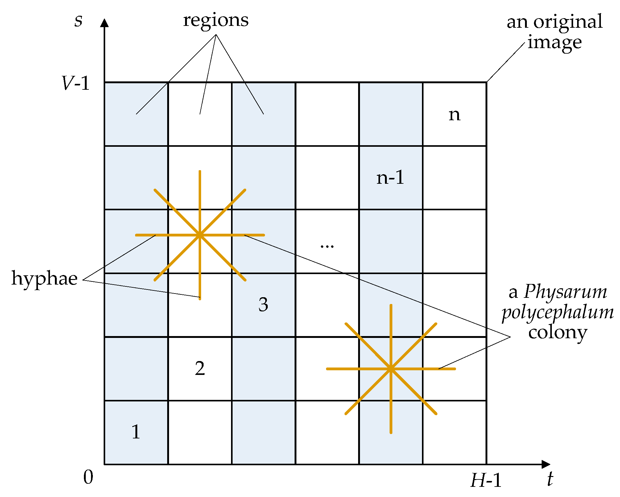
Figure 1 shows an artificial Physarum polycephalum colony on a 2-D segmentation image. In our artificial Physarum polycephalum colony algorithm, there are three main components, i.e., an original image, an artificial Physarum polycephalum colony, and a fitness function.
First, the original image in Figure 1 is not only the living area of an artificial Physarum polycephalum colony but also the solution space of the threshold image segmentation or other complex problems. In an original image, there are a lot of pixels with different gray levels. An artificial Physarum polycephalum colony can search for feasible solutions on an original image or solution space. Each feasible solution is a segmentation model of the original image. The artificial Physarum polycephalum colony should search for feasible solutions as the food sources for its living and the feasible solutions are randomly distributed in the solution space. The food sources can be absorbed by the artificial Physarum polycephalum colony and changed into nutrients flowing in its body.
Second, several Physarum polycephalum constitute an artificial Physarum polycephalum colony in Figure 1, where an artificial Physarum polycephalum employs many filiform hyphae to randomly search for feasible solutions. The artificial Physarum polycephalum colony algorithm counts the number of hyphae as the population size S. The artificial Physarum polycephalum colony employs three learning mechanisms, i.e., self-learning, social learning, and free learning. Hence, different hyphae can learn from each other and many hyphae can cross to share the environmental information. The artificial Physarum polycephalum finding the food sources and obtaining more nutrients will survive; otherwise, it will be absorbed and disappear. The leaning mechanism and absorbing behavior can effectively simulate the swarm behavior of a real Physarum polycephalum colony.
Third, the artificial Physarum polycephalum colony utilizes a fitness function to evaluate its living state, which is not shown in Figure 1. The threshold t and region threshold s segment the original image into several parts, and the fitness depends on the nutrients from the food sources. The artificial Physarum polycephalum colony does not know the positions of the feasible solutions from the beginning, but it can judge the feasible solution by a fitness function. If an artificial Physarum polycephalum or a hyphae finds a solution, it will obtain a high fitness value. The fitness function can be designed according to the problems to be solved, such as threshold image segmentation. Different artificial Physarum polycephalum can cross and learn the nutrient information to share the fitness information.
Based on the three basic components, the artificial Physarum polycephalum colony algorithm uses two main operations to search for the optimal solutions, i.e., expansion and contraction.
In the expansion operation, the artificial Physarum polycephalum colony employs three learning mechanisms to produce more hyphae, i.e., self-learning, social-learning, and free-learning. At the initialization, the artificial Physarum polycephalum colony produces a population size S of filiform hyphae, where each filiform hyphae is a randomly generated feasible solution. In expansion, the filiform hyphae with a population size of S remain unchanged by self-learning, and all these artificial Physarum polycephalum hyphae can learn from each other’s experience to produce a new generation of hyphae with a population size of S by social-learning. At the same time, the artificial Physarum polycephalum colony will search the whole solution space by free learning to randomly generate several new hyphae completely unrelated to existing hyphae. Now, the population size of hyphae in expansion operation is greater than twice the original state 2S.
In contraction operation, the artificial Physarum polycephalum colony calculates the fitness of all hyphae according to the fitness function and selects the top S best hyphae. Other hyphae with low fitness will be absorbed and disappear. Now, the population size of hyphae in contraction operation restores to the initial value S. The contraction operations can help the artificial Physarum polycephalum colony converge to the optimal solution and eliminate hyphae with low fitness. After multiple expansion and contraction iterations and fitness comparisons, the artificial Physarum polycephalum colony can find the optimal solution to the threshold image segmentation.

3.3. A Fitness Function for Entropy Threshold

This subsection provides the fitness function for the artificial Physarum polycephalum colony to implement threshold image segmentation. To explore the average information content of different pixels in image segmentation, the fitness of the proposed threshold image segmentation is based on the maximum entropy model proposed by Kapur [13,40] and maximizes the total entropy of the segmented target and background. The Kapur’s entropy can help us obtain the largest amount of segmentation information on an original image.
In different threshold models, the 1-D segmentation method is the fastest in segmentation speed since it does not consider the gray values of different pixels on an original image. The 3-D segmentation is the lowest in segmentation speed since it considers 3-D gray information. The 2-D segmentation method is between 1-D and 3-D in image segmentation speed since it considers the gray information of each pixel and its neighborhood but not the 3-D gray information. Here, 2-D segmentation is employed since it can obtain balanced performance, as shown in Figure 1. A set of thresholds t = { t 1 , t 2 , t 3 , , t n } segments the target and background into several regions, and the other regions are mainly image noise.
The fitness function should instruct the artificial Physarum polycephalum colony to be efficient and accurate in searching for the best threshold ( t 1 , t 2 , t 3 , , t n ) to obtain the best segmentation quality. A good fitness function should make full use of the gray information of the original image and suppress the noise from target and background areas.
Here, the Kapur’s entropy K t 1 , t 2 , t 3 , , t n can be calculated for the set of thresholds ( t 1 , t 2 , t 3 , , t n ) as follows [13,40]:
K t 1 , t 2 , t 3 , , t n = i = 0 n K i ,
where K t 1 , t 2 , t 3 , , t n indicates Kapur’s entropy in all areas. Hence, Kapur’s entropy in each area can be computed as
K 0 = i = 0 t 1 1 p i w 0 ln p i w 0 ; w 0 = i = 0 t 1 1 p i
K 1 = i = t 1 t 2 1 p i w 1 ln p i w 1 ; w 1 = i = t 1 t 2 1 p i
K n = i = t n L 1 p i w n ln p i w n ; w n = i = t n L 1 p i ,
where the parameters w0, w1, …, wn indicate the possibility for each segmentation cluster, and pi indicates the possibility of the occurrence of pixels with a gray value i. Now, Kapur’s entropy can be obtained for each cluster and instruct the artificial Physarum polycephalum colony to evaluate the characteristics of clusters. There is
f i t = a r g m a x { K t 1 , t 2 , t 3 , , t n } .
The combination maximization function fit is the optimal threshold group. The artificial Physarum polycephalum colony uses the fitness function to select the optimal solution. The higher the fitness function, the better the quality is achieved.

3.4. Performance Measurement

This subsection describes the evaluation indicators for the performance measurement of threshold image segmentation. These indicators can measure the segmentation performance from different aspects based on the original image, where the original image is a reference and the segmentation models from the same original image are subjected to the image noise. In the benchmark tests of Section 5, the indicators can help us compare the performance difference between the proposed APPC algorithm and the traditional artificial intelligence ones.
First, the mean squared error (MSE) is a popular index to measure the difference between two images by computing the average sum of the squares between two images. The MSE can evaluate the total difference of all pixels on two whole images, where a lower MSE value means less difference between two images. The MSE can be written as follows:
M S E = 1 H V i = 1 H j = 1 V ( a i j b i j ) 2 ,
where H represents the image size in the horizontal direction, V represents the image size in the vertical direction, aij is a pixel on the segmented image A with a pair of coordinates (i, j), and bij is a pixel on the benchmark image B with a pair of coordinates (i, j). The drawback of MSE is that the value often has the same weight in different grayscale. For example, a high MSE can be obtained from a noisy background on a well-recognizable image.
Second, the peak signal-to-noise ratio (PSNR) is an important indicator of the quality of image segmentation. It calculates the ratio of the effective signal to the noise signal on an image, that is, the ratio of the segmented image to the benchmark image. According to the mean square deviation in Equation (6), the PSNR can be defined for two images with the same size:
P S N R = 10 × l o g ( L 2 M S E )
where MSE is the mean squared error in Equation (6), and L is the grayscale level of the image. A high PSNR often means high quality, and a low PSNR often means low quality. A high PSNR also indicates good image recognition.
Third, the correlation coefficient (CorCoe) is also a popular indicator to measure the linear correlation between two images. The CorCoe can compare the intensity difference of each pixel between two images and the average intensity difference between two whole images. The CorCoe can be calculated as follows:
C o r C o e = i H j V ( A i j A ¯ ) ( B i j B ¯ ) i H j V ( A i j A ¯ ) 2 i H j V ( B i j B ¯ ) 2
where A i j and B i j indicate the intensity value on each pixel with a pair of coordinates (i, j) for two images A and B, respectively. A ¯ and B ¯ indicate the arithmetic mean of intensity value for two images A and B, respectively. H represents the image size in the horizontal direction, and V represents the image size in the vertical direction. The CorCoe metric often takes values in [−1, 1], where 1 represents the highest match between two images, but −1 represents the lowest match between two images.
Fourth, Jaccard’s index (Jaccard), also called Intersection-Over-Union, IoU, is another popular indicator to measure the segmentation quality. The Jaccard metric calculates the size of the intersection divided by the union size of each set of pixels to measure the similarity between finite sets of pixels. The calculation equation can be obtained as follows:
J a c c a r d = | A B | | A B | = | A B | A + B | A B |
where A is the segmented image with additive noise and B is the benchmark image. The numerator | A B | calculates the overlap area of images A and B, and the denominator | A B | describes the fusion area of images A and B. Jaccard index ranges from 0 to 1, where a value of 1 indicates a perfect overlap or the greatest similarity, but a value of 0 indicates no spatial overlap or an absolute mismatch.
Fifth, the Sørensen Dice coefficient (Dice) is similar to Jaccard’s coefficient but is the double overlap region divided by the total number of pixels in two images. The Dice and Jaccard are positively correlated and are easy to reach a consensus assessment. For example, they both may determine model A is better than model B in segmentation performance, or vice versa. The calculation equation is as follows:
D i c e = 2 | A B | A + B = 2 | A B | A B + | A B |
where A is the segmented image with additive noise and B is the benchmark image. The numerator | A B | calculates the overlap area of images A and B, and the denominator | A B | describes the fusion area of images A and B. Dice coefficient also ranges from 0 to 1, where a value of 1 indicates a perfect overlap or the greatest similarity, but a value of 0 indicates no spatial overlap or an absolute mismatch.
Sixth, the Structural Similarity Index (SSIM) calculates a multiplicative combination of three image components, i.e., brightness, contrast, and texture. The SSIM can describe the scene structure information on an image.
For a gray image A, the average gray level μ A can be calculated to estimate the brightness, so the brightness can be written as follows:
μ A = 1 H V i = 1 H j = 1 V a i j ,
where H represents the image size in the horizontal direction, V represents the image size in the vertical direction, and aij is a pixel on the segmented image A with a pair of coordinates (i, j).
The measurement system removes the average grayscale value μ A from the image. For a digital image A, standard deviation σ A can be used as the contrast estimation value.
σ A = 1 H V 1 i = 1 H j = 1 V ( x i j μ A ) 2
According to the brightness μ A in Equation (11) and the contrast σ A in Equation (12), the texture can be expressed as their function. Therefore, the SSIM can be calculated as follows:
S S I M = ( 2 μ A μ B + C 1 ) ( 2 σ A σ B + C 2 ) ( μ A 2 + μ B 2 + C 1 ) ( σ A 2 + σ B 2 + C 2 )
where the average gray level μ A and μ B estimates the brightness, and the standard deviation σ A and σ B evaluates the contrast. The constant C 1 is used to avoid instability of the evaluation system when the brightness approaches 0, often C 1 = ( K 1 L ) 2 . L is the grayscale level of the image, i.e., L = 255 for 8-bit grayscale images. K 1 is a positive constant far less than 1. The constant C 2 is used to avoid instability of the evaluation system when the contrast approaches 0, often C 2 = ( K 2 L ) 2 . L is the grayscale level of the image, and K 2 is a positive constant far less than 1.
In the experimental results of Section 5, the performance measurement indicators above are employed for objective evaluation and algorithm comparison, which can objectively verify the proposed APPC algorithm and compare the segmentation performance.

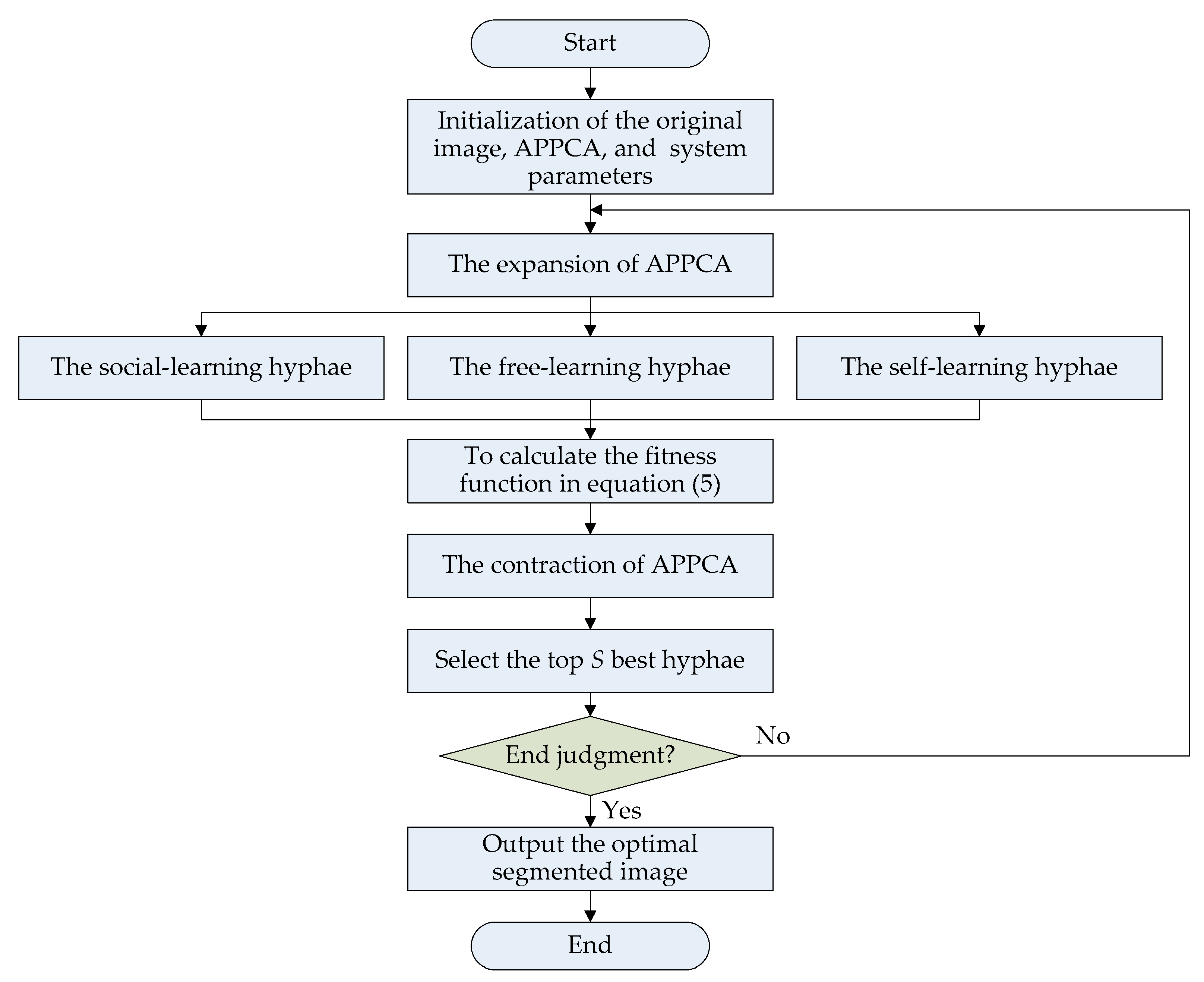
3.5. Algorithm Flow of APPCA

This subsection provides the algorithm flow of APPCA. To solve the threshold image segmentation problem, all Physarum polycephalum will continuously search for the optimal solutions by iterative computation according to the algorithm flow, as shown in Figure 2. The whole algorithm flow includes four main stages, namely initialization, expansion, contraction, and end judgment.
In the initialization stage, there are three main parts, i.e., the original image, the artificial Physarum polycephalum colony, and the system simulation parameters.
In the expansion stage, multiple Physarum polycephalum will search for the optimal solutions according to the fitness in Equation (5). The Physarum polycephalum colony selects the best solutions to the fitness function of Kapur’s entropy. The Physarum polycephalum colony will learn the nutrient information to expand and contract with self-learning, social learning, and free learning to implement efficient image segmentation. Therefore, the population size increases.
In the contraction stage, the Physarum polycephalum colony will evaluate the fitness of hyphae and select the best ones for the next iterations. The optimal hyphae with high fitness will be left and the population size will decrease. After many iterations of expanding and contracting, it is possible to obtain an optimal segmented image. For all Physarum polycephalum, it is not compulsory to search for all solutions. It is sufficient to select the optimal hyphae through a sufficient number of iterative calculations.
At the end of iteration learning, the error varying becomes less and less, and then the solution can be output. A predefined error threshold eth, the number of iterations Ite_max, or a maximum calculation time limit can be used as an end judgment before the optimal solutions are generated.

4. Algorithm Steps of APPCA

This section illustrates the algorithm of the proposed APPCA. The threshold image segmentation is NP-hard and cannot be easily solved by traditional algorithms. Here, an artificial Physarum polycephalum colony algorithm uses a kind of novel swarm learning mechanism and variable population size to search for the optimal solution to threshold image segmentation. The proposed artificial Physarum polycephalum colony can collaboratively deform according to the fitness in Equation (5), that is, the artificial hyphae with the highest fitness are where the optimal solution is.
In our artificial Physarum polycephalum colony algorithm, the whole solving process consists of four main stages, namely initialization, expansion, contraction, and end judgment. The first initialization stage will set all important parameters and define the objective function and constraints. In the second expansion stage after the initialization, multiple Physarum polycephalum will continuously use hyphae to expand and search for optimal solutions. In the third contraction stage, multiple Physarum polycephalum will evaluate the fitness of hyphae to contract to form an optimal solution to threshold image segmentation. Similar to a real Physarum polycephalum colony, the artificial Physarum polycephalum colony can also collaboratively search for the optimal solutions in parallel. At the end judgment stage, the artificial Physarum polycephalum colony will judge whether the iterative computation is completed, and the optimal segmented solution will be output in the end.

4.1. Step 1: Initialization

The threshold image segmentation at the start of the solving process is initialized from three main aspects, i.e., the original image, the artificial Physarum polycephalum colony algorithm, and the system simulation parameters.
First, the original image needs to be formatted before segmentation, where the original color image should be transformed into a grayscale image with a gray level of L.
Second, the initialization of the artificial Physarum polycephalum colony algorithm sets the parameters of the APPC. The maximum number of hyphae S, the possibility ps of social learning, and the possibility pr of free learning should be set first. The artificial Physarum polycephalum colony algorithm can search for the optimal solutions in the whole solution space and the artificial hyphae can move from one pixel to another to connect them into a segmented image. The segmented image for hyphae k can be seen as a feasible solution. The fitness in Equation (5) can be set to zero at the start.
In the process of initialization, Ite = 1, the artificial Physarum polycephalum colony should be randomly encoded as the feasible solutions to threshold image segmentation and the algorithm can easily adjust the initialization parameters on a personal computer to fit the requirements of threshold image segmentation, and obtain good performance. Assuming there are S hyphae in the APPC, each hyphae indicates a feasible solution. For a hyphae k ( k = 1 , 2 , 3 , , S ) , it can produce a random segmented vector x k of the original image:
x k ( 1 ) = { x i k ( 1 ) | i = 1 , 2 , 3 , , H V } ,
where x i k = { 0 , 1 } is the selecting bit of pixel i calculated by hyphae k . For a hyphae k , if pixel i is selected as a segmented region, then x i k = 1 ; otherwise, x i k = 0 . Therefore, in subsequent iterative calculations, the optimal solution x * can be calculated in Equation (14) and compared by S hyphae according to the objective function in Equation (5).
Third, the system simulation parameters should be set during initialization. The simulation time is set as t = 0 . The simulation end conditions should be predefined here, including the maximum simulation time Tmax, maximum iteration steps Ite_max, and minimum iteration error threshold eth. If any of these conditions are met, the iterative calculation can be ended.

4.2. Step 2: Expansion

The expansion is an important step of an artificial Physarum polycephalum colony algorithm to search for feasible solutions before an optimal segmented image is output. In expansion, the most important thing is that the population size increases. The expanded population size includes three parts, i.e., the self-learning hyphae, the social-learning hyphae, and the free-learning hyphae.
First, the original hyphae vary between the first iteration ( I t e = 1 ) and subsequent iterations ( I t e > 1 ). In the first iteration ( I t e = 1 ), the original population is the randomly generated hyphae with a population size S in the initialization stage, that is I t e = 1 , a random segmented image [ x k ] S , where x k = { x i k | i = 1 , 2 , 3 , , H V } . Since they are randomly distributed in the whole solution space, their fitness may vary greatly and the optimal solution cannot be determined. However, in the subsequent iterations ( I t e > 1 ), the original population is the hyphae with a population size S generated through contraction operations in the previous iteration calculation I t e 1 . Different from the random hyphae population generated in the first iteration, the hyphae in the subsequent iterations are the optimal solution with the highest fitness in the previous iteration, that is, the optimal segmented images x I t e 1 of APPC.
x s e l f k I t e = x k 1 = r a n d o m ( k ) , i f   I t e = 1 x s e l f k I t e = x I t e 1 , i f   I t e > 1
In expansion, multiple Physarum polycephalum will collaboratively search for the optimal solutions to identify a set of neighbor pixels. When multiple Physarum polycephalum hyphae move through several pixels, each Physarum polycephalum hyphae will first identify the rest pixels, which are closer to it. In each iterative computing, the segmented image will change with time-varying. There are two expansions in this stage: the one with those solutions with high fitness in Equation (5) will cross for social learning and produce a new generation of solutions; the other is that the Physarum polycephalum will randomly search for the feasible solutions in the whole solution space.
Second, the social-learning hyphae allow different hyphae to learn environmental knowledge from each other and generate a new generation of hyphae with a population size S. This simulates the social-learning behavior of natural Physarum polycephalum colony and helps to search in the solution space near the optimal solution in each iteration, improving search efficiency and convergence speed. The social learning of an artificial Physarum polycephalum colony employs the strategy of division and cooperation and provides the algorithm with good swarm learning and searching capabilities. For a pair of parent-segmented images x k I t e 1 and x l I t e 1 , a pair of children-segmented images x s o c i a l k I t e and x s o c i a l l I t e can be obtained.
x s o c i a l k I t e = x k I t e 1 × p s + x l I t e 1 × ( 1 p s ) x s o c i a l l I t e = x k I t e 1 × ( 1 p s ) + x l I t e 1 × p s
Due to the completely random nature of social learning, each hyphae has at least one opportunity to learn from any other hyphae, resulting in a new hyphae that is different from themselves. A new generation of hyphae includes two parts, where the one is the same part of the parent by a social-learning probability ps, while the other part different from the parent comes from other hyphae with a probability of 1 − ps. The larger the ps, the more experience is retained for self-learning, the stronger the local search ability, and the faster the convergence speed; on the contrary, the smaller the ps, the more social-learning experience it has, and the stronger its global search ability, but the slower its convergence speed. In Equation (16), only one child is randomly selected for the next iteration.
Third, the free-learning hyphae allow the artificial Physarum polycephalum colony to randomly produce a new generation of hyphae completely unrelated to the existing hyphae in each iteration. Because the search is completely random, free learning helps to maintain a certain level of global search ability in each iteration, avoiding premature convergence to the local optimal solution. The population size is decided by the possibility pf of free learning, that is, a rand-segmented image of the free-learning population x f r e e m I t e .
x f r e e m I t e = R a n d o m ( I t e ) ( m = 1,2 , 3 , , S × p f )
Considering the original population size S, the social-learning population size S, and the free-learning population size Spf, the total population size is (2 + pf)S after the expansion operation. There is
x k I t e = { x s e l f k I t e , x s o c i a l k I t e   o r   x s o c i a l l I t e , x f r e e m I t e }
x I t e = { x k I t e | k = 1,2 , 3 , , S } .
By the aiding of more hyphae population, all pixels will be arranged into the feasible solutions by the artificial Physarum polycephalum colony algorithm, where the optimal scheduling solutions may be generated by the fitness in the contraction stage and different hyphae can obtain different fitness.
Now, the pseudo-code of expansion is provided and the algorithm performance is analyzed. Assuming the scale of the threshold image segmentation includes a total of HV pixels, and the population size of the Physarum polycephalum colony algorithm includes the maximum number M of Physarum polycephalum and the maximum number S of hyphae in each Physarum polycephalum, there is the expansion algorithm in Algorithm 1.
Algorithm 1 Expansion with a triple-loop
1:Input: the original image, H, V, grayscale L
2:Define: the fitness function in Equation (5)
3:Initialization: the APPC, M, S, ps, pf
4:Calculate: randomly generate hyphae { x k 1 }
5:Initialization: Tmax, Ite_max, eth
6:For Ite = 1:Ite_max
7:  For Physarum polycephalum  m = 1 : M
8:    For hyphae k = 1 : S
9:      Random select a pixel
10:      Self-learning
11:      Social learning by ps
12:      Free learning by pf
13:      To integrate the three parts of the expansion population
14:    End for
15:    To update the Physarum polycephalum colony by Equation (18)
16:  End for
17:  To update the Physarum polycephalum colony by Equation (19)
18:  Return the solutions to threshold image segmentation
19://contraction algorithm
20:End for
21://Output the optimal segmented image
As we can see from Algorithm 1, there is a triple-loop, so the time complexity of the expansion algorithm is O ( I t e _ max M S H V ) , and the space complexity is O ( M S H V ) . In the triple-loop of expansion, the APPC has M of Physarum polycephalum and each has S hyphae. The APPC will search for a total of HV pixels and select the best segmented image with the highest fitness. The APPC expansion algorithm seems to have good search capabilities, but the computation seems too time-consuming.
Now, it is necessary to improve the expansion algorithm with a triple-loop in Algorithm 1. Since the Physarum polycephalum colony has a strong ability to learn from each other, it is unnecessary to investigate which each Physarum polycephalum hypha comes from. In this way, one loop can be directly reduced, greatly improving the algorithm’s computational performance and search efficiency. The improved expansion of APPC is shown in Algorithm 2. The problem scale and the Physarum polycephalum colony are the same as in Algorithm 1, where there are a total of HV pixels and the maximum number S of hyphae. The maximum number M of Physarum polycephalum is neglected.
Algorithm 2 Expansion with a dual-loop
1:Input: the original image, H, V, grayscale L
2:Define: the fitness function in Equation (5)
3:Initialization: the APPC, M, S, ps, pf
4:Calculate: randomly generate hyphae { x k 1 }
5:Initialization: Tmax, Ite_max, eth
6:For Ite = 1:Ite_max
7:  For hyphae k = 1 : S
8:     Random select a pixel
9:     Self-learning
10:     Social learning by ps
11:     Free learning by pf
12:     To integrate the three parts of the expansion population
13:     To update the Physarum polycephalum colony by Equation (18)
14:  End for
15:  To update the Physarum polycephalum colony by Equation (19)
16:  Return the solutions to threshold image segmentation
17://contraction algorithm
18:End for
19://Output the optimal segmented image
Compared with the expansion algorithm with a triple-loop in Algorithm 1, the improved expansion algorithm in Algorithm 2 has a dual-loop, so the time complexity of the expansion algorithm is improved as O ( I t e _ max S H V ) , and the space complexity is enhanced to O ( S H V ) . In the dual-loop of expansion, the APPC uses a total of S hyphae to search for a total of available HV pixels and selects the optimal solutions to the same threshold image segmentation. After improvement, the new algorithm no longer distinguishes the source of hyphae, and the time and spatial performance have been greatly improved. The improved APPC expansion algorithm both has good search capabilities and higher computational efficiency.

4.3. Step 3: Contraction

In this step, the artificial Physarum polycephalum colony will contract and the optimal solutions to the threshold image segmentation will be selected. The population size of the Physarum hyphae will decrease after comparing the fitness of the feasible solutions. As we all know, the population size increases from S during initialization to (2 + pf)S after expansion, but not all hyphae can survive. Only the hyphae with the highest fitness of population size S can survive after contraction, the other population (1 + pf)S with low fitness will disappear. There is
x I t e = { x k I t e | f i t n e s s x k I t e   f i t n e s s ( x l I t e ) , k < S , l > S } .
The Physarum polycephalum colony will compare the fitness obtained by Equation (5), and the optimal hyphae x 1 I t e with the highest fitness will be selected as the optimal scheduling solution to be output.
f i t n e s s x 1 I t e   f i t n e s s ( x k I t e | k = 1,2 , 3 , , S )
Similarly, here also consider two cases, i.e., contraction with a triple-loop and contraction with a dual-loop.
Assuming the scale of the threshold image segmentation includes a total of available HV pixels, and the population size of the Physarum polycephalum colony algorithm includes the maximum number M of Physarum polycephalum and the maximum number S of hyphae. Bubble sort is employed to rank the fitness of hyphae with a population size (2+pf)MS in total. The pseudo-code of contraction is shown in Algorithm 3.
Algorithm 3 Contraction algorithm with a triple-loop
1:For Ite = 1:Ite_max
2://expansion algorithm
3:  For hyphae k = 1:(2 + pf)MS
4:    For hyphae s = 1:(2 + pf)MS-1
5:     If fitness (s) > fitness(s + 1)
6:      temp = fitness (s)
7:      fitness (s) = fitness(s + 1)
8:      fitness(s + 1) = temp
9:     End if
10:    End for
11:  End for
12:  To store the optimal solution Temp_s = 1
13:  To store the optimal fitness Temp_fitness = fitness(1)
14:  To calculate the iterative error e=|fitness(1)(Ite)- fitness(1)(Ite-1)|
15:  To judge the error with end condition: Tmax, Ite_max, eth
16:  If the end condition does not fit
17:    Select the top S best hyphae
18:    Return to the expansion algorithm
19:  Else
20:    Exit
21:End for
22:Exit: output the optimal segmented image x 1 I t e
23:Exit: output the optimal fitness f i t n e s s ( x 1 I t e )
As we can see from Algorithm 3, there is a triple-loop and a bubble sort algorithm, so the time complexity of the contraction algorithm is O ( ( 2 + p f ) 2 M 2 S 2 ) , the best time complexity is O ( ( 2 + p f ) M S ) , and the space complexity is O ( M S ) . In the triple-loop of contraction, the APPC has M of Physarum polycephalum and each has S hyphae. The APPC will rank the fitness of all hyphae using the bubble sort algorithm and select the top S best hyphae. If the end condition is fit, such as the error threshold eth, the maximum iterations Ite_max, and the maximum simulation time Tmax, the optimal solution(rank No.1) and the corresponding fitness (fitness of No.1) will be output. Otherwise, the top S best solutions will be selected from all solutions and returned to the expansion algorithm. The APPC contraction algorithm seems to have good sorting capabilities, but the computation is still too time-consuming.
Similarly, the contraction algorithm with a triple-loop in Algorithm 3 can also be improved. Then, the quick sort is introduced here to replace the bubble sort in Algorithm 3, improving the algorithm’s time performance and search efficiency. The improved contraction of APPC is shown in Algorithm 4. The problem scale and the Physarum polycephalum colony are the same as the Algorithm 3, where there are a total of HV pixels and the maximum number S of hyphae. The maximum number M of Physarum polycephalum is ignored.
Algorithm 4 Contraction algorithm with a dual-loop
1:For Ite = 1:Ite_max
2://expansion algorithm
3:  For hyphae k = 1:(2 + pf) S
4:     QuickSort(s, 1, (2 + pf) S)
5:     To store the optimal solution Temp_s = 1
6:     To store the optimal fitness Temp_fitness = fitness(1)
7:  End for
8:  To calculate the iterative error e=|fitness(1)(Ite)- fitness(1)(Ite-1)|
9:  To judge the error with end condition: Tmax, Ite_max, eth
10:  If the end condition is not fit
11:     Select the top S best hyphae
12:     Return to the expansion algorithm
13:  Else
14:     Exit
15:End for
16:Exit: output the optimal segmented image x 1 I t e
17:Exit: output the optimal fitness f i t n e s s ( x 1 I t e )
Compared with the contraction algorithm with a triple-loop in Algorithm 3, the improved contraction algorithm in Algorithm 4 employs the quick sort with better performance than the bubble sort, so the time complexity of the contraction algorithm is improved as O ( ( 2 + p f ) S log 2 [ ( 2 + p f ) S ] ) , the best time performance is also O ( log 2 [ ( 2 + p f ) S ) ] , and the space complexity is O ( ( 2 + p f ) S ) . In the dual-loop of contraction, the improved algorithm no longer distinguishes the source of hyphae, the time performance has been greatly improved, and the spatial performance is stable. The improved APPC contraction algorithm has higher computational efficiency.

4.4. Step 4: End Judgment

The end conditions of the proposed APPC approach can be judged by a predefined error threshold eth or the number of iterations Ite_max. If the end conditions are not satisfied, the top S best solutions in the contraction algorithm will be returned to the expansion algorithm, and the process of expansion and contraction will be repeated until the end conditions are fit. Finally, an optimal segmented image x 1 I t e will be output as a solution to the threshold image segmentation.

5. Benchmark Tests and Comparison

In this section, to test the proposed artificial Physarum polycephalum colony algorithm, we design a series of benchmark experiment tests on threshold image segmentation. Some mainstream artificial intelligence algorithms are also employed for comparison to verify the proposed APPC algorithm.

5.1. Experiment Design

For a fair comparison, some assumptions are made as follows:
  • It is assumed that the ethics, privacy, politics, race, topic, history, ecology, and complexity factors of the original images are not taken into account.
  • It is assumed that the differences between the binarization methods, the filters, and the color differences of the pixels are not considered.
  • It is assumed that the performance difference of different algorithms running on different software and hardware of personal computers is ignored.
  • It is assumed that the optimal parameter adjustment on determined datasets is not discussed. Although each algorithm has a lot of improved editions to obtain better performance, this is not considered here.
There are many datasets for benchmark tests of image segmentation, but they cannot all be selected for our experiments. Here, the famous Pascal VOC dataset and Stanford background dataset were selected for our benchmark test, and they have always been the benchmark test dataset in the field of image segmentation. The links to the two supporting datasets are provided in the Data Availability Statement at the end of this article. The experimental platform includes an AMD Ryzen 3 4300U with Radeon Graphics 2.70 GHz CPU, 8.00 GB RAM, a 64-bit Windows 10 operating system, and Matlab R2018a simulation software.
Alongside our APPCA, some mainstream swarm intelligence algorithms are employed for performance comparison, including deep learning (DL) [4,12,21,38], gray wolf optimization (GWO) [5,39], particle swarm optimization (PSO) [7,23,40], differential evolution algorithm (DEA) [9], ant colony optimization (ACO) [13,33], genetic algorithm (GA) [14,40], artificial bee colony algorithm (ABC) [15,25], artificial fish swarm algorithm (AFSA) [36], and immune system (IS) [44]. For a fair comparison, only twenty agents (S = 20) were used in the benchmark tests, the fitness function selected Equation (5), and the simulation parameters of different algorithms were kept unchanged in the whole tests. For the simulation system, the maximum number of iterations is preset to 200, and the iterative error threshold is less than 0.1%.
The main simulation parameters used in our proposed algorithm are as follows.
The population size of the artificial Physarum polycephalum colony is S = 20. For the two learning factors, the social-learning probability is ps = 0.9, and the free-learning probability is set as ps= 0.2.
For DL [4,12,21,38], the parameters include a convolutional neural network with eight convolution cores, eight input channels (cin = 8), and eight output channels (cout = 8). The learning rate of the offset item was twice that of the weight. The extension edge was set to 0, the weight was initialized to Gaussian, and the value of the constant offset item was 0.
For GWO [5,39], the population size of the gray wolves was set to S = 20, the upper bound of variables was set as ub = [10,10], the lower bound of variables was set as lb = [−10, −10], and the dimension of the problem was set as dim = 2.
For PSO [7,23,40], the population size of the particles was set to S = 20, the location limitation was 0.5, the speed limitation was [−0.5, 0.5], the self-learning factor was c1 = 1.5, and the social-learning factor was c2 = 1.5.
For DEA [9], the population size was set to S = 20, the dimension of the variable to be solved was 20, the crossover factor was cr = 0.1, and the initial mutation factor was f0 = 0.4.
For ACO [13,33], the population size of ants was set to S = 20, the parameters contain a pheromone importance of 1.0, a heuristic factor importance of 5.0, and a pheromone volatilization factor of 0.1.
For GA [14,40], the population size of the chromosome was set to S = 20, the chromosome length was Lind = 20, the crossover probability was px = 0.7, and the mutation probability was pm = 0.01.
For ABC [15,25], the parameters include the population size of bees S = 20, the searching capability limit = 100, and the neighborhood size NI = 10.
For AFSA [36], the population size of fish was S = 20, the maximum number of attempts was 100, the perceptual distance was 1.5, the congestion factor was 0.5, and the fish step was 0.2.
For IS [44], the population size of the chromosome was set to S = 20, the incentive coefficient included alpha = 3 and beta = 1, the dimension of the variable to be solved was 10, the concentration threshold delta = 0.3, and the mutation probability was pm = 0.6.

5.2. Benchmark Test on Pascal VOC 2012 Dataset

The Pascal VOC 2012 segmentation dataset is employed here for the benchmark tests, which is the ancestor of visual recognition competitions. It provides benchmark tests for image segmentation, target detection, object classification, and other image-processing tasks. It contains 20 categories of objects for image segmentation, including people, animals, ships, vehicles, planes, and indoor scenes. Figure 3 shows the experimental results on six original images from the Pascal VOC 2012 dataset. The image IDs of the six images are 2012_001155, 2012_003403, 2012_003438, 2012_004019, 2012_004134, and 2012_004248, and they have 500 × 500 pixels, 314 × 186 pixels, 500 × 332 pixels, 500 × 375 pixels, 500 × 493 pixels, and 500 × 333 pixels, respectively.
Figure 3 presents benchmark test results on the Pascal VOC 2012 dataset, including the image ID on the dataset in the first line, the original images in the second line, the 2-D histogram in the third line, and the segmented images of different algorithms in the following lines, respectively. For the fairness of the benchmark test, all the algorithms were tested under the same conditions for comparison. Furthermore, to accurately calculate each algorithm’s performance on different benchmark images, all algorithms ran at the same time. At the end of the test, all algorithms can obtain similar experimental results in Figure 3.
After that, Figure 4 showed the fitness convergence curves of APPCA and other artificial intelligence algorithms on the same test images from the Pascal VOC 2012 dataset, where the maximum number of iterations was preset to 200. The convergence curves further verified that APPCA obtains lower fitness errors than the other artificial intelligence algorithms in most cases. As we can see, APPCA is less likely to fall into local optima than other algorithms. Other artificial intelligence algorithms can also search for the optimal solution with a certain probability but, usually, they are more likely to fall into local optima too early.
Finally, the statistical comparison of the Pascal VOC 2012 dataset is shown in Table 2. Some metrics were explored for performance comparison, including MSE in Equation (6), PSNR in Equation (7), and SSIM in Equation (13). The optimal solution for each benchmark image is highlighted in bold. From Table 2, it is obvious that the proposed APPCA can obtain better performance in most performance metrics than other artificial intelligence algorithms, including three optimal solutions on image ID 2012_003403, 2012_004019, and 2012_004248. Other artificial intelligence algorithms have also obtained the optimal solution with a certain probability; for example, DL [4,12,21,38] obtained two optimal solutions on image ID 2012_001155 and 2012_004134, and IS [44] achieved an optimal solution on image ID 2012_003438. At the same time, the APPCA did not achieve the highest MSE or the lowest PSNR or SSIM. Although other artificial intelligence algorithms have a small chance of achieving high-performance metrics, they are more likely to achieve the highest MSE or lowest PSNR or SSIM. The DL [4,12,21,38] algorithm performs well in computational accuracy, but it often requires more computational time. The increase in population size in the expansion stage helps the artificial Physarum polycephalum colony search for more solutions in a shorter time, and then the contraction operation helps the artificial Physarum polycephalum colony select the best solution with low MSE, high PSNR, and SSIM.

5.3. Benchmark Test on Stanford Background Dataset

In this subsection, the Stanford background dataset was employed for the benchmark tests. It was selected from many famous databases, including Pascal VOC, LabelMe, MSRC, and Geometric Context. The Stanford background dataset includes eight categories and 715 outdoor images, including people, sky, forest, roads, trees, grass, water, mountains, and buildings. Figure 5 presents the experimental results on six original images from the Stanford background dataset. The image IDs of the six images are 0105146, 5000226, 6000141, 6000321, 9000002, and 9005294, and they contain 320 × 194 pixels, 320 × 213 pixels, 320 × 240 pixels, 320 × 240 pixels, 320 × 240 pixels, and 320 × 240 pixels, respectively.
Figure 5 shows benchmark test results on the Stanford background dataset, including the image ID on the dataset in the first line, the original images in the second line, the 2-D histogram in the third line, and the segmented images of different algorithms in the following lines, respectively. The same as the benchmark test in Section 5.2, all the algorithms were tested under the same conditions for comparison, and all algorithms ran at the same time. The benchmark images in the Stanford background dataset have smaller image sizes than those in the Pascal VOC 2012 segmentation dataset, so all the algorithms tended to need less time to obtain the optimal segmented solutions. At the end of the test, all algorithms can obtain similar experimental results in Figure 5.
After that, Figure 6 showed the fitness convergence curves of APPCA and other artificial intelligence algorithms on the same test images from the Stanford background dataset, where the maximum number of iterations was preset to 200. As we can see, APPCA obtains lower fitness errors than the other artificial intelligence algorithms in most cases. Due to the smaller image size, all algorithms can search for the optimal solution in a shorter time. With the aid of increased population size and more individuals for searching, APPCA is less likely to fall into local optima than other algorithms. According to the convergence curves in Figure 4 and Figure 6, the proposed algorithm to some extent improves the disadvantage of traditional swarm intelligence algorithms that are prone to converge to local optima.
Finally, the statistical comparison of the Stanford background dataset is shown in Table 3. Some metrics were explored for performance comparison, including MSE in Equation (6), PSNR in Equation (7), and SSIM in Equation (13). The optimal solution for each benchmark image is highlighted in bold. Table 3 again verified that the proposed APPCA can obtain better performance in most performance metrics than other artificial intelligence algorithms, including three optimal solutions on image ID 0105146, 6000141, and 9000002. Other artificial intelligence algorithms have also obtained the optimal solution with a certain probability; for example, DL [4,12,21,38] obtained two optimal solutions on image ID 6000321 and 9005294, and PSO [7,23,40] achieved an optimal solution on image ID 5000226. At the same time, the APPCA did not achieve the highest MSE or the lowest PSNR or SSIM. Although other artificial intelligence algorithms have a small chance of achieving high-performance metrics, they are more likely to achieve the highest MSE or lowest PSNR or SSIM. The DL [4,12,21,38] algorithm performs well in computational accuracy, but it often requires more computational time. The increase in population size in the expansion stage helps the artificial Physarum polycephalum colony search for more solutions in a shorter time and prevents it from falling into local optima too early.

5.4. Experiment Summary

According to the benchmark experimental results in Section 5.2 and Section 5.3, it is verified that the proposed APPCA has some advantages in solving the threshold image segmentation problem.
First, the proposed APPC algorithm can use Kapur’s entropy in Equation (5) as a fitness function to search for the optimal solutions to the threshold image segmentation problem. Kapur’s entropy is useful to maximize the total entropy of the segmented target and background. The artificial Physarum polycephalum colony can employ the fitness function to instruct its expansion and contraction to search for the optimal segmented images.
Second, the variable population size of the proposed APPC algorithm can effectively improve its global search performance. In the expansion operation, the population size increases and more hyphae are produced to search for more feasible solutions by self-learning, social learning, and free learning. Three parts of hyphae can enhance global searching and fast convergence performance and obtain better segmentation performance than other artificial intelligence algorithms in most cases.
Third, the optimal solutions are easy to preserve through a quick sort algorithm in the contraction of the proposed APPC so as to improve its convergence performance. In each iteration, the APPC uses a quick sort algorithm to select the best hyphae with high fitness and the population size recovers. The contraction operation protects the optimal solutions after the expansion operation, but the other swarm intelligence algorithms are more likely to lose the optimal solution in each iteration. The expansion and contraction operations effectively solved the problem that the traditional swarm intelligence algorithm easily falls into the local optimal solution prematurely.
Fourth, the proposed algorithm has good robustness but traditional swarm intelligence algorithms tend to deteriorate rapidly with the expansion of the problem scale. Although other artificial intelligence algorithms can obtain good segmentation performance, i.e., DL can obtain accurate segmented images in many cases, they will consume more time and more iterative computation. The APPC algorithm can obtain a good balance between the solving accuracy and solving time. The time performance and space performance of APPC are linearly correlated with the problem scale and computational parameters.
Hence, the APPC algorithm does not easily deteriorate the solution performance as the scale of the problem increases, and it has great potential for application to other NP-hard problems.

6. Conclusions

This paper proposed an artificial Physarum polycephalum colony algorithm to solve threshold image segmentation based on Kapur’s entropy fitness function. From an engineering application perspective, the proposed APPCA has a variable population size and can obtain a faster convergence speed, better segmented results, and stronger robustness. In application, the APPCA and Kapur’s entropy can be developed and implemented with just a regular personal computer and a general software platform. Kapur’s entropy can instruct the artificial Physarum polycephalum colony to expand and contract to obtain good segmentation with high PSNR and low MSE. Our benchmark experiment results indicate that the expansion and contraction operations can help APPC improve search performance, and it is less likely to fall into local optima prematurely compared to other algorithms. The quality of segmented images on benchmark datasets verifies that the APPCA has great potential for application in various image scenarios, such as medical image processing, autonomous navigation of robots, object recognition, plant detection in agricultural planting, pest and disease recognition, moving object detection, etc.
There are also some shortcomings in our work. First, the natural Physarum can optimize the foraging networks with millions of hyphae in a real parallel, while it is very difficult to implement on a classic computer. Second, our benchmark experiments are not complete, such as algorithm performance affected by computer software and hardware, the segmentation effect affected by the adjustment of algorithm parameters, and better quality for specific images through determined algorithms. Third, the entropy threshold method also has certain drawbacks, such as not considering the relationship between pixels, and the calculation results are affected by data quality.
In the future direction, the proposed algorithm should be further improved and more benchmark datasets should be tested. Some important factors should be further considered for analysis, i.e., improvement on Kapur’s entropy, and the impact of the computer hardware and the algorithm parameters. In addition, the proposed APPC algorithm can also be combined with other algorithms to improve performance, such as deep learning algorithms.

Author Contributions

Conceptualization, Z.C. and G.L.; methodology, Z.C., G.L. and J.Z.; validation, Z.C., J.Z. and S.X.; writing—original draft preparation, G.L.; writing—review and editing, Z.C., G.L., J.Z. and S.X.; supervision, Z.C. and G.L.; project administration, Z.C. and G.L.; funding acquisition, Z.C. All authors have read and agreed to the published version of the manuscript.

Funding

This research was funded by the National Natural Science Foundation of China (No. 71471102), Major Science and Technology Projects in Hubei Province of China (Grant No. 2020AEA012), and Yichang University Applied Basic Research Project in China (Grant No. A17-302-a13).

Institutional Review Board Statement

This study did not require ethical approval.

Informed Consent Statement

Not applicable.

Data Availability Statement

The data associated with this manuscript are contained in a data repository. Links to the supporting data are available: (1) Pascal VOC 2012 dataset https://pjreddie.com/projects/pascal-voc-dataset-mirror/ (accessed on 18 May 2012). (2) Stanford background dataset http://dags.stanford.edu/projects/scenedataset.html (accessed on 8 July 2009).

Acknowledgments

The authors thank the hard work of all anonymous reviewers to improve the quality of this submission.

Conflicts of Interest

The authors declare no conflict of interest.

References

  1. Ning, G.Y. Two-dimensional Otsu multi-threshold image segmentation based on hybrid whale optimization algorithm. Multimed. Tools Appl. 2023, 82, 15007–15026. [Google Scholar] [CrossRef]
  2. Ryalat, M.H.; Dorgham, O.; Tedmori, S.; Al-Rahamneh, Z.; Al-Najdawi, N.; Mirjalili, S. Harris hawks optimization for COVID-19 diagnosis based on multi-threshold image segmentation. Neural Comput. Appl. 2023, 35, 6855–6873. [Google Scholar] [CrossRef] [PubMed]
  3. Palermo, G.; Raparelli, E.; Tuccella, P.; Orlandi, M.; Marzano, F.S. Using artificial neural networks to couple satellite c-band synthetic aperture radar interferometry and alpine3d numerical model for the estimation of snow cover extent, height, and density. IEEE J. Sel. Top. Appl. Earth Obs. Remote Sens. 2023, 16, 2868–2888. [Google Scholar] [CrossRef]
  4. He, C.; Liu, Y.L.; Wang, D.C.; Liu, S.F.; Yu, L.J.; Ren, Y.H. Automatic extraction of bare soil land from high-resolution remote sensing images based on semantic segmentation with deep learning. Remote Sens. 2023, 15, 1646. [Google Scholar] [CrossRef]
  5. Liu, Y.S.; Kang, J.S.; Wen, L.; Bai, Y.J.; Guo, C.M.; Yu, W.B. Fault diagnosis algorithm of gearboxes based on GWO-SCE adaptive multi-threshold segmentation and subdomain adaptation. Processes 2023, 11, 556. [Google Scholar] [CrossRef]
  6. Wang, Y.; Yao, Y.D. Application of artificial intelligence methods in carotid artery segmentation: A review. IEEE Access 2023, 11, 13846–13858. [Google Scholar] [CrossRef]
  7. Chen, C.C.; Wang, X.C.; Heidari, A.A.; Yu, H.L.; Chen, H.L. Multi-threshold image segmentation of maize diseases based on elite comprehensive particle swarm optimization and Otsu. Front. Plant Sci. 2021, 12, 789911. [Google Scholar] [CrossRef]
  8. Siri, S.K.; Kumar, S.P.; Latte, M.V. Threshold-based new segmentation model to separate the liver from CT scan images. IETE J. Res. 2022, 68, 4468–4475. [Google Scholar] [CrossRef]
  9. Sun, Y.; Yang, Y.Y. An adaptive bi-mutation-based differential evolution algorithm for multi-threshold image segmentation. Appl. Sci. 2022, 12, 5759. [Google Scholar] [CrossRef]
  10. Jiao, W.T.; Chen, W.Q.; Zhang, J. An improved cuckoo search algorithm for multithreshold image segmentation. Secur. Commun. Netw. 2021, 2021, 6036410. [Google Scholar] [CrossRef]
  11. Zheng, Y.Y.; Chen, B.J.; Shen, Y.F.; Shen, K.D. TeethGNN: Semantic 3D teeth segmentation with graph neural networks. IEEE Trans. Vis. Comput. Graph. 2023, 29, 3158–3168. [Google Scholar] [CrossRef]
  12. Zhang, H.; Zhu, P.M.; Liao, Z.Y. SaltISNet3D: Interactive salt segmentation from 3D seismic images using deep learning. Remote Sens. 2023, 15, 2319. [Google Scholar] [CrossRef]
  13. Yang, X.; Ye, X.J.; Zhao, D.; Heidari, A.A.; Xu, Z.; Chen, H.; Li, Y. Multi-threshold image segmentation for melanoma based on Kapur’s entropy using enhanced ant colony optimization. Front. Neuroinform. 2022, 16, 1041799. [Google Scholar] [CrossRef] [PubMed]
  14. Xu, T.T.; Yao, L.J.; Xu, L.J.; Chen, Q.H.; Yang, Z.D. Image segmentation of cucumber seedlings based on genetic algorithm. Sustainability 2023, 15, 3089. [Google Scholar] [CrossRef]
  15. Huo, F.C.; Liu, Y.; Wang, D.; Sun, B.X. Bloch quantum artificial bee colony algorithm and its application in image threshold segmentation. Signal Image Video Process. 2017, 11, 1585–1592. [Google Scholar] [CrossRef]
  16. Wu, D.M.; Yuan, C.Z. Threshold image segmentation based on improved sparrow search algorithm. Multimed. Tools Appl. 2022, 81, 33513–33546. [Google Scholar] [CrossRef] [PubMed]
  17. Cai, Z.; Xiong, Z.; Wan, K.; Xu, Y.; Xu, F. A node selecting approach for traffic network based on artificial slime mold. IEEE Access 2020, 8, 8436–8448. [Google Scholar] [CrossRef]
  18. Cai, Z.; Yang, Y.; Zhang, X.; Zhou, Y. Design a robust logistics network with an artificial Physarum swarm algorithm. Sustainability 2022, 14, 14930. [Google Scholar] [CrossRef]
  19. Long, W.; Zhang, Y.J.; Cui, Z.W.; Xu, Y.J.; Zhang, X.X. Threshold attention network for semantic segmentation of remote sensing images. IEEE Trans. Geosci. Remote Sens. 2023, 61, 4600312. [Google Scholar] [CrossRef]
  20. Zhou, J.M.; Zhu, Q.; Wang, Y.A.; Zhou, X.E.; Feng, M.; Liu, X.; Mo, Y. Toward TR-PCB bubble detection via an efficient attention segmentation network and dynamic threshold. IEEE Trans. Instrum. Meas. 2023, 72, 2506712. [Google Scholar] [CrossRef]
  21. Li, X.; Wang, Z.Q.; Zhang, B.; Sun, F.C.; Hu, X.L. Recognizing object by components with human prior knowledge enhances adversarial robustness of deep neural networks. IEEE Trans. Pattern Anal. Mach. Intell. 2023, 45, 8861–8873. [Google Scholar] [CrossRef] [PubMed]
  22. Tian, X.Y.; Lu, W.K.; Li, Y.D.; Liu, J.P.; Zhong, M.; Pan, H.; Jiang, B. Improved seismic residual diffracted multiple suppression method based on object detection and image segmentation. IEEE Trans. Geosci. Remote Sens. 2023, 61, 5901213. [Google Scholar] [CrossRef]
  23. Zheng, J.F.; Gao, Y.C.; Zhang, H.; Lei, Y.; Zhang, J. Otsu multi-threshold image segmentation based on improved particle swarm algorithm. Appl. Sci. 2022, 12, 11514. [Google Scholar] [CrossRef]
  24. Zhou, Y.Q.; Yang, X.; Ling, Y.; Zhang, J.Z. Meta-heuristic moth swarm algorithm for multilevel thresholding image segmentation. Multimed. Tools Appl. 2018, 77, 23699–23727. [Google Scholar] [CrossRef]
  25. Huo, F.C.; Sun, X.T.; Ren, W.J. Multilevel image threshold segmentation using an improved Bloch quantum artificial bee colony algorithm. Multimed. Tools Appl. 2020, 79, 2447–2471. [Google Scholar] [CrossRef]
  26. Subasree, S.; Sakthivel, N.K.; Balasaraswathi, V.R.; Tyagi, A.K. Selection of optimal thresholds in multi-level thresholding using multi-objective emperor penguin optimization for precise segmentation of mammogram images. J. Circuits Syst. Comput. 2022, 31, 2250131. [Google Scholar] [CrossRef]
  27. Abualigah, L.; Al-Okbi, N.K.; Abd Elaziz, M.; Houssein, E.H. Boosting marine predators algorithm by salp swarm algorithm for multilevel thresholding image segmentation. Multimed. Tools Appl. 2022, 81, 16707–16742. [Google Scholar] [CrossRef] [PubMed]
  28. Sharma, A.; Chaturvedi, R.; Bhargava, A. A novel opposition based improved firefly algorithm for multilevel image segmentation. Multimed. Tools Appl. 2022, 81, 15521–15544. [Google Scholar] [CrossRef]
  29. Wang, C.Z.; Tu, C.K.; Wei, F.F. MSWOA: A mixed-strategy-based improved whale optimization algorithm for multilevel thresholding image segmentation. Electronics 2023, 12, 2698. [Google Scholar] [CrossRef]
  30. Cai, Y.L.; Mi, S.H.; Yan, J.H.; Peng, H.; Luo, X.; Yang, Q.; Wang, J. An unsupervised segmentation method based on dynamic threshold neural P systems for color images. Inf. Sci. 2022, 587, 473–484. [Google Scholar] [CrossRef]
  31. Cai, Z.; Zhang, Y.; Wu, M.; Cai, D. An entropy-robust optimization of mobile commerce system based on multi-agent system. Arab. J. Sci. Eng. 2016, 41, 3703–3715. [Google Scholar] [CrossRef]
  32. Zhang, P.L.; Yang, J.N.; Lou, F.F.; Wang, J.Q.; Sun, X.B. Aptenodytes Forsteri optimization algorithm based on adaptive perturbation of oscillation and mutation operation for image multi-threshold segmentation. Expert Syst. Appl. 2023, 224, 120058. [Google Scholar] [CrossRef]
  33. Zhao, X.Z.; Liu, L.; Heidari, A.A.; Chen, Y.; Ma, B.J.; Chen, H.; Quan, S. An enhanced ant colony optimizer with Cauchy-Gaussian fusion and novel movement strategy for multi-threshold COVID-19 X-ray image segmentation. Front. Neuroinform. 2023, 17, 1126783. [Google Scholar] [CrossRef] [PubMed]
  34. Couto, P.; Bento, T.; Melo-Pinto, P. Positron emission tomography image segmentation based on Atanassov’s intuitionistic fuzzy sets. Appl. Sci. 2022, 12, 4865. [Google Scholar] [CrossRef]
  35. Lin, J.; Han, M.H.; Wu, Y.M. A novel defect segmentation for pulse infrared images based on improved fuzzy c-means algorithm with weighted distance. IEEE Trans. Magn. 2023, 59, 6200113. [Google Scholar] [CrossRef]
  36. Yang, R.; Li, D.H. Adaptive wavelet transform based on artificial fish swarm optimization and fuzzy c-means method for noisy image segmentation. Comput. Sci. Inf. Syst. 2022, 19, 1389–1408. [Google Scholar] [CrossRef]
  37. Gao, J.Q.; Wang, B.B.; Wang, Z.Y.; Wang, Y.F.; Kong, F.Z. A wavelet transform-based image segmentation method. Optik 2020, 208, 164123. [Google Scholar] [CrossRef]
  38. Shi, G.H.; Zuo, B.H. CloudRCNN: A Framework based on deep neural networks for semantic segmentation of satellite cloud images. Appl. Sci. 2022, 12, 5370. [Google Scholar] [CrossRef]
  39. Yu, X.B.; Wu, X.J. Ensemble grey wolf optimizer and its application for image segmentation. Expert Syst. Appl. 2022, 209, 118267. [Google Scholar] [CrossRef]
  40. Kubicek, J.; Varysova, A.; Cerny, M.; Skandera, J.; Oczka, D.; Augustynek, M.; Penhaker, M. Novel hybrid optimized clustering schemes with genetic algorithm and PSO for segmentation and classification of articular cartilage loss from MR images. Mathematics 2023, 11, 1027. [Google Scholar] [CrossRef]
  41. Cai, Z.; Ma, Z.; Zuo, Z.; Xiang, Y.; Wang, M. An image edge detection algorithm based on an artificial plant community. Appl. Sci. 2023, 13, 4159. [Google Scholar] [CrossRef]
  42. Cai, Z.; Jiang, S.; Dong, J.; Tang, S. An artificial plant community algorithm for the accurate range-free positioning of wireless sensor networks. Sensors 2023, 23, 2804. [Google Scholar] [CrossRef] [PubMed]
  43. Geng, Q.; Yan, H.F. Image segmentation under the optimization algorithm of krill swarm and machine learning. Comput. Intell. Neurosci. 2022, 2022, 8771650. [Google Scholar] [CrossRef] [PubMed]
  44. Mabrouk, E.; Ayman, A.; Raslan, Y.; Hedar, A.R. Immune system programming for medical image segmentation. J. Comput. Sci. 2019, 31, 111–125. [Google Scholar] [CrossRef]
  45. Singh, S.; Mittal, N.; Singh, U.; Salgotra, R.; Zaguia, A.; Singh, D. A novel hybrid tunicate swarm naked mole-rat algorithm for image segmentation and numerical optimization. CMC-Comput. Mater. Contin. 2022, 71, 3445–3462. [Google Scholar] [CrossRef]
  46. Rao, Y.B.; Lv, Q.S.; Zeng, S.N.; Yi, Y.L.; Huang, C.; Gao, Y.; Cheng, Z.; Sun, J. COVID-19 CT ground-glass opacity segmentation based on attention mechanism threshold. Biomed. Signal Process. Control 2023, 81, 104486. [Google Scholar] [CrossRef] [PubMed]
  47. Cai, Z.; Feng, Y.; Yang, S.; Yang, J. A state transition diagram and an artificial physarum polycephalum colony algorithm for the flexible job shop scheduling problem with transportation constraints. Processes 2023, 11, 2646. [Google Scholar] [CrossRef]
Figure 1. The main architecture of an artificial Physarum polycephalum colony.
Applsci 13 11976 g001
Figure 2. The algorithm flow of APPC for threshold image segmentation.
Applsci 13 11976 g002
Figure 3. Benchmark test on Pascal VOC 2012 dataset.
Applsci 13 11976 g003aApplsci 13 11976 g003b
Figure 4. Convergence curves on Pascal VOC 2012 dataset. (a) image ID 2012_001155; (b) image ID 2012_003403; (c) image ID 2012_003438; (d) image ID 2012_004019; (e) image ID 2012_004134; (f) image ID 2012_004248.
Applsci 13 11976 g004
Figure 5. Benchmark test on Stanford background dataset.
Applsci 13 11976 g005aApplsci 13 11976 g005b
Figure 6. Convergence curves on Stanford background dataset. (a) image ID 0105146; (b) image ID 5,000,226; (c) image ID 6,000,141; (d) image ID 6,000,321; (e) image ID 9,000,002; (f) image ID 9,005,294.
Applsci 13 11976 g006aApplsci 13 11976 g006b
Table 1. Symbol definitions.
SymbolDefinition
OAn original image
AA segmented image with additive noise
BA benchmark image
HThe image size in the horizontal direction
VThe image size in the vertical direction
NThe total number of pixels on the original image
LThe grayscale level of an image
a i j A pixel with a pair of coordinates (i, j) on a gray image A
μ A The average gray level of a gray image A
σ A The standard deviation of a gray image A
A i j The intensity value on each pixel with a pair of coordinates (i, j)
KKapur’s entropy
K i Kapur’s entropy on a segmentation area
w i The possibility for each segmentation cluster
p i The possibility of the occurrence of pixels with a gray value i
tA set of thresholds t = { t 1 , t 2 , t 3 , , t n }
MThe population size of Physarum polycephalum
mThe number of Physarum polycephalum
SThe population size of hyphae
kThe hyphae number
psThe possibility of social learning
pfThe possibility of free learning
x k I t e A solution of the hyphae k at the iteration of Ite
x s e l f k I t e The self-learning hyphae k at the iteration of Ite
x s o c i a l k I t e The social-learning hyphae k at the iteration of Ite
x f r e e m I t e The free-learning hyphae k at the iteration of Ite
fitA fitness function
IteAn iterative computation counter
Ite_maxThe maximization of the iterative computation counter
ethThe error threshold of iterative computation
M S E The mean squared error
P S N R The peak signal-to-noise ratio
C o r C o e The correlation coefficient between two images
J a c c a r d Jaccard’s index, also called Intersection-Over-Union, IoU
D i c e The Sørensen Dice coefficient
S S I M The structural similarity index
Table 2. Statistical comparison on Pascal VOC 2012 dataset.
AlgorithmsMetrics2012_0011552012_0034032012_0034382012_0040192012_0041342012_004248
APPCAMSE395356379387443398
PSNR22.1622.6222.3422.2521.6722.13
SSIM0.630.650.650.630.590.62
DLMSE37612141629391405461
PSNR22.3817.29 16.01 22.21 22.0621.49
SSIM0.640.460.410.610.610.58
GWOMSE16022213100721661211856
PSNR16.0814.6818.1014.7717.3018.81
SSIM0.420.360.480.360.480.48
PSOMSE7393834765027222353
PSNR19.4422.3021.3521.1219.5514.41
SSIM0.520.630.590.580.520.35
DEAMSE5843917267185071829
PSNR20.4722.2119.5219.5721.0815.51
SSIM0.560.610.530.540.570.41
ACOMSE8277456362029744661
PSNR18.9619.4120.1015.0619.4219.93
SSIM0.510.500.550.380.510.53
GAMSE5495743737125882012
PSNR20.7420.5422.4119.6120.4415.09
SSIM0.570.550.650.550.540.39
ABCMSE32164637140526832556409
PSNR13.06 11.47 16.6513.8414.0622.01
SSIM0.320.280.450.330.410.61
AFSAMSE21343936198223514252439
PSNR14.8412.1815.1614.4221.8514.26
SSIM0.350.330.390.340.60 0.35
ISMSE148243353474173875746
PSNR16.4211.7622.7321.9312.2519.40
SSIM0.430.300.670.600.310.51
Table 3. Statistical comparison on Stanford background dataset.
AlgorithmsMetrics010514650002266000141600032190000029005294
APPCAMSE374377351396349382
PSNR22.4022.3722.6822.1522.7022.31
SSIM0.610.640.650.610.630.62
DLMSE4111616370354368345
PSNR21.9916.0522.4522.6422.4722.75
SSIM0.590.460.620.620.610.64
GWOMSE47761511161252720768
PSNR21.3520.2417.6517.1519.5619.28
SSIM0.570.510.460.470.520.51
PSOMSE19543427517167311462
PSNR15.2222.7919.3719.5819.4916.48
SSIM0.390.670.530.530.530.42
DEAMSE1095568637459694726
PSNR17.7420.5920.0921.5119.7219.52
SSIM0.430.540.550.570.540.53
ACOMSE614539990836555657
PSNR20.2520.8118.1718.9120.6919.96
SSIM0.540.520.490.510.560.54
GAMSE9274254297025721121
PSNR18.4621.8521.8119.6720.5617.63
SSIM0.470.570.580.540.550.45
ABCMSE262826641711169232721635
PSNR13.9313.8815.8015.8512.9816.00
SSIM0.380.370.390.40 0.350.41
AFSAMSE306329411624157046473343
PSNR13.2713.4516.0216.1711.4612.89
SSIM0.360.330.440.430.280.34
ISMSE35909468659556733619
PSNR12.5818.3718.7618.3319.8512.54
SSIM0.310.490.500.490.540.29
Disclaimer/Publisher’s Note: The statements, opinions and data contained in all publications are solely those of the individual author(s) and contributor(s) and not of MDPI and/or the editor(s). MDPI and/or the editor(s) disclaim responsibility for any injury to people or property resulting from any ideas, methods, instructions or products referred to in the content.

