The Short Time Prediction of the Dst Index Based on the Long-Short Time Memory and Empirical Mode Decomposition–Long-Short Time Memory Models

Abstract

The Dst index is the geomagnetic storm index used to measure the energy level of geomagnetic storms, and the prediction of this index is of great significance for geomagnetic storm studies and solar activities. In contrast to traditional numerical modeling techniques, machine learning, which emerged decades ago based on rapidly developing computer hardware and software and artificial intelligence methods, has been unprecedentedly developed in geophysics, especially solar–terrestrial space physics. This study uses two machine learning models, the LSTM (Long-Short Time Memory, LSTM) and EMD-LSTM models (Empirical Mode Decomposition, EMD), to model and predict the Dst index. By building the Dst index data series from 2018 to 2023, two models were built to fit and predict the data. Firstly, we evaluated the influences of the learning rate and the amount of training data on the prediction accuracy of the LSTM model, and finally, 10⁻³ was thought to be the optimal learning rate. Secondly, the two models were used to predict the Dst index in the solar active and quiet periods, respectively, and the RMSE (Root Mean Square Error) of the LSTM model in the active period was 7.34 nT and the CC (correlation coefficient) was 0.96, and those of the quiet period were 2.64 nT and 0.97. The RMSE and CC of the EMD-LSTM model were 8.87 nT and 0.93 in the active period and 3.29 nT and 0.95 in the quiet period. Finally, the prediction accuracy of the LSTM model in the short time period was slightly better than the EMD-LSTM model. However, there will be a problem of prediction lag, which the EMD-LSTM model can solve and better predict the geomagnetic storm.

1. Introduction

As an essential physical field of the Earth, the geomagnetic field is an integral part of space weather, which has a complex spatial structure and temporal evolution characteristics. A deep understanding of the spatial and temporal characteristics, origin, and relationship between the geomagnetic field and other geophysical phenomena provides excellent help for studying the magnetic field of the Earth and other planets. The Dst index, an important index reflecting perturbation of the geomagnetic field, was first proposed by Sugiura in 1964. It is also known as the geomagnetic hourly geomagnetic index, which describes the process of magnetic storms and reflects changes in equatorial westerly ring current [1]. This index is calculated using the horizontal component H of the geomagnetic field at four middle- and low-latitude observatories after removing the secular variation and the ring current latitudinal correction [2]. The Dst index is one of the most widely used indices in geomagnetism and space physics because it can monitor the occurrence and change of magnetic storms succinctly and continuously. The modeling and prediction of the Dst index have significant scientific and applicated meanings for studying changes in geomagnetic external fields, magnetic storms, and even solar activity.

Numerical methods, such as least squares estimation and spline interpolation [3], are generally used to predict geomagnetic indices. These traditional methods mainly carry out numerical processes like iteration from the data itself, error approximation, seeking extremum, and so on, to obtain the best-approximated value that satisfies the accuracy requirement. However, they cannot highlight the characteristics of the data based on in-depth learning and mining of the existing and constantly emerging new data. In recent years, with the continuous improvement in computing power and the rapid development of artificial intelligence (AI), deep learning, a type of multi-layer neural network learning algorithm, has become an essential part of the machine learning field. Deep learning is usually used to process images, sounds, text signals, etc. It is mainly applied to multi-modal classification problems, data processing, and simulation, as well as artificial intelligence [4]. The Long-Short Time Memory (LSTM) network method [5] is the most widely used simulation and forecasting algorithm model. This method has a complex hidden unit, which can selectively increase or decrease information. It, therefore, can accurately model data with short-term or long-term dependencies in the data for accurate modeling [6]. So far, LSTM has shown excellent forecasting ability in long-term time series data processing [7]. We believe that it is very suitable for forecasting the Dst index. Therefore, in this study, we use LSTM and its mixed model—EMD-LSTM—for Dst index prediction and try to optimize the prediction results.

The rest of this study is organized as follows. Section 2 describes related studies. Section 3 gives the data sources and selection conditions for this paper. Section 4 describes the rationale of the methodology used. Section 5 explains the results of the different methods. The conclusions and discussion are given in Section 6 and Section 7, respectively.

2. Related Studies

Dst index prediction is usually achieved using different mathematical modeling approaches. Kim et al. [8] developed an empirical model for predicting the occurrence of geomagnetic storms based on the Dst index of the Coronal Mass Ejection (CME) parameter, and the results showed that this parameter predicts both the occurrence of geomagnetic storms and the Dst index. Kremenetskiy et al. [9] proposed a solution for Dst index forecasting using an autoregressive model and solar wind parameter measurements, called the minimax approach, to identify the parameters of forecast models. Tobiska et al. [10] proposed a data-driven deterministic algorithm, the Anemomilos algorithm, which can predict the Dst up to 6 days based on the arrival time of large, medium, or small magnetic storms to the Earth. Banerjee et al. [11] used the direction and magnitude of the B_Z component of the real-time solar wind and real-time interplanetary magnetic field (IMF) as input parameters to model the magnetosphere based on a metric automaton, and the simulation of the Dst met expectations. Chandorkar et al. [12] developed Gaussian Process Autoregressive (GP-AR) and Gaussian Process Autoregressive with external inputs (GP-ARX) models, whose Root Mean Square Errors (RMSEs) were only 14.04 nT and 11.88 nT and CCs (correlation coefficients) were 0.963 and 0.972, respectively. Bej et al. [13] introduced a new probabilistic model based on adaptive incremental modulation and the concept of optimal state space, with the CC exceeding 0.90 and very small CCs between the mean absolute error and RMSE (3.54 and 5.15 nT). Nilam et al. [14] used a new Ensemble Kalman Filter (EnKF) method based on the dynamics of the circulating flow to forecast the Dst index in real-time; the resulting RMSE and CC values were 4.3 nT and 0.99.

Compared with traditional mathematical methods, machine learning based on deep learning models can train different models based on different training data with better pertinence, scalability, and trainability. Much progress has been made in researching Dst index prediction using deep learning techniques. Chen et al. [15] used a BP (Back-propagation) neural network to establish a method to forecast the Dst index one hour in advance and found that it is feasible to forecast the Dst parameter in the short term, but there is still some bias. Revallo et al. [16] proposed a method based on an Artificial Neural Network (ANN) combined with an analytical model of solar wind–magnetosphere interaction, and the predicted values were more accurate than others. Lu et al. [17] combined the Support Vector Machine (SVM) with Distance Correlation (DC) coefficients to build a model, and the results showed more minor errors than the neural network (NN) and Linear Machine (LM). Andriyas et al. [18] used Multivariate Relevance Vector Machines (MVRVMs) to predict various indices, among which the Dst index was predicted with an accuracy of 82.62%. Lethy et al. [19] proposed an ANN technique to forecast the Dst index using 24 past hourly solar wind parameter values, and the results showed that for forecasting 2 h in advance, the CC can reach 0.876. Xu et al. [20] used the Bagging integrated learning algorithm, which combines three algorithms, ANN, SVM, and LSTM, to forecast the Dst index 1–6 hours in advance. They used solar wind parameters (including total interplanetary magnetic field, total IMF_B field and IMF_Z component, total electric field, solar wind speed, plasma temperature, and proton pressure) as inputs, and the RMSE of the forecast was always lower than 8.09 nT, the CC was always higher than 0.86, and the accuracy of the interval forecast was always higher than 90%. Park et al. [21] combined an empirical model and an ANN model to build a Dst index prediction model, which showed an excellent performance compared with the model using only ANN, predicting the Dst index 6 hours ahead with a CC of 0.8 and RMSE not greater than 24 nT. Hu et al. [22] built a forecasting model using a Convolutional Neural Network (CNN) that utilized SoHO images to predict the Dst index with a True Skill Statistic (TSS) of 0.62 and a Matthews Correlation Coefficient (MCC) of 0.37. Table 1 presents a summary of the related studies.

Table 1. Summary of the Dst-related studies that used deep learning.

Research Objective	Methodology Used	Result	Resource
Established a method to forecast the Dst index one hour in advance	BP neural network	Predicting Dst parameters is feasible in the short term, but some bias remains	Chen et al. (2011) [15]
Proposed a method based on an Artificial Neural Network (ANN) combined with an analytical model of solar wind–magnetosphere interactions	ANN	The predicted values are more accurate than others	Revallo et al. (2014) [16]
Combined the Support Vector Machine (SVM) with Distance Correlation (DC) coefficients to build a model	SVM, DC	The results show more minor errors than the neural network (NN) and linear machine (LM)	Lu et al. (2016) [17]
Used Multivariate Relevance Vector Machines (MVRVM) to predict various indices	MVRVM	The Dst index was predicted with an accuracy of 82.62%	Andriyas et al. (2017) [18]
Proposed an ANN technique to forecast the Dst index using 24 past hourly solar wind parameter values	ANN	The results showed that for forecasting 2 h in advance, CC can reach 0.876	Lethy et al. (2018) [19]
Used the Bagging integrated learning algorithm, which combines three algorithms, ANN, SVM, and LSTM, to forecast the Dst index 1–6 hours in advance	Bagging integrated learning algorithm, ANN, SVM, LSTM	The RMSE of the forecast was always lower than 8.09 nT, the CC was always higher than 0.86, and the accuracy of the interval forecast was always higher than 90%	Xu et al. (2020) [20]
Combined an empirical model and an ANN model to build a Dst index prediction model	empirical model, ANN	The CC was 0.8, and the RMSE was not greater than 24 nT	Park et al. (2021) [21]
Built a forecasting model using a Convolutional Neural Network (CNN) that utilized SoHO images to predict the Dst index	CNN	The True Skill Statistic (TSS) was 0.62, and the Matthews Correlation Coefficient (MCC) was 0.37	Hu et al. (2022) [22]

Although these neural network-based models demonstrated a good Dst forecasting ability, neural networks such as ANN, CNN, etc., mainly deal with independent and identically distributed data. At the same time, the Dst index belongs to time-series data, which exist as a specific periodical change in time. It thus does not satisfy the independent and identically distributed condition, which will finally lead to long-term change errors when using these neural networks to train the model.

In order to solve these problems and consider the advantages of the LSTM method, this study uses the LSTM model and the EMD-LSTM model (the LSTM model with the addition of the EMD algorithm), which is trained to simulate the characteristics of the Dst index itself, to obtain better forecasting of the Dst index. The EMD-LSTM method has been applied to the prediction of some other space weather indices. For example, Zhang et al. [23] conducted a prediction of high-energy electron fluxes using this method, and it was found that the most minor prediction error can be obtained using the EMD-LSTM method compare with other models.

3. Data

3.1. Data Sources

The Dst index used in this study was obtained from the website of the World Data Center for Geomagnetism, Kyoto. The Dst index is an hourly average and can be used directly without special processing. The data from 1957 to 2016 are the final Dst index, the data from 2017 to 2021 are the provisional Dst index, and the data after 2022 are the real-time Dst index. Both 2015 and 2023 are solar active years. Dst records show that three large geomagnetic storms occurred in 2023, so this study mainly focuses on the period from 1 January 2015 to 21 May 2023, from which the appropriate data (see Section 3.2 for details) are selected under different prediction conditions.

3.2. Data Selection

One study showed that the Dst index in 2019 was relatively flat [24]. Most of the indices are between −40 and 20 nT. Therefore, the data from 2019 are chosen as the test set for the quiet period, and the data from the previous year are used as the training set. In contrast, three major geomagnetic storms occurred before 21 May 2023, of which the Dst index most drastically varied during the 24 April storm, with an amplitude of about 200 nT. Thus, the data between 1 January 2023 and 21 May 2023 are selected to test the prediction of the active period, and the data from the previous year are used as the training set/ More attention will be paid to the 24 April test.

4. Method

4.1. The LSTM Model

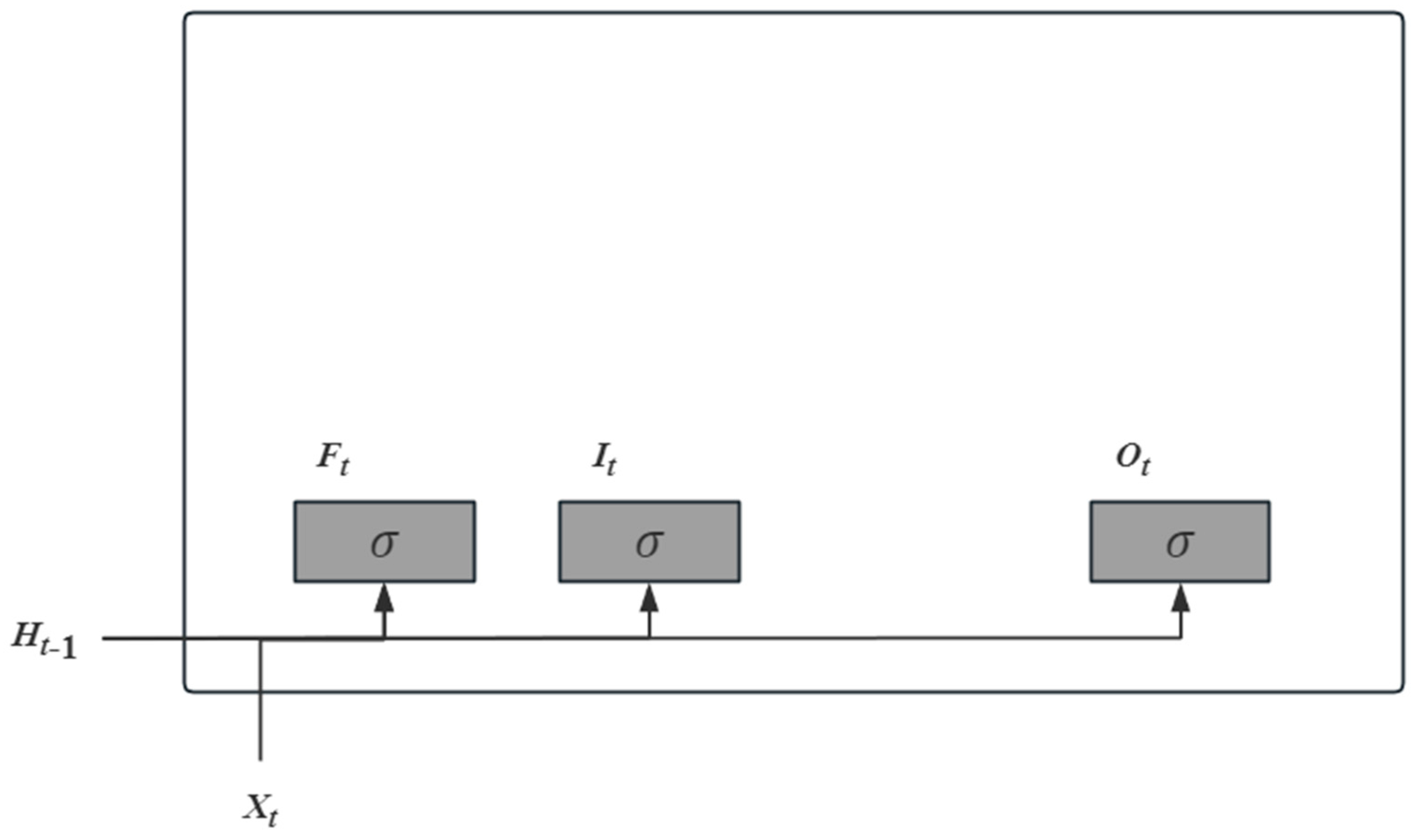
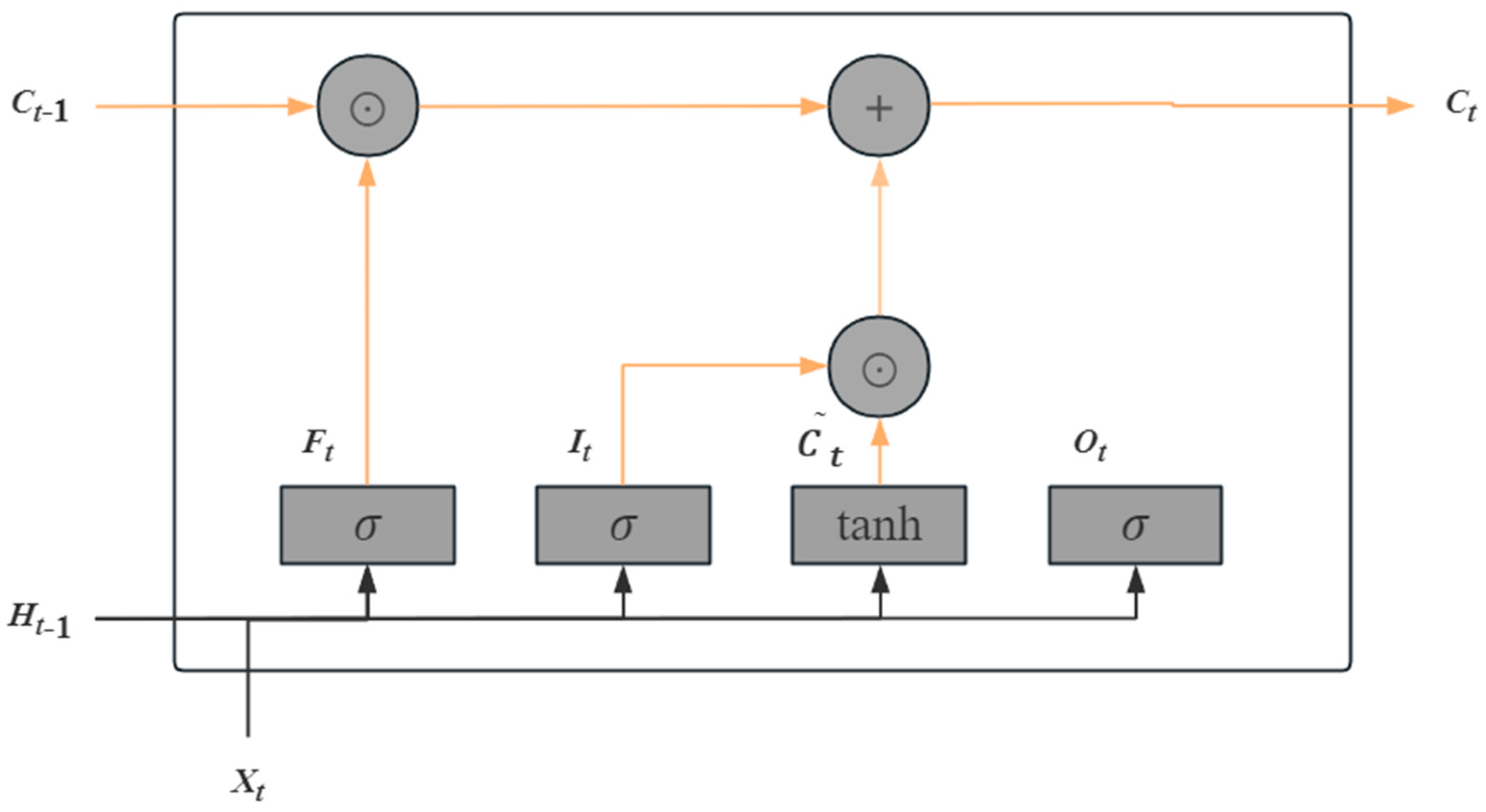
This study selects the LSTM network model, a gated recurrent neural network model, for forecasting. The basic principle is that the model has a recurrent unit in which the output of the previous moment is the input of the current moment, the output of the current moment is the input of the next moment, and a recurrent unit contains multiple components [25]. The specific process is divided into four parts. The first part is shown in Figure 1.

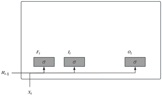
Figure 1. The first part of a single recurrent unit of the LSTM model.

According to the above figure, we have

$$\begin{array}{l}{I}_t=\sigma (X_t{W}_{xi}+H_{t-1}{W}_{hi}+b_i)\\ F_t=\sigma (X_t{W}_{xf}+H_{t-1}{W}_{hf}+b_f)\\ O_t=\sigma (X_t{W}_{xo}+H_{t-1}{W}_{ho}+b_o)\end{array}$$

(1)

$$\sigma (x)=\frac{1}{1+e^{-x}}$$

(2)

where the input X_t of the current step and the hidden state H_t−1 of the previous step will be sent into the input gate (I_t), forget gate (F_t), and output gate (O_t). X_t denotes the input data of the current step; the hidden state H_t−1 is the transformed result of the previous step, and the later H_t can be obtained later in the same way; W_x and W_h are the weights corresponding to the inputs and the hidden state, respectively; and each b represents bias, where all of them are parameters. The outputs of the three gates are obtained using the activation function, i.e., the sigmoid function (σ), which is used to transform the outputs nonlinearly. The second part is shown in Figure 2.

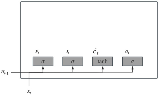
Figure 2. The second part of a single recurrent unit of the LSTM model.

According to the above figure, we have

$${\tilde{C}}_t=\tanh (X_t{W}_{xc}+H_{t-1}{W}_{hc}+b_c)$$

(3)

$$\tanh (x)=\frac{1-e^{-2x}}{1+e^{-2x}}$$

(4)

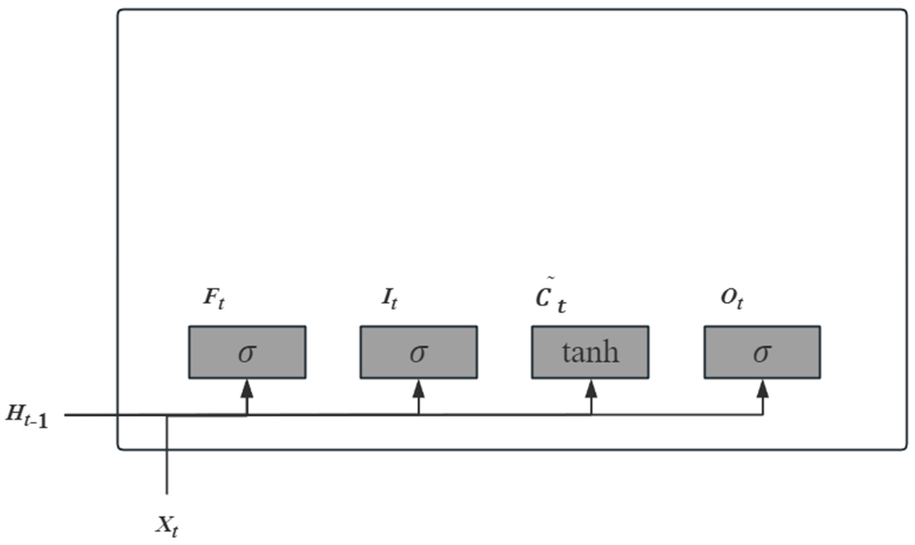
The LSTM requires calculating the candidate memory cell ${\tilde{C}}_t$, which is similar to the previous three gates but uses the tanh function as the activation function. After that, the third part is shown in Figure 3.

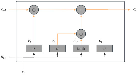
Figure 3. The third part of a single recurrent unit of the LSTM model.

According to the above figure, we have

$$C_t=F_t\odot C_{t-1}+I_t\odot {\tilde{C}}_t$$

(5)

The information flow in the hidden state is controlled by input gates, forget gates, and output gates with element domains in [0, 1]. The computation of the current step memory cell C_t combines the information of cell C_t−1 and the current step candidate memory cell and then controls the information flow through the forget gate and the input gate. The fourth part is shown in Figure 4.

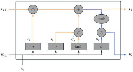
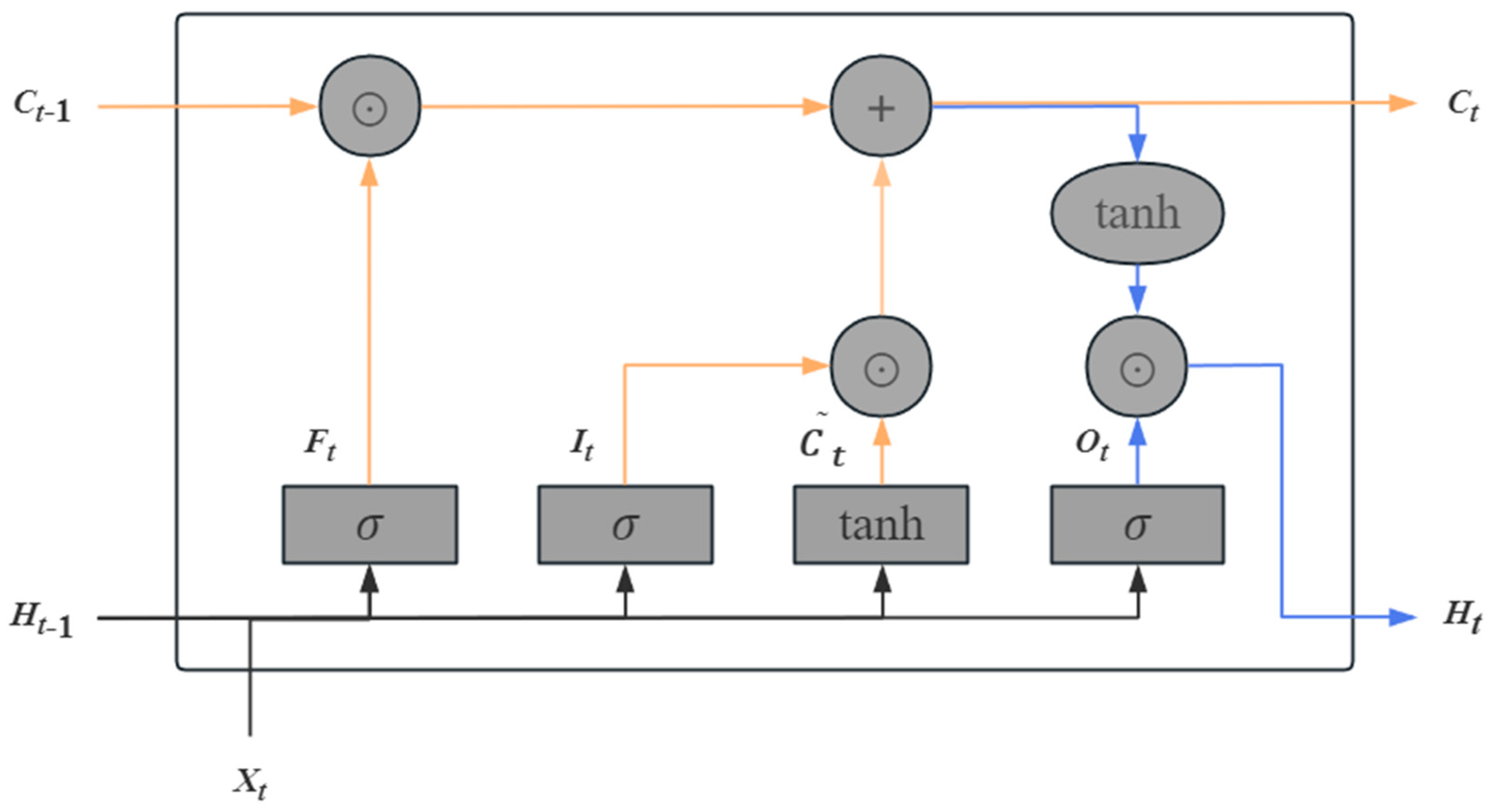
Figure 4. The fourth part of a single recurrent unit of the LSTM model.

According to the above figure, we have

$$H_t=O_t\odot \tanh (C_t)$$

(6)

With the memory cells, the information flow from the memory cells to the hidden state H_t is controlled by an output gate.

After the end of a cycle unit, the hidden state H_t updates parameters and weights with the loss function and optimization algorithm, which means one training is completed. The loss function with Adam’s optimization algorithm represents the mean square error.

The error(g_t) between the predicted value and the measurement is

$$g_t={({\widehat{y}}^{(i)}-y^{(i)})}^2$$

(7)

The optimization algorithm is used to iterate the parameters. The degree of parameter change in each training can be controlled by changing the learning rate. p_t (W_x, W_h, b) can be obtained using Adam’s algorithm as follows

$$\begin{array}{l}{v}_t={\gamma }_1{v}_{t-1}+(1-{\gamma }_1)g_t\\ s_t={\gamma }_2{s}_{t-1}+(1-{\gamma }_2)g_t\odot g_t\end{array}$$

(8)

$${\widehat{v}}_t=\frac{v_t}{1-{\gamma }_1^t},{\widehat{s}}_t=\frac{s_t}{1-{\gamma }_2^t}$$

(9)

$$\begin{array}{l}{\widehat{g}}_t=\frac{\eta {\widehat{v}}_t}{\sqrt{{\widehat{s}}_t}+\tau }\\ p_t=p_{t-1}-{\widehat{g}}_t\end{array}$$

(10)

where η is the learning rate and also a hyperparameter that needs to be set, and γ is a hyperparameter with domain [0, 1]. After the training set is put into the model and the training is complete, it is then put into the test set for forecasting, and the results are shown graphically against the exact values. The modeling error is expressed using the RMSE and the CC as follows,

$$\mathrm{RMSE}(X,h)=\sqrt{\frac{1}{m}{\displaystyle \sum _{i=1}^m{(h(x_i)-y_i)}^2}}$$

(11)

$$\mathrm{CC}=\frac{{\displaystyle \sum (x-\overline{x})(y-\overline{y})}}{\sqrt{{\displaystyle \sum {(x-\overline{x})}^2\cdot {\displaystyle \sum {(y-\overline{y})}^2}}}}$$

(12)

4.2. The EMD-LSTM Model

Another forecasting model used in this study is the EMD-LSTM model, which is a model that combines the Empirical Mode Decomposition (EMD) method with LSTM. The EMD was proposed by Huang et al. [26] to decompose signals into eigenmodes. The basic principle of the EMD algorithm is firstly find the maximum and minimum points of the original signal X(t) and then fit these extreme points using curve interpolation to obtain the upper envelope X_max(t) and lower envelope X_min(t) and finally determine the average of upper and lower values:

$$m_1(t)=\frac{X_{\max }(t)+X_{\min }(t)}{2}$$

(13)

The first intrinsic mode function (IMF) can be obtained by subtracting the original signal X(t) from the m₁(t), and the other IMFs can be obtained in the same way. Finally, the residual component (res) with only one extreme point that cannot be further decomposed can be acquired, which means the algorithm is finished. The core of the EMD algorithm is to decompose the original signal into several IMF components and one res component, which are of decreasing complexity. The sum of all these components is the original signal.

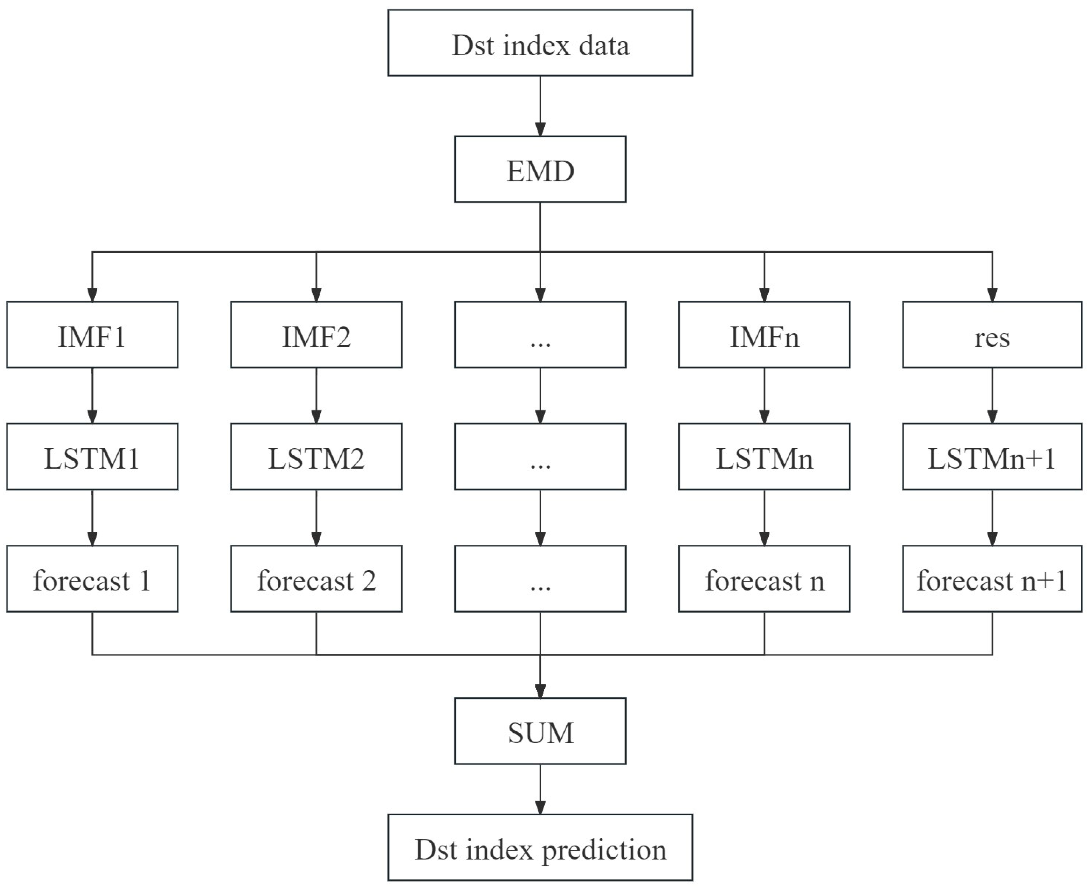
Compared with the LSTM algorithm, the EMD-LSTM is based on the idea that the EMD algorithm decomposes the training data and then puts the decomposed data into the LSTM model for training. Since most of the components derived from EMD decomposition have lower complexity, and LSTM can obtain better fitting results for them. So, the error of the final prediction result will be reduced to some extent. The working flow chart is shown in Figure 5.

Figure 5. The overall structure of the EMD-LSTM model.

In Figure 5, the training data are first decomposed using the EMD algorithm, then each component is trained using the LSTM model, merging all predictions to obtain the final prediction.

5. Results

After determining the modeling Dst data, the exact influences of different parameters on the prediction accuracy of the LSTM model are tested, and the parameters are also fixed for subsequent training. In order to test the validity and accuracy of the model, the Dst index is modeled and predicted for the solar quiet and active periods, respectively, and the consequent predictions are analyzed.

5.1. The Results of the Short-Period Prediction using the LSTM Model

First, we selected 90-day data (90 days since 1 January 2015) and 1096-day data (three years since 1 January 2015) as the training data to test the performance of the LSTM model for short-term (one-hour ahead) prediction, which aims to compare influences on the prediction accuracy at different learning rates and lengths of training data. The learning rate directly affects the degree of parameter changes after training; the more minor the parameter, the lower the amplitude of change during each training, and the more training times are needed to achieve the ideal fitting effect. Usually, the learning rate is chosen to be 10⁻³, 10⁻⁴, 10⁻⁵, or even smaller. Since the number of training times directly affects the training time, 10⁻³, 10⁻⁴, and 10⁻⁵ are the learning rates used to compare the prediction results. Here, we list the predictions based on 90 days with different learning rates and trainings.

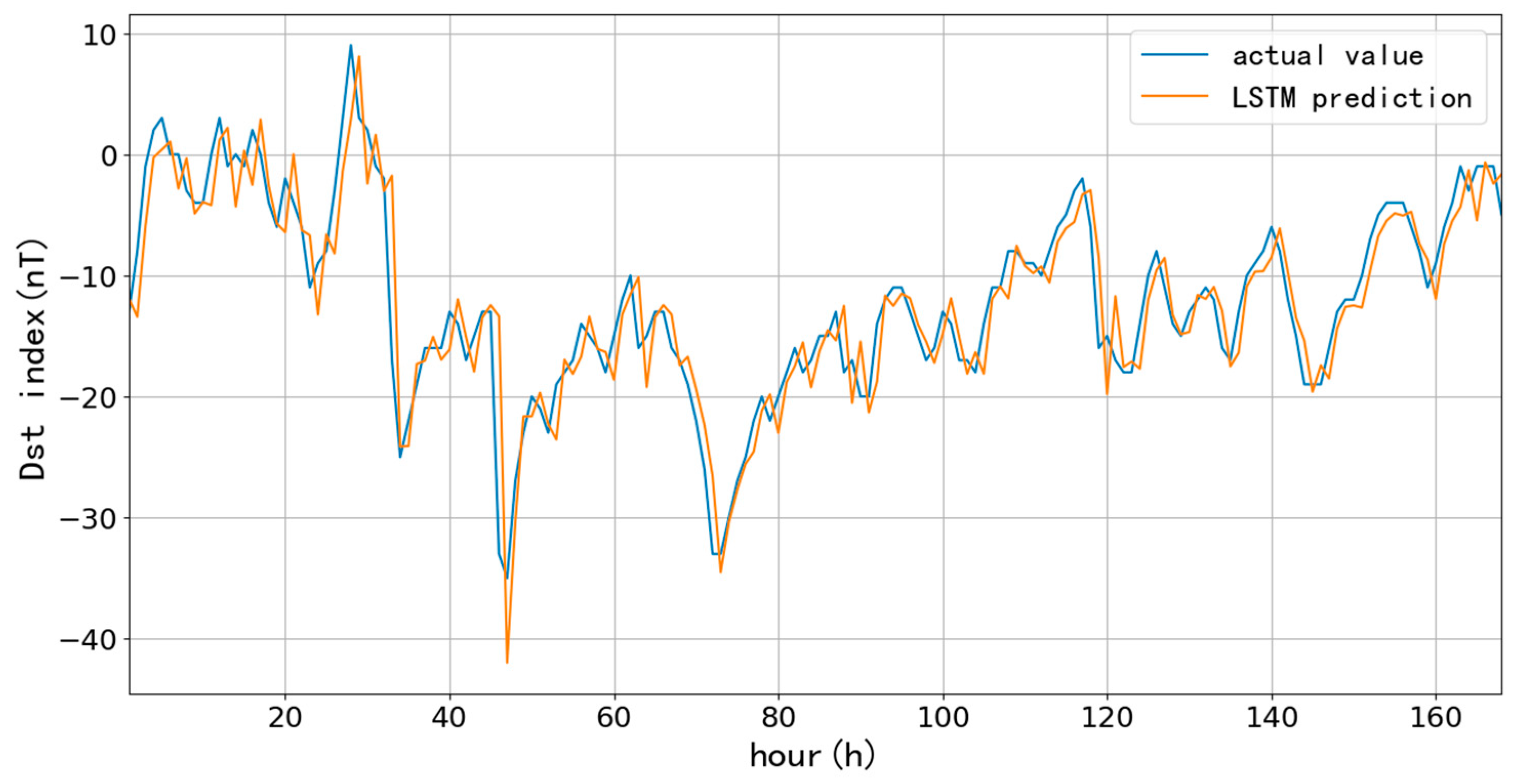
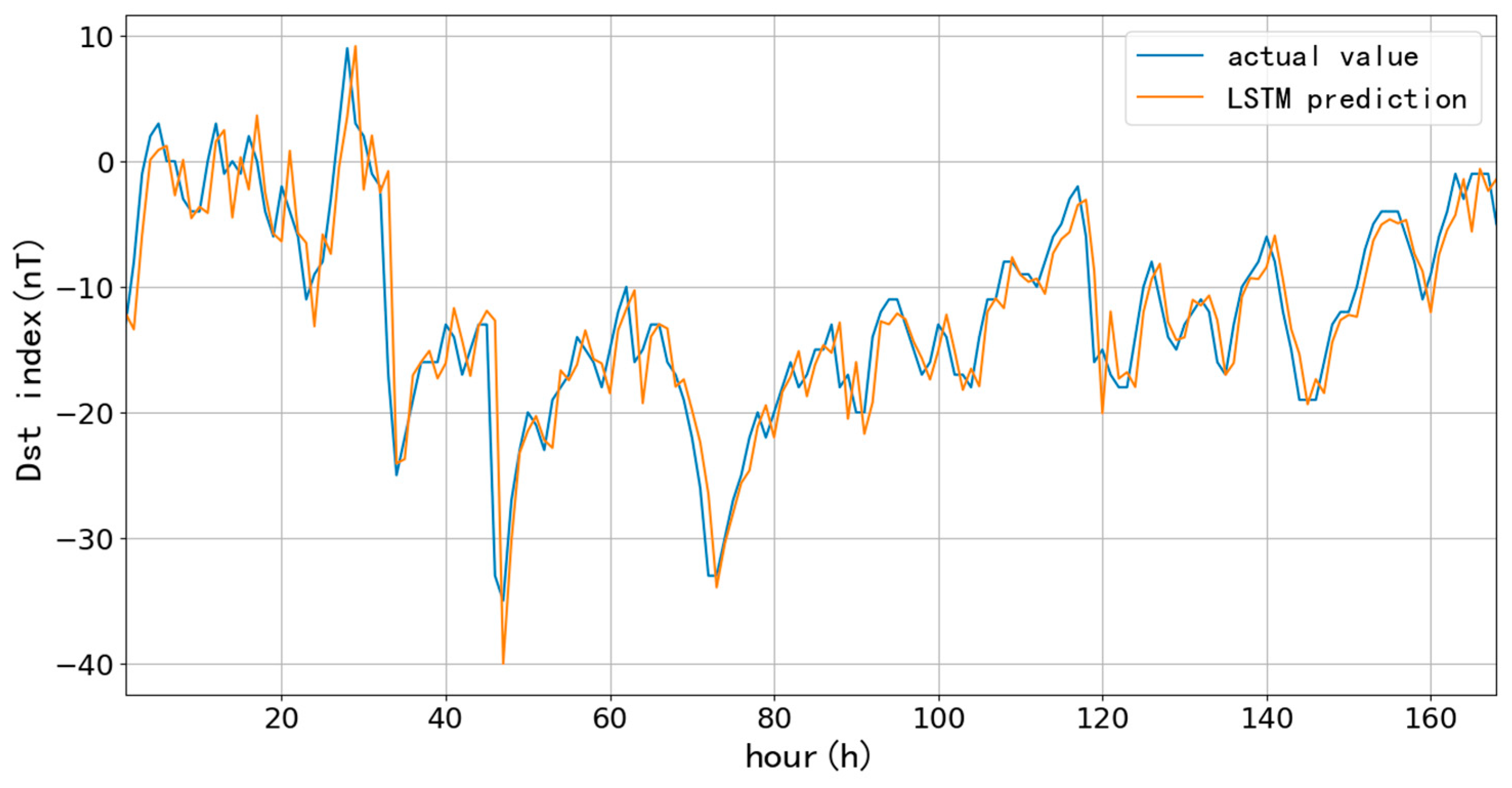
Figure 6, Figure 7 and Figure 8 and Table 2 show the one-hour ahead prediction of a 7-day length (168 h) using the 90-day data. As the learning rate decreases, the training number increases by around 400% to keep the close prediction error; the RMSE only decreases by 0.07 nT, the CC increases by 0.01, and the learning rate decreases from 10⁻³ to 10⁻⁵.

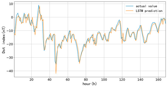
Figure 6. The model prediction through 650 trainings with a learning rate of 10⁻³.

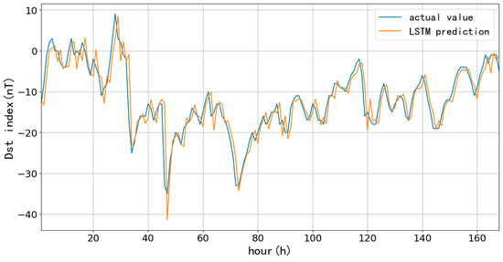
Figure 7. The model prediction through 3400 trainings with a learning rate of 10⁻⁴.

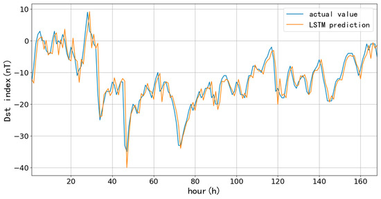
Figure 8. The model prediction through 20,000 trainings with a learning rate of 10⁻⁵.

Table 2. The 7-day length prediction using 90-day data.

Learning Rate	Trainings	RMSE (nT)	CC
10−3	650	3.27	0.91
10−4	3400	3.29	0.91
10−5	20,000	3.20	0.92

The predictions based on 1096-day data are as follows.

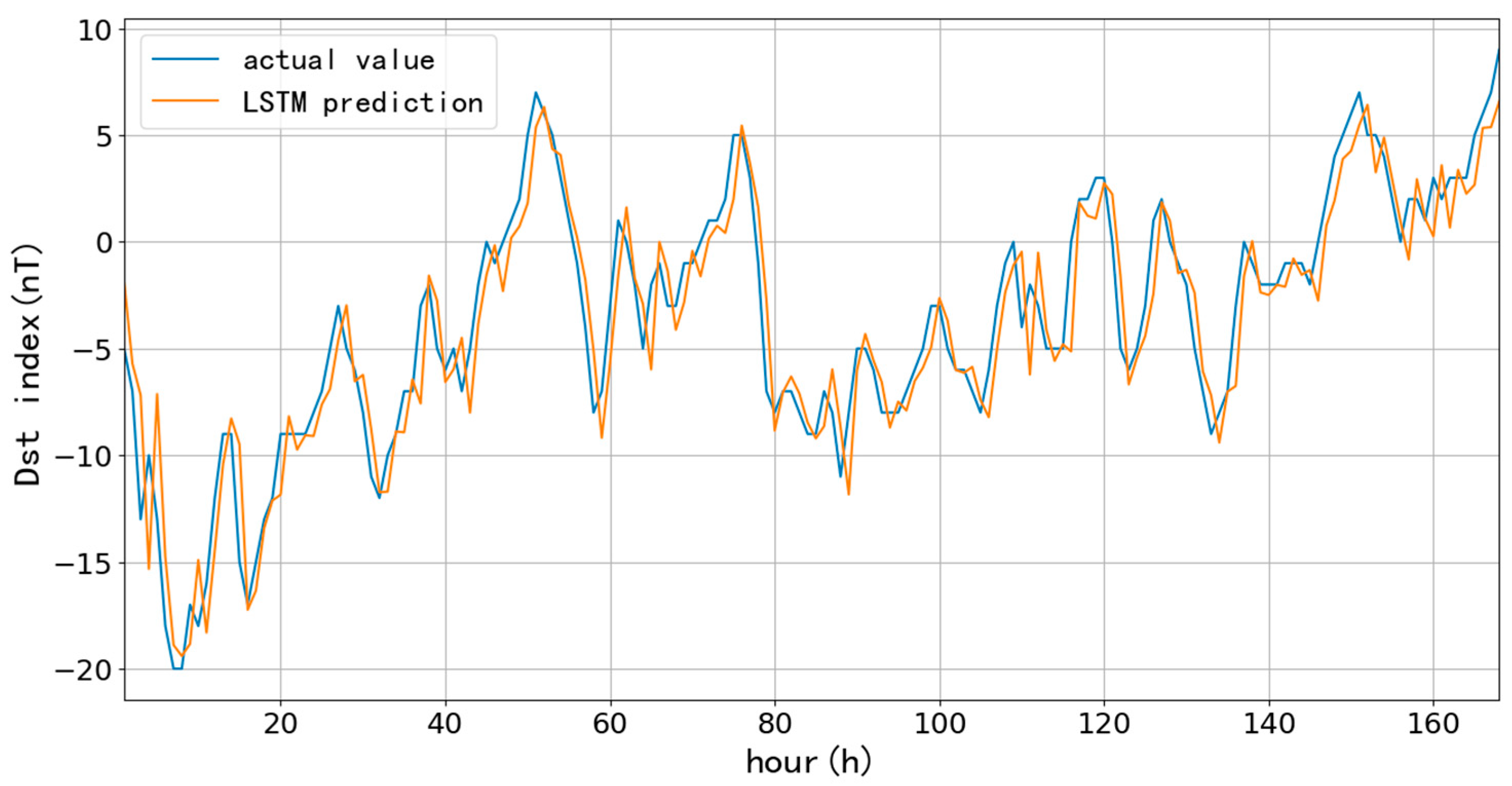
Figure 9, Figure 10 and Figure 11 and Table 3 show the one-hour ahead prediction results for a 7-day length using three years of data since 2015. The situation is similar to the 90-day results: the RMSE only decreases by 0.03 nT, while the learning rate changes from 10⁻³ to 10⁻⁵. In addition, the prediction error decreases by about 1.3 nT on average relative to the RMSE of the 90-day data, and the CC improves by 0.03, which suggests that increasing the prediction data can effectively improve the accuracy.

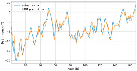
Figure 9. The model prediction through 650 trainings with a learning rate of 10⁻³.

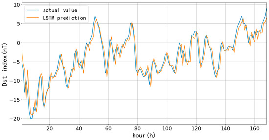
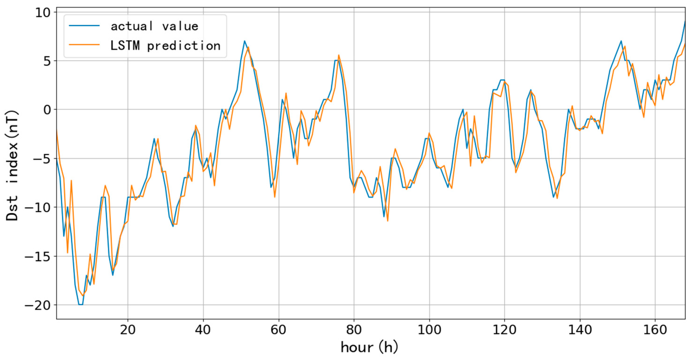
Figure 10. The model prediction through 3300 trainings with a learning rate of 10⁻⁴.

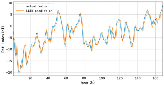
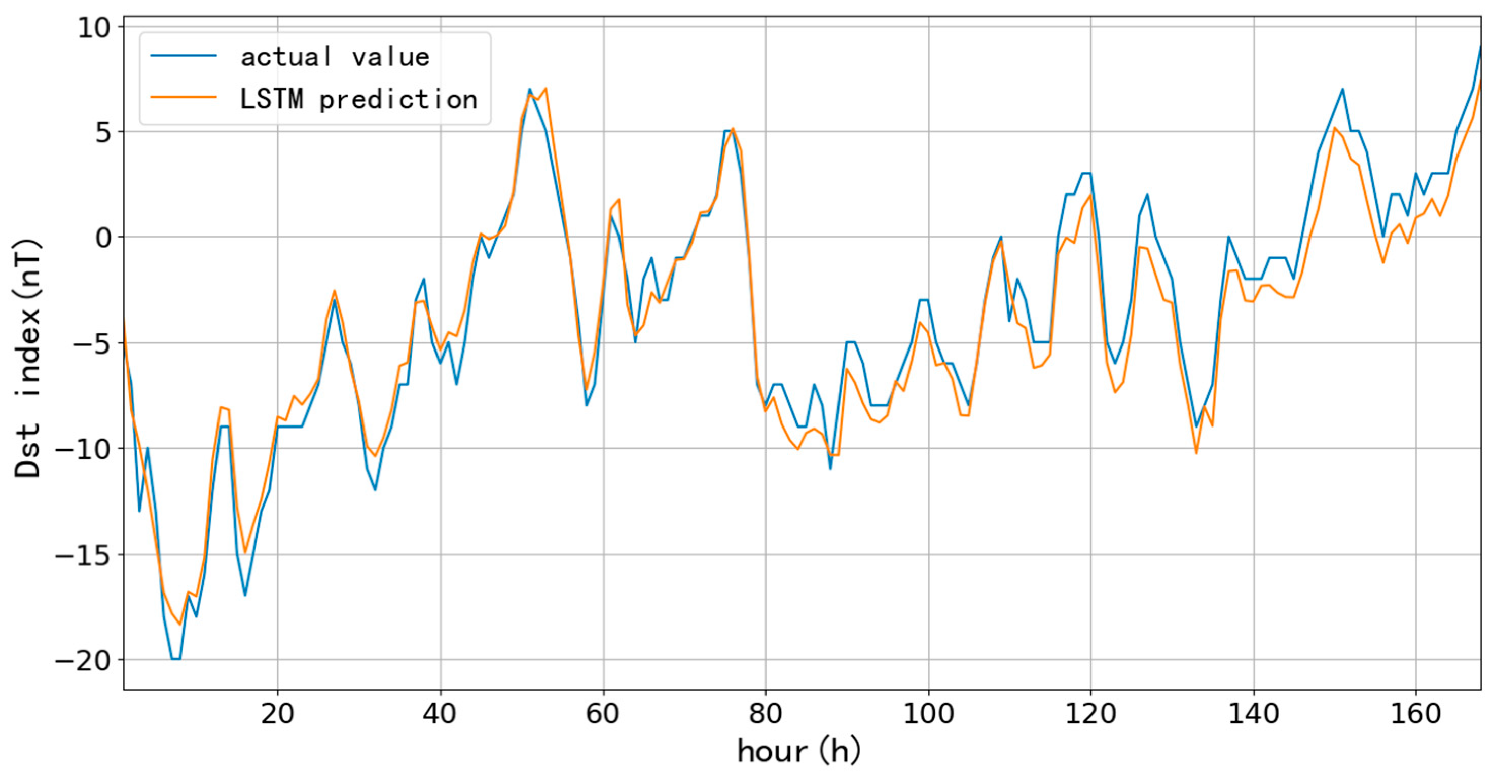
Figure 11. The model prediction through 18,000 trainings with a learning rate of 10⁻⁵.

Table 3. The 7-day length prediction using 1096-day data.

Learning Rate	Trainings	RMSE (nT)	CC
10−3	650	1.97	0.94
10−4	3300	1.95	0.94
10−5	18,000	1.94	0.94

However, the above figures show that the model-predicted values have a noticeable lag using different training data lengths. This lag phenomenon has also been observed in other studies using LSTM for prediction, such as Cai et al. [27] and Yin et al. [28]. This stems from the fact that when using the LSTM model for time-series prediction, the model algorithm is calculated using the values in the fixed time window as samples. In order to minimize the error, using the value at moment t as the prediction value of moment t + 1 not only requires no additional operations, but the error is very tiny, and the algorithm tends to use the value at moment t or t − 1 as the prediction value, thus generating a lag in the final prediction. Commonly used solutions include increasing the training data length and indirect prediction. To take advantage of the feature of the EMD-LSTM method and obtain segmented average values and then perform LSTM prediction, we use Figure 9 as an example and perform tests as follows.

In Figure 12, under the same conditions as in Figure 9, using the EMD-LSTM model, the original data are decomposed into 14 components using the EMD algorithm, which are individually predicted with LSTM fitting and finally merged to obtain the prediction results. The EMD-LSTM model fits better than the LSTM model because the EMD algorithm can split the data series by detecting the peak and valley values of the two curves, which directly and effectively improves the lag in the prediction.

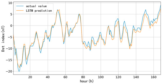
Figure 12. Results of the EMD-LSTM model when using the same parameters as in Figure 9.

According to the above tests, a lower learning rate has few accuracy improvements. At the same time, the training times and training time increased significantly, so we chose a learning rate of 10⁻³ for subsequent model training.

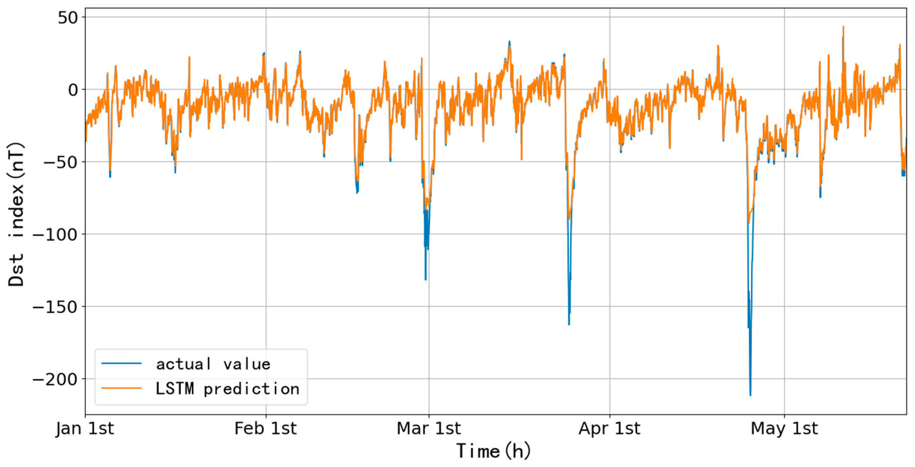
By observing the actual Dst data, the data from 2019 are selected as the test set to predict the quiet period, and the data from 1 January 2023 to 21 May are selected as the test set for the active period prediction. The results are as follows.

Figure 13 shows the results of using the 2018 Dst data with one-hour ahead forecasting for 2019. The results show that the fitted values agree well with the actual values. The RMSE is 2.64 nT, the CC is 0.97, and the precision of the results is between those obtained by LSTM using 90 and 1096 days of data.

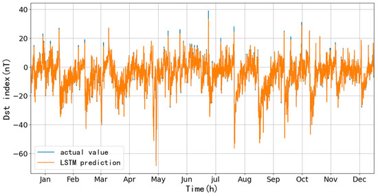
Figure 13. Results of model prediction through 750 training sessions at a learning rate of 10⁻³.

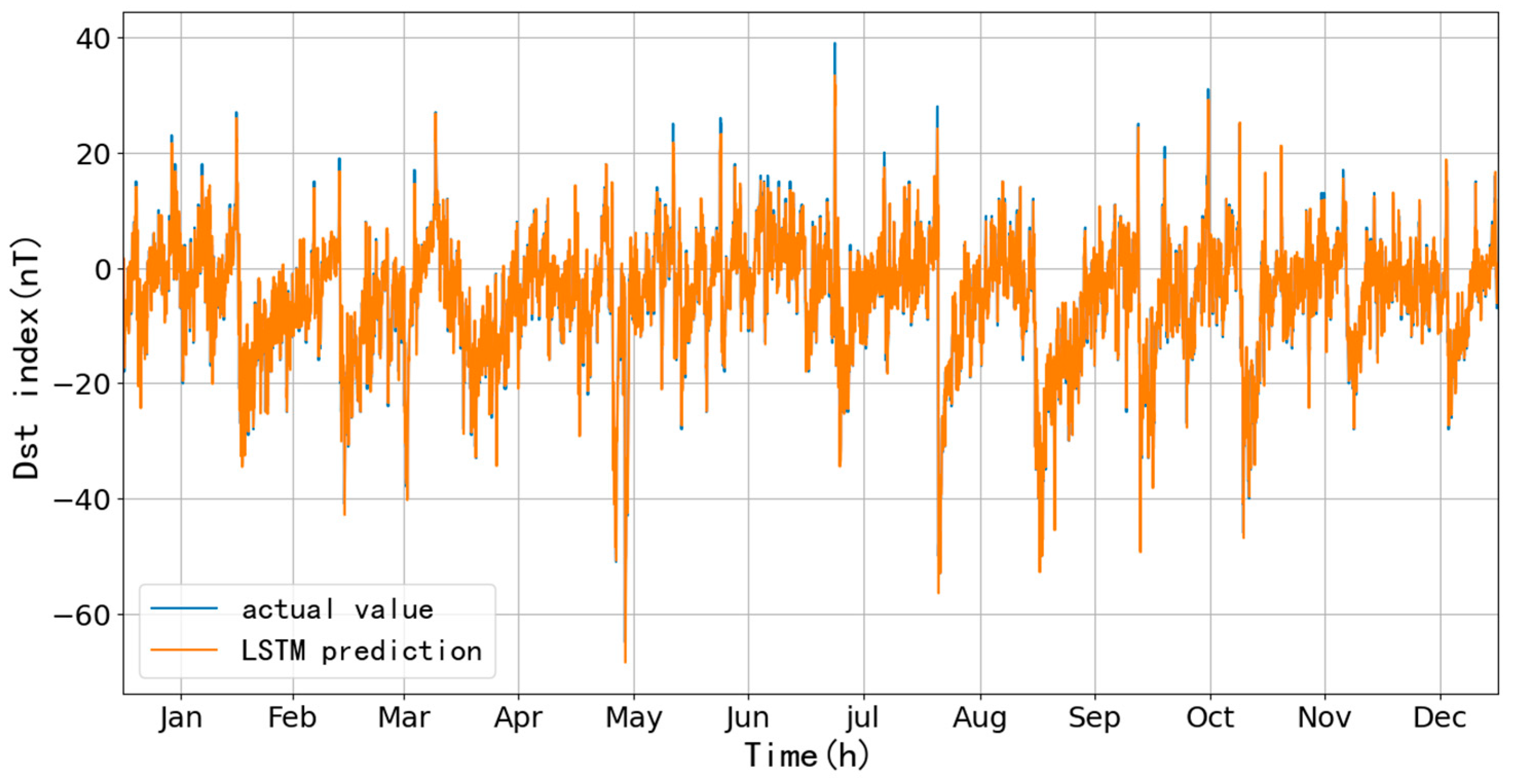
In order to further test the model, the dramatic changes in the Dst index in 2023 are now predicted based on the 2022 data, and we expect to model and predict the corresponding geomagnetic storms. The following are the results based on the LSTM model.

Figure 14 shows the one-hour ahead prediction of the data from 1 January to 21 May 2023, with an RMSE of 7.34 nT and a CC of 0.96, using the Dst data of 2022. The storm with the largest amplitude occurred on 24 April, and its prediction results are shown in Figure 15, with an RMSE of 20.47 nT and a CC of 0.91 before and after the storm (300 h). It is found that the fitting before and after the storm valley is good, while the prediction of the main phase is not good, and the difference is more than 100 nT.

Figure 14. The model prediction through 750 trainings with a learning rate of 10⁻³.

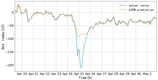
Figure 15. Predictions before and after the 24 April 2023 geomagnetic storm.

5.2. The Results of the Short-Period Prediction Using the EMD-LSTM Model

In order to effectively solve the time lag problem and to improve the accuracy of the prediction, the EMD-LSTM method is used to predict the Dst index in 2019 and 2023. The following is part of the forecast results for the quiet period.

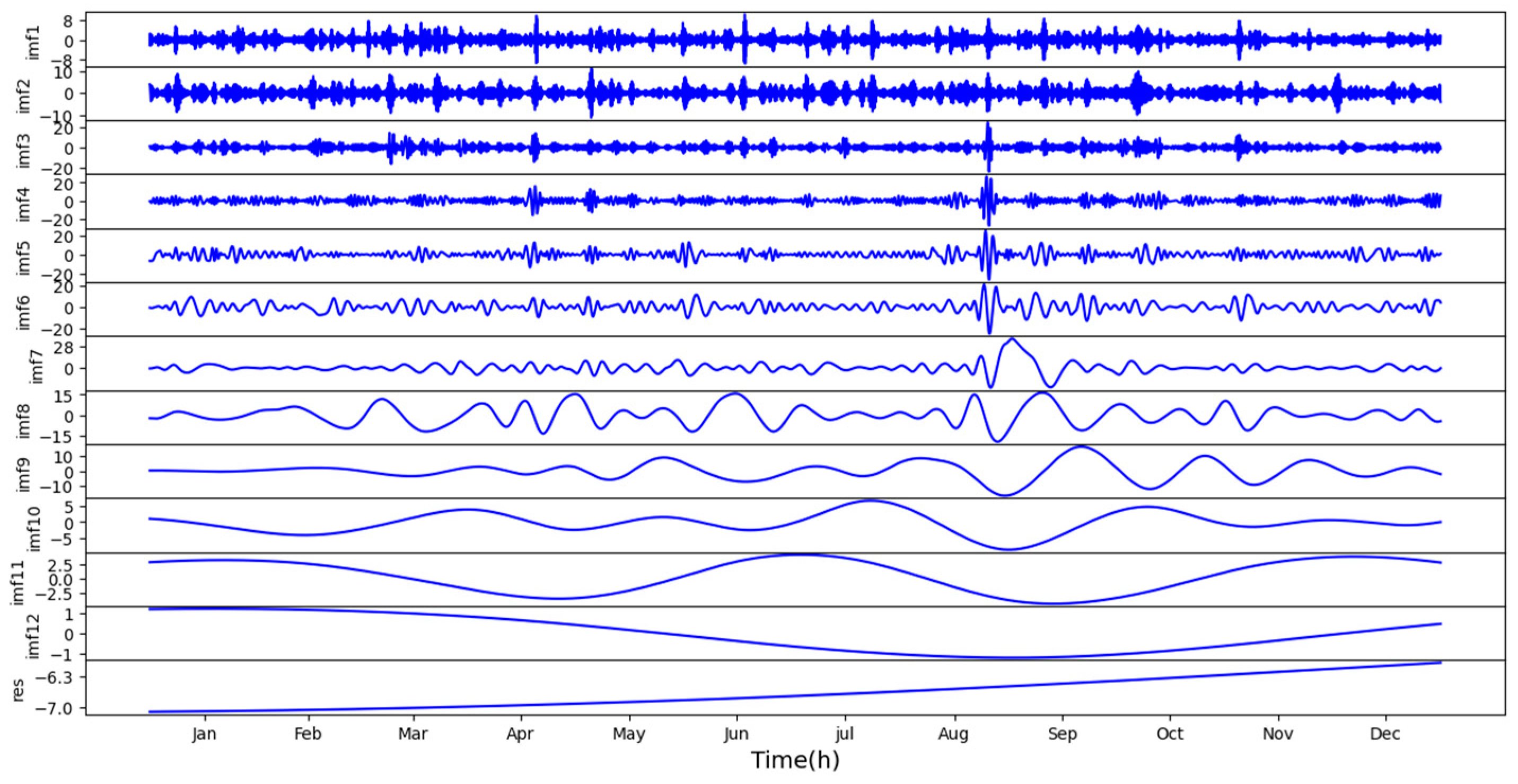
Figure 16 shows that the EMD algorithm mathematically decomposes the original Dst index data into several wavelength components. Each part possesses different characteristics (determined using the original data), and the complexity of these components decreases in order. The error during model training is mainly concentrated in the first few components rather than the entire Dst index, so using EMD-LSTM can make the prediction closer to the actual value.

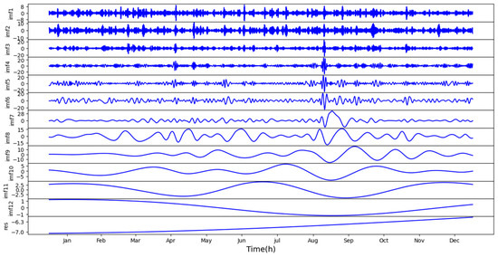
Figure 16. Data decomposition using EMD based on the 2018 Dst index.

We first predict the data from 2019.

Figure 17 shows the result of using the Dst data from 2018, making a one-hour ahead prediction and predicting the data from 2019. The RMSE is 3.29 nT, and the CC is 0.95, which makes the prediction effect more satisfactory. Compared with the LSTM method, the RMSE increased by 0.65 nT and the CC decreased by 0.02.

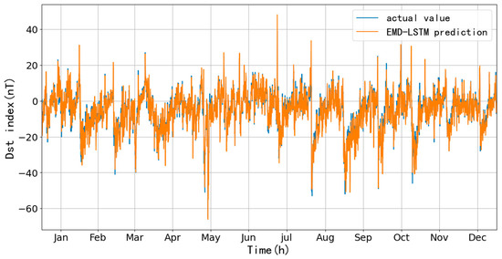
Figure 17. Results of model prediction through 600 training sessions with a learning rate of 10⁻³.

Next, we test the prediction for 2023.

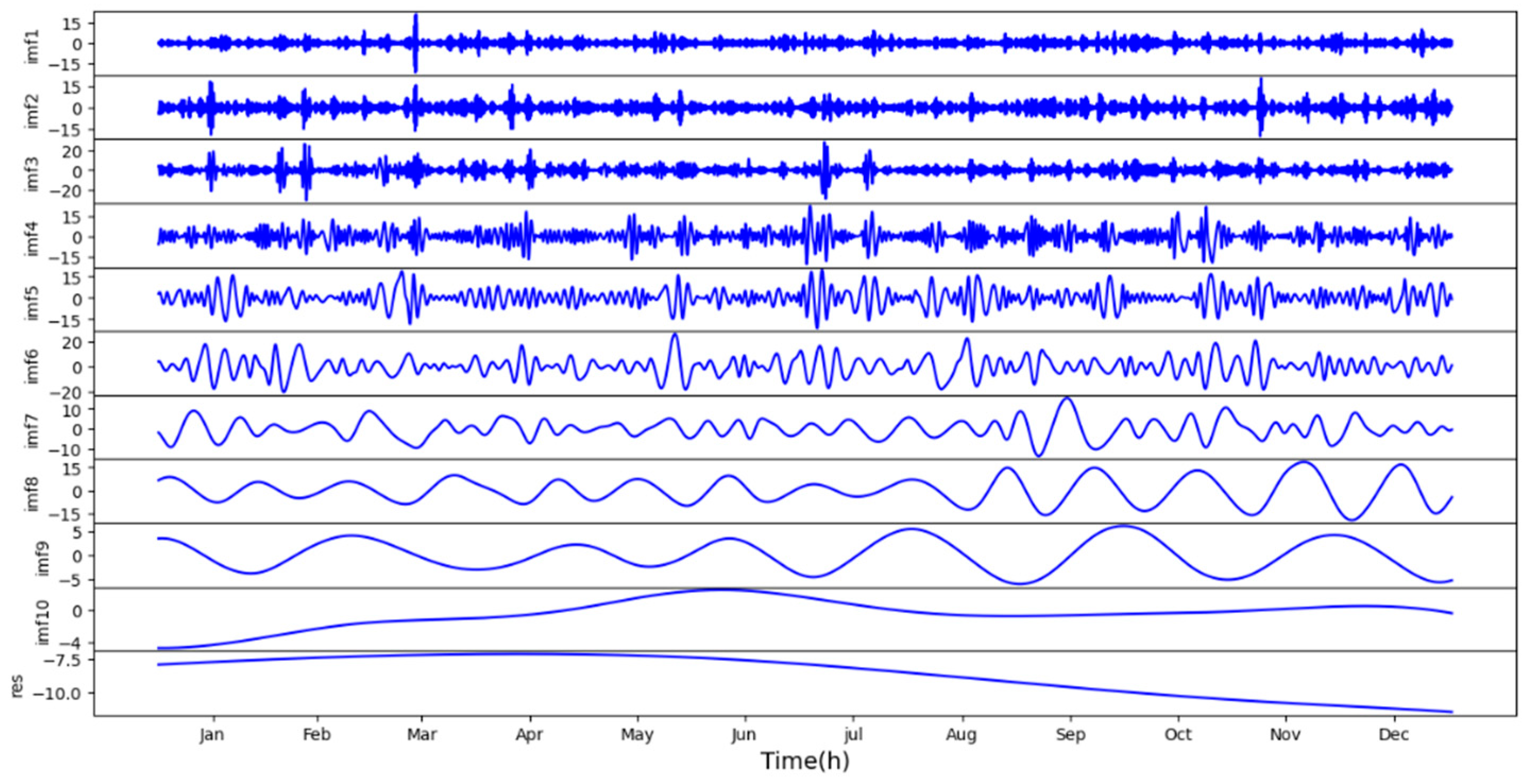
Figure 18 shows different parts of the 2022 Dst index decomposed using EMD.

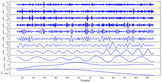
Figure 18. Results of the Dst index data decomposition using the EMD method for 2022.

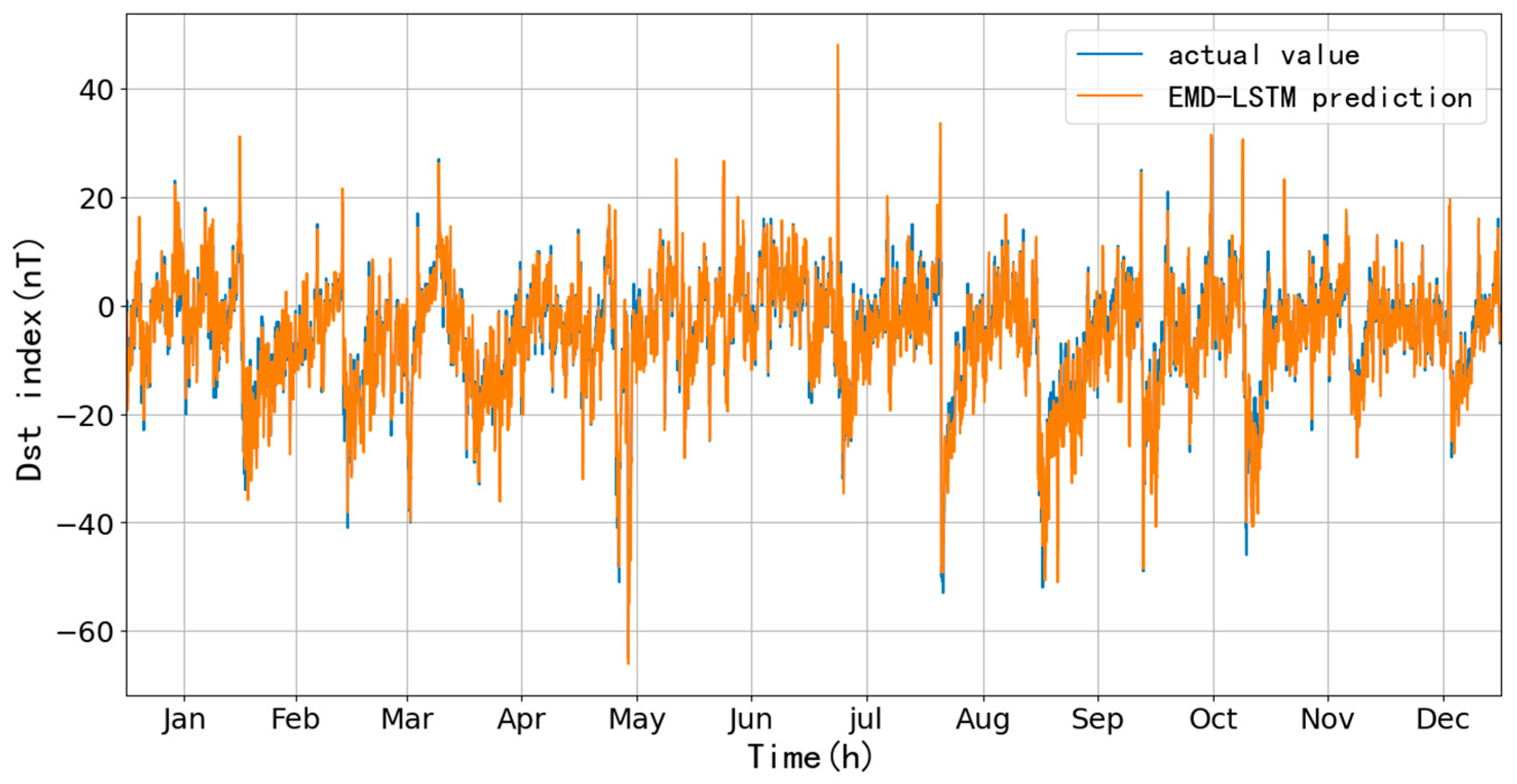
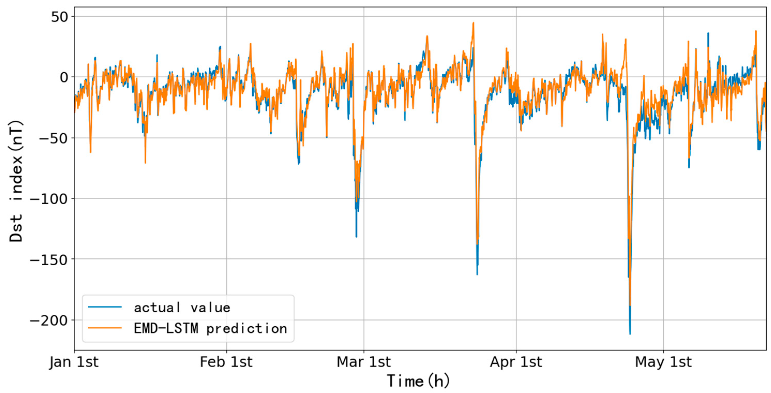
Figure 19 shows a one-hour ahead prediction from 1 January to 21 May 2023 using the 2022 Dst data. The results show that the RMSE is 8.87 nT and the CC is 0.93. There is an increase of 1.53 nT in the RMSE and a decrease of 0.03 in the CC compared with the LSTM method, and the fitting of the main phase is obviously better than the LSTM method.

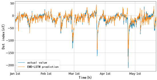
Figure 19. The model prediction through 650 trainings with a learning rate of 10⁻³.

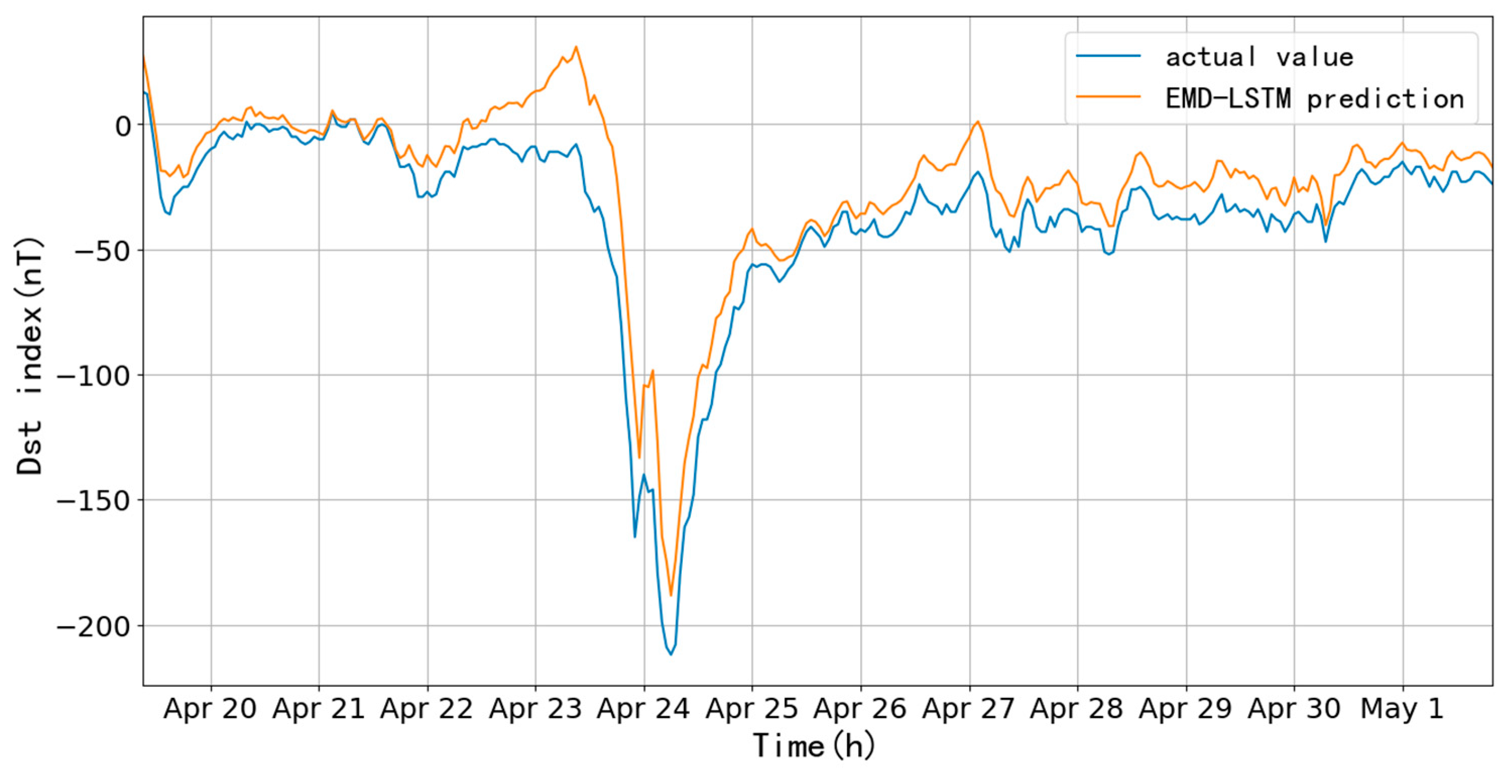
For further inspection, we list the modeling of the geomagnetic storm that occurred on 24 April 2023.

Figure 20 shows that the modeling is highly consistent in the start timing, amplitude, and recovery value of the magnetic storm. In the period before and after the storm (300 h), the RMSE is 16.91 nT and the CC is 0.96; they reduced by 3.56 nT and improved by 0.05 compared with the LSTM model. The fitted values are slightly higher during the initial and main phases, while they are more consistent during the recovery phase. The Dst index during the main phase can be effectively and precisely predicted. In addition, the lag in the predicted values is greatly improved by the indirect prediction with the decomposition of the original data using the EMD algorithm.

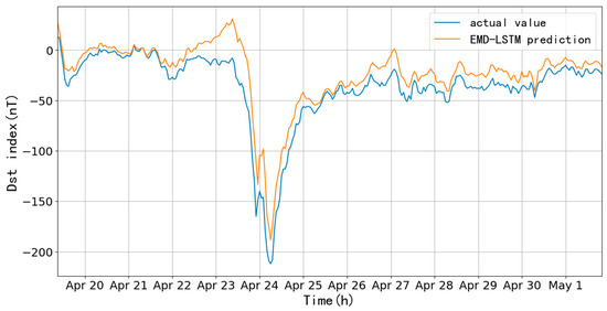
Figure 20. Predictions of the geomagnetic storm that occurred on 24 April 2023.

Comparing the two methods, from the viewpoint of the RMSE and CC, LSTM is slightly better than EMD-LSTM, but EMD-LSTM is better during the magnetic storm.

6. Conclusions

In this study, we trained and predicted the LSTM and EMD-LSTM models by observing and comparing the exact Dst index and selecting appropriate data segments. The factors affecting the prediction accuracy of the LSTM model were first tested, and the parameters used in the LSTM model were determined. Then, the two models were used to predict the Dst index for the quiet and active periods. After analyzing the prediction results, the related conclusions are reached as follows:

(1)

In predicting the Dst index using the LSTM model, a decrease in the learning rate and an increase in the number of training times have no significant influences on improving the prediction accuracy. When using 90-day length data for 7-day prediction, the change in the RMSE is within 0.1 nT and the CC varies around 0.01 under different learning rates. The change in the RMSE is within 0.05 nT and the CC does not change when using 1096-day data, whereas increasing the training data length can improve the prediction accuracy. The prediction accuracy can be improved by increasing the length of the training data: the RMSE decreases from an average of 3.25 nT to 1.95 nT and the CC improves from 0.91 to 0.94 when using 1096 days of data, which suggests that the base dataset is a critical factor in controlling the prediction.

(2)

The LSTM and EMD-LSTM models have better Dst prediction for the quiet period than the active period. The reason is that the fluctuation in the Dst index during the quiet period is slight (±50 nT), so the resulting model based on higher temporal resolution (time-averaged) is robust. The interferences from other factors, especially the solar activity, are less in the quiet period; combining the appropriate training rate and training times can predict the Dst changes better. During geomagnetic storms, the fluctuation amplitude in Dst caused by the solar wind can reach several hundred nT or more. Compared with the use of the LSTM model, the error is significantly reduced when training data are decomposed using the EMD algorithm and then put into the LSTM training, particularly during the big magnetic storm, but the overall prediction accuracy is lower than that of LSTM.

(3)

Although the overall prediction accuracy of the LSTM model is slightly higher than the EMD-LSTM model (the RMSE is reduced by about 1.5 nT and the CC is improved by about 0.03), there is a noticeable lag in the prediction results of the former. EMD-LSTM significantly improves the lag in the prediction results of LSTM. In addition, the prediction accuracy of EMD-LSTM during magnetic storms is better than that of LSTM. In practical applications, it is appropriate to select a suitable model by referencing the intensity of solar activity, such as the sunspot number, and if its value is high, the EMD-LSTM model can be chosen, or the LSTM model can be chosen if the situation is opposite. If the error requirement is not strict, using the LSTM method with a higher learning rate is economical to reduce the computation amount and satisfy the accuracy requirement.

7. Discussion

We tested the LSTM and EMD-LSTM models in terms of their ability for Dst index prediction. Our results prove the effectiveness of deep learning methods, which can be used to improve the prediction accuracy of the model by changing the model parameters and length of the training data, processing the training data, replacing the training data. Thus, this method is worthy of deeper study in the future. The newly launched MSS-1 satellite [29], which provides high accuracy and nearly east–west oriented (inclination angle of 41°) magnetic field data, can lay a solid foundation for studying the removal of external field interference and even for studying short-term changes in the ionospheric field and the magnetospheric ring current.

There are also some shortcomings in this study. The models only use one kind of data for training and prediction and lack the necessary physical constraints. Thus, the next step will be to screen other space weather indices and select indices with higher correlation with the Dst index, such as the magnetospheric ring current index (RC index) or the geomagnetic perturbation index (Ap index), for constraints and co-estimating, using multiple input parameters for training and predicting. In this way, realistic prediction results can be obtained by adding physical constraints.

References

- Sugiura, M. Hourly values of equatorial Dst for the IGY. Ann. Int. Geophys. Year 1964, 35, 9–45. [Google Scholar]
- Wu, Y.Y. Problems and thoughts on the Dst index of geomagnetic activity. Adv. Geophys. 2022, 37, 1512–1519. [Google Scholar]
- Tran, Q.A.; Sołowski, W.; Berzins, M.; Guilkey, J. A convected particle least square interpolation material point method. Int. J. Numer. Methods Eng. 2020, 121, 1068–1100. [Google Scholar] [CrossRef]
- Sun, Z.J.; Xue, L.; Xu, Y.M.; Wang, Z. A review of deep learning research. Comput. Appl. Res. 2012, 29, 2806–2810. [Google Scholar]
- Hochreiter, S.; Schmidhuber, J. Long short-term memory. Neural Comput. 1997, 9, 1735–1780. [Google Scholar] [CrossRef] [PubMed]
- Yang, L.; Wu, Y.X.; Wang, J.L.; Liu, Y.L. A review of recurrent neural network research. Comput. Appl. 2018, 38, 1–6+26. [Google Scholar]
- Liu, J.Y.; Shen, C.L. Forecasting Dst index using artificial intelligence method. In China Earth Science Joint Academic Conference, Proceedings of the 2021 China Joint Academic Conference on Earth Sciences (I)-Topic I Solar Activity and Its Space Weather Effects, Topic II Plasma Physical Processes in the Magnetosphere, Topic III Planetary Physics, Zhuhai, China, 11–14 November 2021; Beijing Berton Electronic Publishing House: Beijing, China, 2021; p. 12. [Google Scholar] [CrossRef]
- Kim, R.S.; Cho, K.S.; Moon, Y.J.; Dryer, M.; Lee, J.; Yi, Y.; Kim, K.H.; Wang, H.; Park, Y.D.; Kim, Y.H. An empirical model for prediction of geomagnetic storms using initially observed CME parameters at the Sun. J. Geophys. 2010, 115, A12108. [Google Scholar] [CrossRef]
- Kremenetskiy, I.A.; Salnikov, N.N. Minimax Approach to Magnetic Storms Forecasting (Dst-index Forecasting). J. Autom. Inf. Sci. 2011, 3, 67–82. [Google Scholar] [CrossRef]
- Tobiska, W.K.; Knipp, D.; Burke, W.J.; Bouwer, D.; Bailey, J.; Odstrcil, D.; Hagan, M.P.; Gannon, J.; Bowman, B.R. The Anemomilos prediction methodology for Dst. Space Weather 2013, 11, 490–508. [Google Scholar] [CrossRef]
- Banerjee, A.; Bej, A.; Chatterjee, T.N. A cellular automata-based model of Earth’s magnetosphere in relation with Dst index. Space Weather 2015, 13, 259–270. [Google Scholar] [CrossRef]
- Chandorkar, M.; Camporeale, E.; Wing, S. Probabilistic forecasting of the disturbance storm time index: An autoregressive Gaussian process approach. Space Weather 2017, 15, 1004–1019. [Google Scholar] [CrossRef]
- Bej, A.; Banerjee, A.; Chatterjee, T.N.; Majumdar, A. One-hour ahead prediction of the Dst index based on the optimum state space reconstruction and pattern recognition. Eur. Phys. J. Plus 2022, 137, 479. [Google Scholar] [CrossRef]
- Nilam, B.; Tulasi Ram, S. Forecasting Geomagnetic activity (Dst Index) using the ensemble kalman filter. Mon. Not. R. Astron. Soc. 2022, 511, 723–731. [Google Scholar] [CrossRef]
- Chen, C.; Sun, S.J.; Xu, Z.W.; Zhao, Z.W.; Wu, Z.S. Forecasting Dst index one hour in advance using neural network technique. J. Space Sci. 2011, 31, 182–186. [Google Scholar] [CrossRef]
- Revallo, M.; Valach, F.; Hejda, P.; Bochníček, J. A neural network Dst index model driven by input time histories of the solar wind–magnetosphere interaction. J. Atmos. Sol.-Terr. Phys. 2014, 110–111, 9–14. [Google Scholar] [CrossRef]
- Lu, J.Y.; Peng, Y.X.; Wang, M.; Gu, S.J.; Zhao, M.X. Support Vector Machine combined with Distance Correlation learning for Dst forecasting during intense geomagnetic storms. Planet. Space Sci. 2016, 120, 48–55. [Google Scholar] [CrossRef]
- Andriyas, T.; Andriyas, S. Use of Multivariate Relevance Vector Machines in forecasting multiple geomagnetic indices. J. Atmos. Sol.-Terr. Phys. 2017, 154, 21–32. [Google Scholar] [CrossRef]
- Lethy, A.; El-Eraki, M.A.; Samy, A.; Deebes, H.A. Prediction of the Dst index and analysis of its dependence on solar wind parameters using neural network. Space Weather 2018, 16, 1277–1290. [Google Scholar] [CrossRef]
- Xu, S.; Huang, S.; Yuan, Z.; Deng, X.; Jiang, K. Prediction of the Dst index with bagging ensemble-learning algorithm. Astrophys. J. Suppl. Ser. 2020, 248, 14. [Google Scholar] [CrossRef]
- Park, W.; Lee, J.; Kim, K.C.; Lee, J.; Park, K.; Miyashita, Y.; Sohn, J.; Park, J.; Kwak, Y.S.; Hwang, J.; et al. Operational Dst index prediction model based on combination of artificial neural network and empirical model. J. Space Weather Space Clim. 2021, 11, 38. [Google Scholar] [CrossRef]
- Hu, A.; Shneider, C.; Tiwari, A.; Camporeale, E. Probabilistic prediction of Dst storms one-day-ahead using full-disk SoHO images. Space Weather 2022, 20, e2022SW003064. [Google Scholar] [CrossRef]
- Finlay, C.C.; Kloss, C.; Olsen, N.; Hammer, M.D.; Tøffner-Clausen, L.; Grayver, A.; Kuvshinov, A. The CHAOS-7 geomagnetic field model and observed changes in the South Atlantic Anomaly. Earth Planets Space 2020, 156, 72. [Google Scholar] [CrossRef] [PubMed]
- Zhang, H.; Xu, H.R.; Peng, G.S.; Qian, Y.D.; Zhang, X.X.; Yang, G.L.; Shen, C.; Li, Z.; Yang, J.W.; Wang, Z.Q.; et al. A prediction model of relativistic electrons at geostationary orbit using the EMD-LSTM network and geomagnetic indices. Space Weather 2022, 20, e2022SW003126. [Google Scholar] [CrossRef]
- Graves, A.; Schmidhuber, J. Framewise phoneme classification with bidirectional LSTM and other neural network architectures. Neural Netw. 2005, 18, 5–6. [Google Scholar] [CrossRef] [PubMed]
- Huang, N.E.; Shen, Z.; Long, S.R.; Wu, M.C.; Shih, H.H.; Zheng, Q.; Yen, N.C.; Tung, C.C.; Liu, H.H. The empirical mode decomposition and the Hilbert spectrum for nonlinear and non-stationary time series analysis. Proc. R. Soc. Lond. A Mat. Proc. Math. Phys. Eng. Sci. 1998, 454, 903–995. [Google Scholar] [CrossRef]
- Cai, J.; Dai, X.; Hong, L.; Gao, Z.; Qiu, Z. An air quality prediction model based on a noise reduction self-coding deep network. Math. Probl. Eng. 2020, 2020, 3507197. [Google Scholar] [CrossRef]
- Yin, H.; Jin, D.; Gu, Y.H.; Park, C.J.; Han, S.K.; Yoo, S.J. STL-ATTLSTM: Vegetable Price Forecasting Using STL and Attention Mechanism-Based LSTM. Agriculture 2020, 10, 612. [Google Scholar] [CrossRef]
- Zhang, K. A novel geomagnetic satellite constellation: Science and applications. Earth Planet. Phys. 2023, 7, 4–21. [Google Scholar] [CrossRef]
Disclaimer/Publisher’s Note: The statements, opinions and data contained in all publications are solely those of the individual author(s) and contributor(s) and not of MDPI and/or the editor(s). MDPI and/or the editor(s) disclaim responsibility for any injury to people or property resulting from any ideas, methods, instructions or products referred to in the content. |
© 2023 by the authors. Licensee MDPI, Basel, Switzerland. This article is an open access article distributed under the terms and conditions of the Creative Commons Attribution (CC BY) license (https://creativecommons.org/licenses/by/4.0/).