A Modified Model for Identifying the Characteristic Parameters of Machine Joint Interfaces

Abstract

The contact parameters of joint interfaces have a great influence on the dynamic performance of the machine tool, and the dynamic performance determines the machining precision of the machine tool. Therefore, it is important to accurately identify the contact parameters of joint interfaces to improve the machining precision of the machine tool. In this paper, a method of identifying the joint interface stiffness parameters based on a joint simulation in Matlab and Ansys is first proposed, and then stiffness parameters of joint interfaces between the bed and column of the precision grinding machine are identified by applying the method. Finally, the feasibility and high efficiency of the proposed method are proved by comparing the natural frequencies of the simulation and the experiment. In order to further analyze the influence of joint contact parameters on the performance of the joint interfaces, the theoretical model of the normal stiffness of the joint interfaces based on fractal geometry is amended and verified by taking into account the asperity interaction and elastic–plastic deformation. Then, the modified model is extended to a three-dimensional model, which is more in line with the actual situation. Finally, the influencing factors of the joint interface stiffness are analyzed. The conclusions of this paper are of great significance in the dynamic performance analysis and structural design of machine tools.

1. Introduction

Machine tools are composed of many components, and the interfaces between the components, called joint interfaces, are formed. Due to the existence of the joint interfaces, the study of the overall performance of the machine tool has become complex. Studies have shown that there exist stiffness and damping in the joint interfaces, and they account for a large part of the overall stiffness and damping of the machine tool, so it is necessary to consider the joint interfaces in the study of the dynamic performance of the machine tool [1]. However, in the study of the overall performance of the machine tool, some scholars ignore the existence of the joint; some scholars take into account the existence of the joint but only to replace it with a simple model or artificially add the friction coefficient to simulate the joint, and some of them take the joint parameters into account, but the parameter settings just rely on experience. The above situations in the simulation of machine tool dynamic performance will cause an error. Therefore, accurately and efficiently identifying the parameters of the joint is the problem to be solved.

On the theoretical side, Greenwood and Williamson found that the asperity peaks on many engineering surfaces are highly approximated by the Gauss distribution, and they developed the first theoretical model of the asperity on the joint interfaces from a microscopic perspective based on three assumptions [2]. Majumdar and Bhushan proposed a contact fractal model based on fractal geometry, also known as the MB model [3]. Zhang deduced the MB model and obtained the fractal model of the stiffness of the joint interfaces in normal and tangential directions [1]. Kogut et al. analyzed the contact problem of a semicircular asperity with a rigid plane based on the finite element method and obtained the relationship between the normal contact stiffness and the change in the indentation depth, which in turn established an empirical formula for the elastic–plastic deformation mechanism of asperity [4]. Chang et al. proposed an elastic–plastic normal contact stiffness model for mechanical joint interfaces based on the volume conservation theory of asperity in the plastic deformation area [5]. Ciavarella et al. considered the asperity interaction during the contact process of mechanical joint interfaces and proposed a GW model considering the asperity interaction [6]. Wang et al. established a normal contact stiffness model for the joint interfaces considering the asperity interaction [7]. Zhu et al. considered three-dimensional morphology, elastic–plastic phase, and side contact of asperity and then applied the watershed algorithm and a modified nine-point rectangle to generate uneven asperity from the measured surfaces, which obtained morphology parameters such as the position, height, and radius of asperity. Finally, they derive the total stiffness between the contact surfaces by establishing the model considering three contact conditions [8]. Xue et al. classified the equivalent stiffness and damping of oil-containing joint interfaces into solid contact and liquid contact, and they also considered asperity interaction factors. Finally, the stiffness and damping in solid contact are derived based on elasticity and fractal theories, and the stiffness and damping in liquid contact are derived based on the generalized Reynolds equation [9]. Jiang et al. established a fractal model of the bolt joint interfaces considering asperity interaction, on the basis of which a new stiffness model based on the strain energy method is proposed by combining the equivalent form of the bolt bond system [10]. Li et al. improved the interpolation space of the Hermite polynomial function so as to make the contact stiffness curves of asperity transition smoothly in the elasticity, elastoplasticity, and full plasticity stages. The influence of asperity interaction on joint interfaces is explored based on the microscopic contact analysis and the mechanism analysis. They applied the principle of statistics to extend the microscopic contact model to the whole contact surface. Finally, the contact stiffness model of the contact surface was established [11]. On the identification of joint interface parameter sides, Mottershead et al. proposed the use of the frequency response function method to identify the equivalent kinetic parameters of the joint [12]. Tsai assumed that both sides of the joint interfaces are elastomers, and he proposed a method for the identification of the joint interface parameters based on the actual measurement of the transfer function [13]. Asif et al. used a composite nanoindentation instrument to measure the contact stiffness and damping of the sample by quantitative imaging techniques and image recognition [14]. Kartal et al. used the digital image correlation method to investigate the contact stiffness of mechanical joint interfaces in tangential and normal directions [15]. Mulvihill et al. conducted a comparative test between the two methods of ultrasonic testing and the digital image correlation method and found that the ultrasonic testing method is more suitable for measuring the elastic local unloading stiffness [16]. Jamia et al. applied the two methods to predict the nonlinear dynamic response of bolted flange joints. The correctness of the equivalent model and the parameter identification was verified by comparing hysteresis curves obtained by the finite element model with those obtained by the equivalent model [17]. Analyzing the current research on mechanical joint interfaces, most of the joint parameter identification methods can only be applied to specific models and specific joints. Although there are generalized identification methods, they are too complex to be easily applied. The theoretical model is consistent with the trend of experimental data, but there is still a gap in the numerical value, which can only achieve the role of rough prediction. In view of this, this paper proposed a joint stiffness identification method based on Matlab and Ansys, which is applicable to all kinds of joints. The method can identify the joint stiffness quickly and accurately, and its feasibility is verified on the joint interfaces between the bed and column of the precision grinding machine. In addition, to explore the essence of joint contact, the existing normal stiffness fractal model of the joint is amended to establish a three-dimensional normal stiffness model considering asperity interaction and elastic–plastic deformation, and the feasibility of the modified model is proved by comparing it with the experimental data.

2. Stiffness Identification Method Based on Joint Simulation

The joint interfaces belong to the flexible bond, showing both elasticity and damping. A spring damper can be used to connect the joint. The equivalent dynamic model of the joint is shown in Figure 1, and the stiffness k of the spring is the stiffness of the joint to be identified.

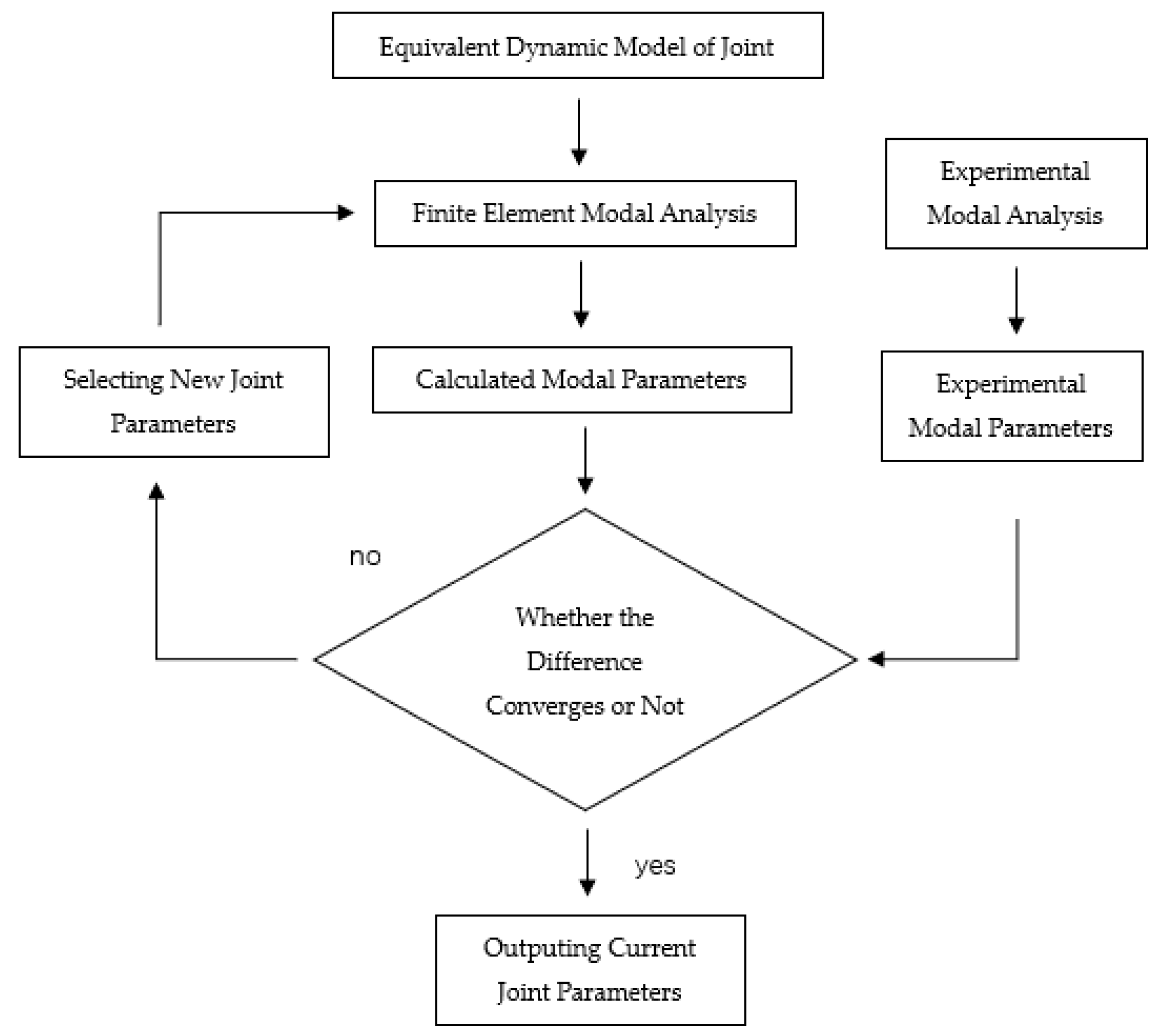
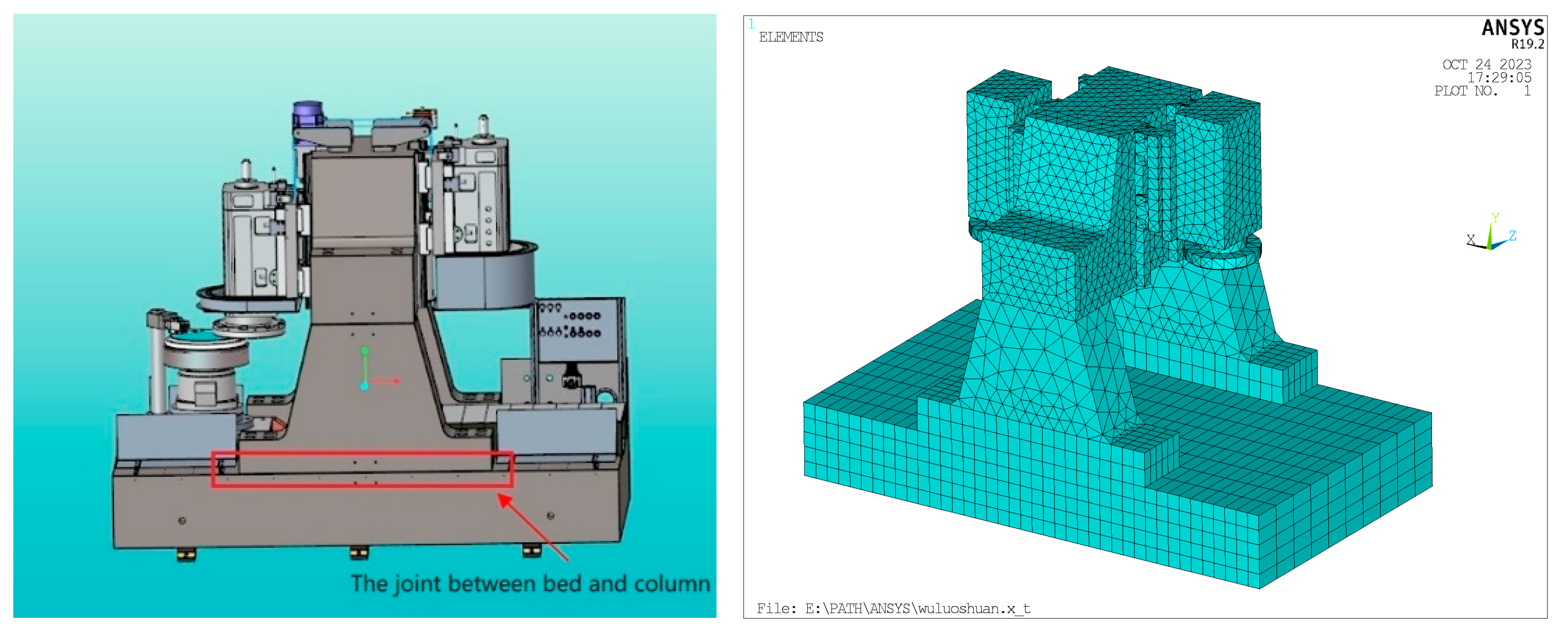
2.1. Principle of Joint Simulation Method Based on Matlab and Ansys

When the object is subjected to a resonant excitation force F, the differential equation of vibration of the system is given as

$$m\ddot{x}+c\dot{x}+kx=F$$

(1)

The Laplace transform of both sides of Equation (1) leads to Equation (2):

$$\left(m{s}^2+cs+k\right)x\left(s\right)=F\left(s\right)$$

(2)

Therefore, the transfer function H(s) is expressed as

$$H\left(s\right)=\frac{x\left(s\right)}{F\left(s\right)}=\frac{1}{m{s}^2+cs+k}$$

(3)

Let s = jω; the Laplace transform is transformed into the Fourier transform, and the transfer function H(s) is transformed into the frequency response function H(ω) in the frequency domain.

$$H\left(\omega \right)=\frac{1}{-{\omega }^{2}m+j\omega c+k}$$

(4)

The frequency response function responds to the relationship between the steady-state output and input of the system for a given frequency, and the natural frequency ω of the system can be identified according to the frequency response function, as shown in Equation (5):

$$k=m{\omega }^2$$

(5)

As long as the stiffness k is known, the natural frequency ω can be obtained; thus, the joint simulation in Matlab and Ansys is proposed to identify joint stiffness. The spring element of Ansys (combin14) is applied to simulate the joint, and the stiffness k is selected randomly by the genetic algorithm of Matlab. The stiffness value is substituted into the spring element, and then calculated natural frequencies are obtained by modal analysis. Experimental natural frequencies are obtained by modal test. Comparing the calculated natural frequency f_c with the experimental natural frequency f_test, when the difference converges, the values of the stiffness at this time are joint stiffnesses. The identification method of joint stiffness is shown in Figure 2.

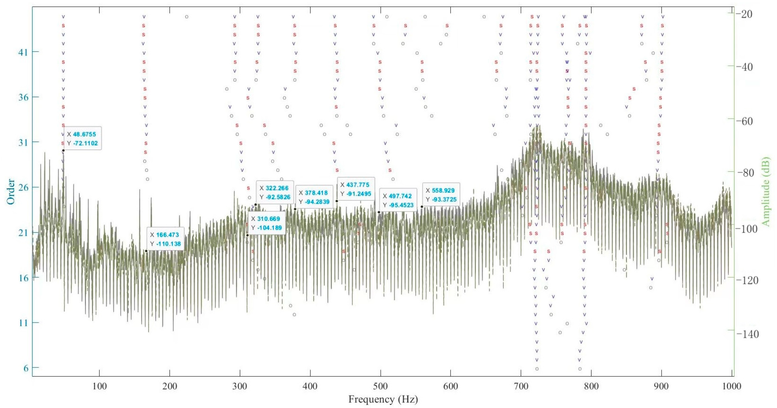
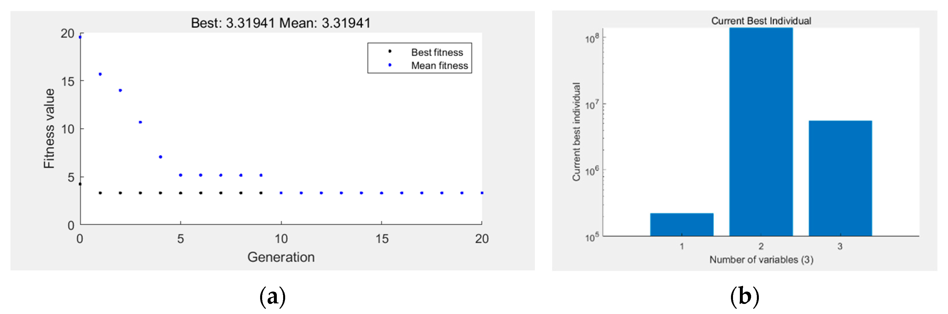
2.2. Method Verification

The method is applied to identify the stiffness of the bed–column joint of the precision grinding machine, as shown in Figure 3.

The accelerometer is fixed on the column, and the vibration signal of the joint is obtained by rotating the spindle. The signal is first processed by Kalman filtering, and then the natural frequencies of the joint are obtained by the least squares complex frequency domain method, as shown in Figure 4. Taking the first three orders as experimental natural frequencies from Figure 4, the first-order, second-order, and third-order experimental natural frequencies are 48.7 Hz, 166.5 Hz, and 310.7 Hz, respectively.

The joint stiffness is used as the design variable, and the calculated natural frequency fc is used as the state variable. Equation (6) is the objective function, and the stiffness value is outputted when the y-value converges.

$$y=\sqrt{w_1{\left(f_{1c}-f_{1test}\right)}^2+w_2{\left(f_{2c}-f_{2test}\right)}^2+\mathrm{\dots }+w_n{\left(f_{nc}-f_{ntest}\right)}^2}$$

(6)

where ${\omega }_1$ is the weights (${0<\omega }_1<1$), $f_{1c}$ is the calculated natural frequency, and $f_{1test}$ is the experimental natural frequency.

The joint simulation process and simulation results are shown in Figure 5. Figure 5a indicates the relationship between the best fitness value and the mean fitness value in each generation. The best fitness is the minimum y value in the current generation, and the mean fitness is the mean value of y in the current generation. As can be seen from Figure 5a, the difference between the best fitness and the mean fitness gradually decreases, and the two values are equal in the tenth generation, at which time the y value converges, and the corresponding solution is the optimal solution. The optimal solution is shown in Figure 5b, and from Figure 5b, the identified stiffnesses are 1.68 × 10¹⁰ N/m in the normal direction and 2.46 × 10⁷ N/m and 6.16 × 10⁸ N/m in the tangential direction, respectively.

The identified stiffness parameters are substituted into the model for modal analysis to obtain the natural frequencies considering the joint. The glue operation in Ansys is applied to bond the two objects together to obtain the natural frequencies without considering the joint. By comparing natural frequencies considering the joint with natural frequencies without considering the joint, as shown in

Table 1. Natural frequency comparison.

	First Order (Hz)	Second Order (Hz)	Third Order (Hz)
Experiment	48.7	166.5	310.7
Considering joint	48.8	165.8	313.6
Without considering joint	402.1	842.5	1068.9

, it can be seen that the simulation considering the influence of the joint is closer to the experimental results, which verifies the accuracy of the method of identifying the joint stiffness. It can also be seen that the presence of the joint reduces the overall natural frequencies of the structure significantly, proving that the presence of the joint needs to be taken into account when analyzing machine tools.

The method of identifying the stiffness of the joint is based on experimental natural frequencies, and the accuracy of natural frequencies obtained from the modal experiment directly determines the accuracy of the method. However, the modal experiment is generally carried out on the machine tool. Although sensors are placed on the joint to be measured, the response will still be affected by the influence of other components. The response obtained by the sensor is the result of the vibration of the joint to be measured and other components. Natural frequencies obtained by the modal experiment will have errors, which will affect the accuracy of the stiffness identified by the joint simulation method. Therefore, this paper corrects the fractal model of the normal stiffness of the joint so as to make the theoretical model better characterize the actual surface.

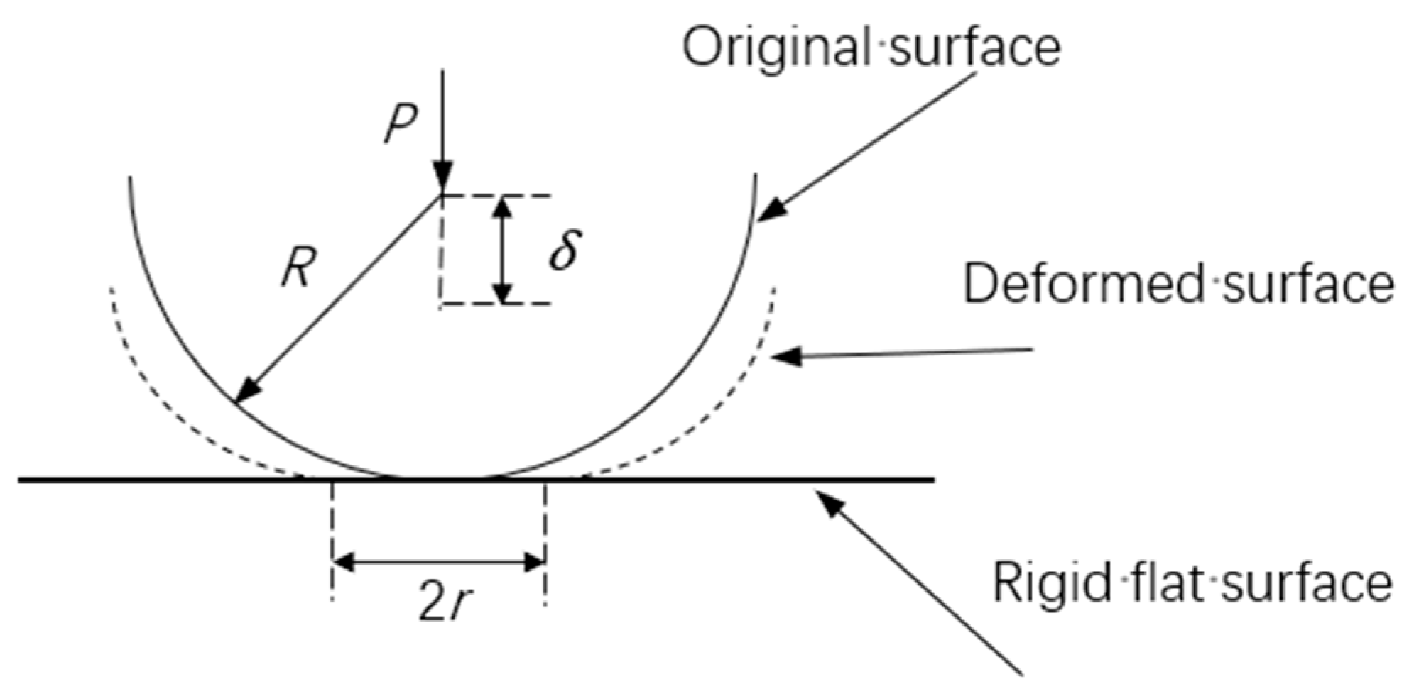
3. Modification of the Normal Stiffness Fractal Model for Joint

Majumdar and Bhushan proposed a contact fractal model (M-B fractal model) based on fractal geometry. The M-B fractal model simplifies the contact between rough surfaces to the contact between a rough surface and the ideal rigid plane, as shown in Figure 6, and this rough surface has fractal properties [3]. In the schematic diagram, P is the load between the contact points, R is the radius of curvature of the tip of asperity, δ is the deformation, and r is the radius of the contact area.

Greenwood found experimentally that the deformation of asperity changed from elasticity to plasticity when the deformation δ is greater than the critical deformation δ_c, in which case the critical deformation is given as [2]

$${\delta }_c=\frac{{\left(\pi k\varphi \right)}^2}{2}R$$

(7)

k and $\varphi$ satisfy the following relations, respectively:

$$k=\frac{H}{{\sigma }_y}$$

(8)

$$\varphi =\frac{{\sigma }_y}{E}$$

(9)

where H denotes the hardness of the softer material in Brinell units, σ_y denotes the yield strength of the softer material, and E denotes the composite Young’s modulus of the contact material, which is defined by the elastic modulus and Poisson’s ratio of the two contacting materials, as shown in Equation (10):

$$E=\frac{1-{\nu }_1{}^2}{E_1}+\frac{1-{\nu }_2{}^2}{E_2}$$

(10)

The surface contour line of the joint can be determined by the W-M function, as shown in Equation (11) [3]:

$$Z(x)=G^{\left(D-1\right)}\cdot l^{\left(2-D\right)}\cdot \cos \frac{\pi x}{l}$$

(11)

where D is the fractal dimension (1 < D < 2), G is the fractal roughness parameter, and l denotes the length scale.

From Equation (11), the radius of curvature of the tip of asperity can be derived as

$$R=\left|\frac{1}{{\left|\frac{d^{2}z}{d{x}^2}\right|}_{x=0}}\right|=\frac{a^{\frac{D}{2}}}{{\pi }^2{G}^{\left(D-1\right)}}$$

(12)

a is the contact area, as shown in Equation (13).

$$a=\pi r^2$$

(13)

The relationship between the contact area and the contact length is given as

$$l=a^{\frac{1}{2}}$$

(14)

From Equations (11) and (14), the deformation of asperity can be derived as

$$\delta =G^{\left(D-1\right)}\cdot l^{\left(2-D\right)}=G^{\left(D-1\right)}\cdot a^{\frac{2-D}{2}}$$

(15)

When the deformation δ of asperity is smaller than the critical deformation δ_c, it is in the elastic deformation stage. According to the Hertz contact theory, the relationship between load and deformation of a single asperity in the elastic deformation stage is given as follows (in this paper, P denotes the load of the individual asperity, and P′ denotes the total load of the joint):

$$P=\frac{4}{3}E{R}^{\frac{1}{2}}{\delta }^{\frac{4}{3}}$$

(16)

It was found that asperity interaction significantly affected the mean surface spacing and asperity load redistribution, and the deformation of asperity had to take into account the combined effect of load and asperity interaction. The actual deformation of asperity is given as [7]

$$\delta ={\delta }^{\prime }-{\delta }^{″}={\left(\frac{9P^2}{16E^{2}R}\right)}^{\frac{1}{3}}$$

(17)

where δ′ is the deformation due to normal loads, and δ″ is the additional deformation generated by asperity interaction.

Substituting Equation (17) into Equation (16), the relationship between the load and deformation of a single asperity in the elastic deformation stage can be derived as

$$P=\frac{E{a}^{\frac{3}{2}}}{\pi R}\left(1-\frac{3}{16}\pi \right)$$

(18)

When the deformation δ of asperity is larger than the critical deformation δ_c, it is not completely in the plastic stage but also exists in the elastic–plastic stage, and the elastic–plastic deformation range is δ_c ≤ δ ≤ 110 δ_c. The elastic–plastic deformation is divided into two stages. When δ_c ≤ δ ≤ 6 δ_c, yielding occurs underneath the contact surface, and the yielding region increases with the increase in load. When δ = 6 δ_c, yielding occurs on the entire contact surface, at which time the average pressure on the contact surface is smaller than the material hardness until δ = 110 δ_c, and the average pressure on the contact surface is equal to the material hardness. When δ > 110 δ_c, asperity enters the fully plastic deformation stage. When δ_c ≤ δ ≤ 6 δ_c, the relationship between contact load and deformation at the contact point is given as [18]

$$P_1=P_c\cdot 1.03\cdot {\left(\frac{\delta }{{\delta }_c}\right)}^{1.425}$$

(19)

where P_c is the critical load. P_c is given as

$$P_c=\frac{4}{3}E{R}^{\frac{1}{2}}{\delta }_c{}^{\frac{4}{3}}$$

(20)

When 6 δ_c <δ ≤ 110 δ_c, the relationship between contact load and deformation at the contact point is given as [18]

$$P_2=P_c\cdot 1.4\cdot {\left(\frac{\delta }{{\delta }_c}\right)}^{1.236}$$

(21)

When the deformation δ of asperity is larger than 110 δ_c, it is in the fully plastic stage, and the relationship between contact area and load at the plastic contact point is given as

$$P_p=H\cdot a$$

(22)

It has been shown that the effect of the asperity interaction can be largely counteracted by the plastic deformation of asperity [19], so the influence of the interaction on the deformation of asperity in the elastic–plastic and fully plastic stage is not considered in this paper.

3.1. Total Normal Load of Joint

When δ = δ_c, the contact area is the critical contact area a_c

$$a_c=\frac{G^2}{{\left(\frac{k\varphi }{2}\right)}^{\frac{2}{D-1}}}$$

(23)

From $\frac{{\delta }_c}{\delta }={\left(\frac{a}{a_c}\right)}^{(D-1)}$, it can be seen that if the contact area of asperity a < a_c, i.e., the deformation δ > δ_c, the contact deformation occurs as elastic–plastic deformation or plastic deformation. If ${\frac{1}{6}}^{\frac{1}{D-1}}{a}_c\le a\le a_c$, the deformation occurs in the elastic–plastic first stage. If ${{\frac{1}{110}}^{\frac{1}{D-1}}{a}_c\le a}_c\le {\frac{1}{6}}^{\frac{1}{D-1}}{a}_c$, the deformation occurs in the elastic–plastic second stage. If $0\le a\le {\frac{1}{110}}^{\frac{1}{D-1}}{a}_c$, the deformation is completely plastic. If the contact area of asperity a > a_c, which means that the deformation δ < δ_c, the contact deformation is elastic deformation.

In the elastic stage, the total load P_e′ can be derived as

$$P_e{}^{\prime }={\displaystyle {\int }_{a_c}^{a_l}Pn\left(a\right)da}=\frac{\left(16-3\pi \right)\left(a_l{}^{\frac{3}{2}}-a_c{}^{\frac{3-D}{2}}{a}_l{}^{\frac{D}{2}}\right)}{16R\pi \left(3-D\right)}$$

(24)

where a_l is the maximum contact area of individual asperity, and n(a) is area distribution density. n(a) is given as [1]

$$n\left(a\right)=\frac{D}{2}\cdot \frac{a_l{}^{\frac{D}{2}}}{a^{\left(\frac{D}{2}+1\right)}}$$

(25)

In the elastic–plastic stage, the total load in the elastic–plastic first stage can be derived as

$$\begin{array}{ll}{P}_{e1}{}^{\prime }& ={\displaystyle {\int }_{{\frac{1}{6}}^{\frac{1}{D-1}}{a}_c}^{a_c}{P}_{1}n\left(a\right)da}\\ & =\frac{24.7543\cdot D{E}^{0.85}{G}^{0.85\left(D-1\right)}{H}^{0.15}{a}_l{}^{0.5D}{k}^{0.15}\left(6^{\frac{\left(0.925D-1.425\right)a_c}{D-1}}-a_c{}^{\left(1.425-0.925D\right)}\right)}{\left(37D-57\right)\pi }\end{array}$$

(26)

The total load in the elastic–plastic second stage can be derived as

$$\begin{array}{ll}{P}_{e2}{}^{\prime }& ={\displaystyle {\int }_{{\frac{1}{110}}^{\frac{1}{D-1}}{a}_c}^{{\frac{1}{6}}^{\frac{1}{D-1}}{a}_c}{P}_{2}n\left(a\right)da}\\ & =\frac{161.8203\cdot D{E}^{0.472}{G}^{0.8472\left(D-1\right)}{H}^{0.528}{a}_l{}^{0.5D}{k}^{0.528}\left(6^{\frac{\left(0.736D-1.236\right)a_c}{D-1}}-{110}^{\frac{\left(0.736D-1.236\right)a_c}{D-1}}\right)}{\left(309-184D\right)\pi }\end{array}$$

(27)

The total load in the fully plastic stage can be derived as

$${P^{\prime }}_l={\displaystyle {\int }_0^{{\frac{1}{110}}^{\frac{1}{D-1}}{a}_c}{P}_{p}n\left(a\right)da}=\frac{{110}^{\frac{a_c\left(D-2\right)}{2\left(D-1\right)}}DH{a}_l{}^{\frac{D}{2}}}{D-2}$$

(28)

Therefore, the total normal load P of the joint is given as

$$P^{\prime }=P_e{}^{\prime }+P_{e1}{}^{\prime }+P_{e2}{}^{\prime }+P_l{}^{\prime }$$

(29)

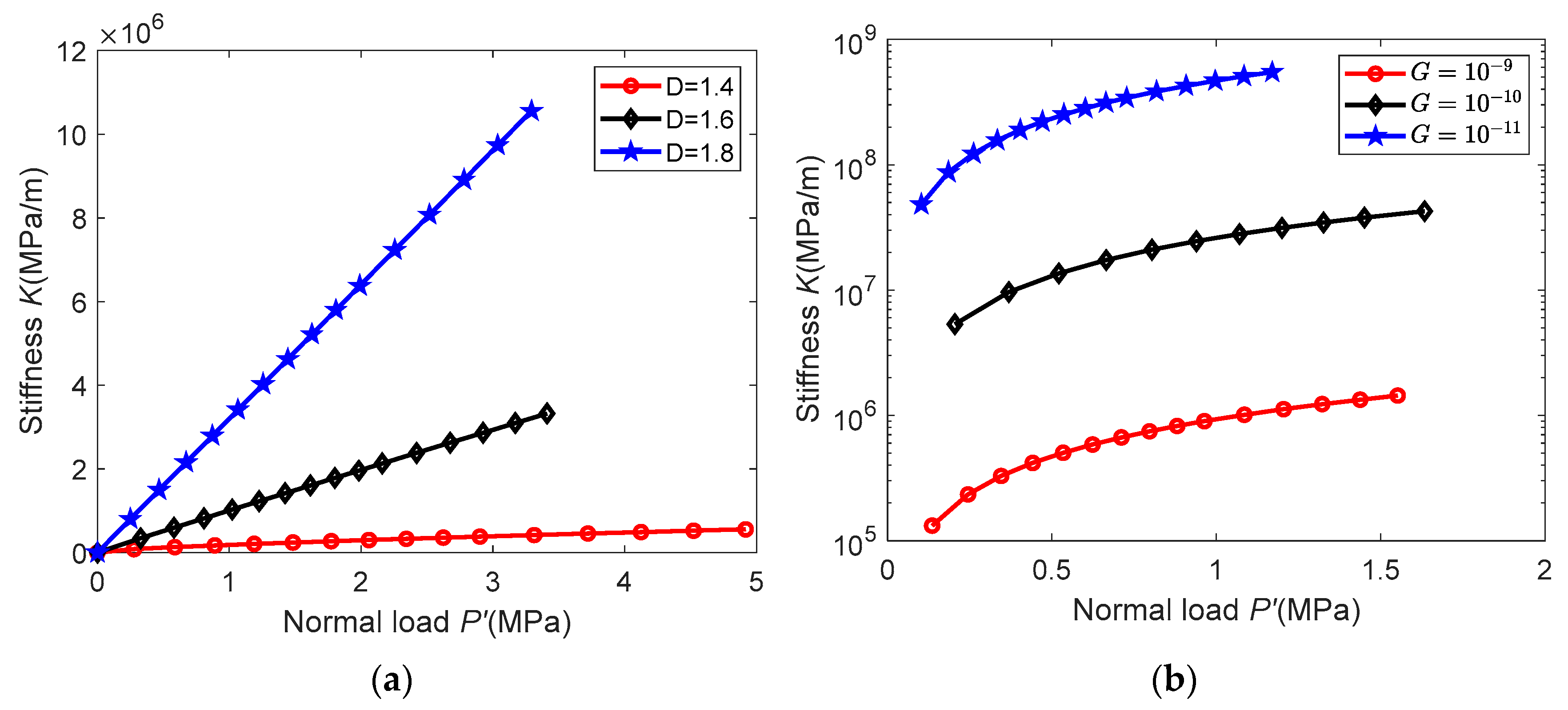
3.2. Total Normal Stiffness of Joint

The stiffness k_e of the individual asperity in the elastic stage can be derived as follows (in this paper, lowercase k denotes the stiffness of the individual asperity, and uppercase K denotes the total stiffness of the joint):

$$k_e=\frac{dP}{d\delta }=2E\sqrt{\frac{3a}{16}}$$

(30)

The total normal stiffness K_e in the elastic stage can be expressed as

$$K_e={\displaystyle {\int }_{a_c}^{a_l}kn\left(a\right)da}=\frac{\sqrt{3}ED{a}_l{}^{\frac{D}{2}}}{2\left(1-D\right)}\left(a_l{}^{\frac{1-D}{2}}-a_c{}^{\frac{1-D}{2}}\right)$$

(31)

During the elastic–plastic stage, the stiffness of the individual asperity in the elastic–plastic first stage can be derived as

$$k_{e1}{}^{\prime }=\frac{d{P}_1}{d\delta }=\frac{2}{3}KH\frac{1.03\cdot 1.425}{0.93}a{\left(\frac{\delta }{{\delta }_c}\right)}^{-0.711}\frac{1}{{\delta }_c}$$

(32)

The total stiffness K₁ in the elastic–plastic first stage can be expressed as

$$\begin{array}{ll}{K}_1& ={\displaystyle {\int }_{{\frac{1}{6}}^{\frac{1}{D-1}}{a}_c}^{a_c}{k}_{e1}{}^{\prime }n\left(a\right)da}\\ & =\frac{17.6375\cdot 2^{0.85}\cdot 3^{0.075}\cdot DE{G}^{0.15\left(1-D\right)}{H}^{0.15}{a}_l{}^{0.5D}\left(6^{\frac{\left(0.425D-0.5\right)a_c}{D-1}}-a_c{}^{\left(0.5-0.425D\right)}\right)}{\left(17D-20\right)\pi }\end{array}$$

(33)

The stiffness of the individual asperity in the elastic–plastic second stage can be derived as

$$k_{e2}{}^{\prime }=\frac{d{P}_2}{d\delta }=\frac{2}{3}KH\frac{1.4\cdot 1.236}{0.94}a{\left(\frac{\delta }{{\delta }_c}\right)}^{-0.236}\frac{1}{{\delta }_c}$$

(34)

The total stiffness K₂ in the elastic–plastic second stage can be expressed as

$$\begin{array}{ll}{K}_2& ={\displaystyle {\int }_{{\frac{1}{110}}^{\frac{1}{D-1}}{a}_c}^{{\frac{1}{6}}^{\frac{1}{D-1}}{a}_c}{k}_{e2}{}^{\prime }n\left(a\right)da}\\ & =\frac{161.8203\cdot 2^{0.472}\cdot 3^{0.264}DE{G}^{0.528(1-D)}{H}^{0.528}{a}_l{}^{0.5D}\left(6^{\frac{\left(0.236D-0.5\right)a_c}{D-1}}-{110}^{\frac{\left(0.236D-0.5\right)a_c}{D-1}}\right)}{\left(125-59D\right)\pi }\end{array}$$

(35)

Therefore, the total normal stiffness of joint K is given as

$$K=K_e+K_1+K_2$$

(36)

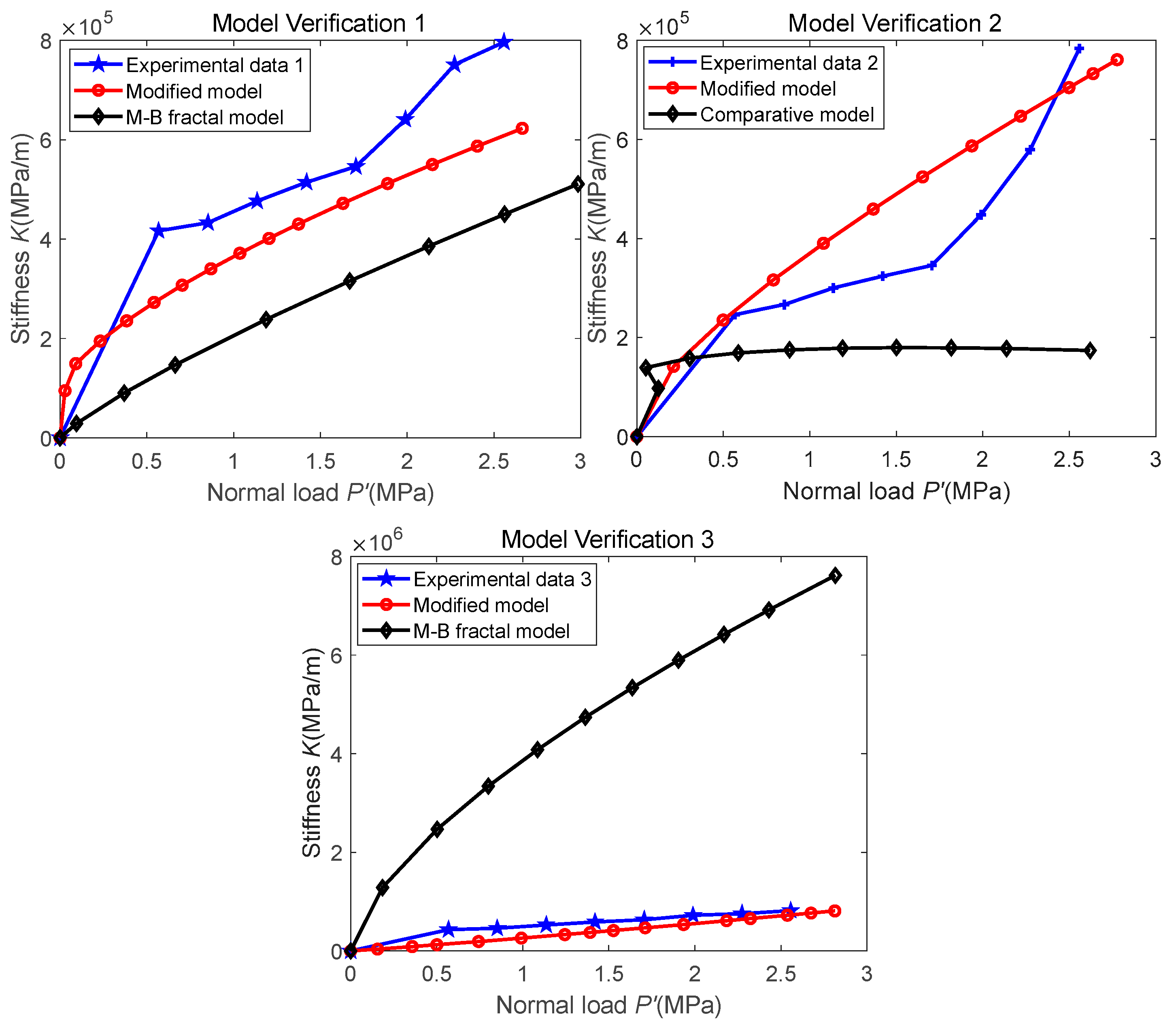
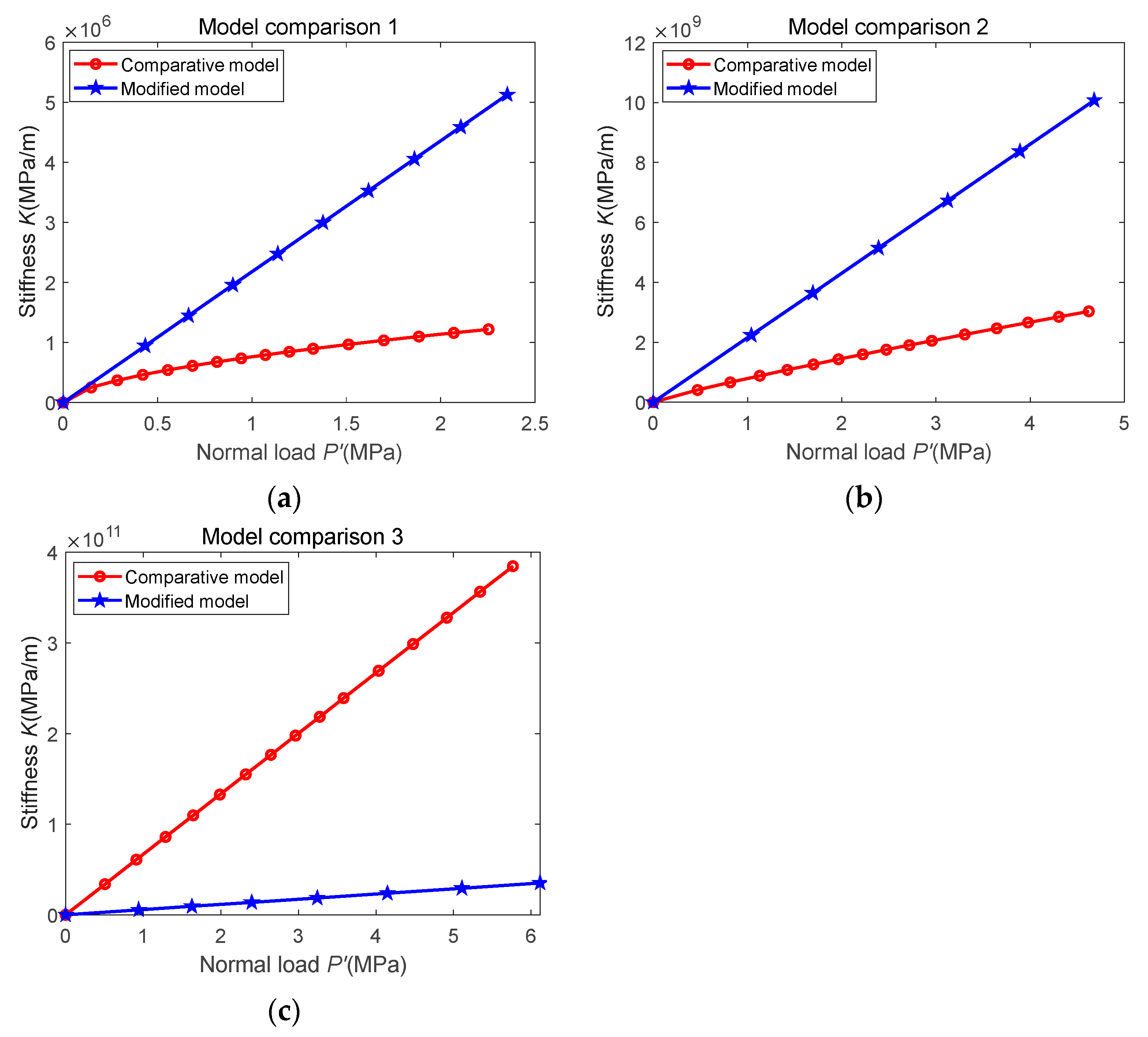
3.3. Numerical Simulation and Model Verification

Numerical simulation of the modified model is carried out, and the simulation results are shown in Figure 7. It can be seen that the normal stiffness of the joint increases with the increase in normal load, increases with the increase in D, and decreases with the increase in G. The larger the normal load is, the more asperity is in contact with each other on the joint. Therefore, the proportion of elastic deformation increases, and the ability to resist deformation increases, i.e., the stiffness increases. The larger D is, the smaller G is, and the smoother the joint is. There is more asperity squeezing each other, and hence, the stiffness increases.

To further verify the feasibility of the modified model, the experimental data from reference [7] are used to verify the modified model. Compared with the MB model, as shown in Figure 8, it can be seen that the modified model is closer to the experimental data than the MB model, which verifies the feasibility of the modified model.

4. Three-Dimensional Fractal Model

The modified normal stiffness fractal model for the joint is closer to reality after considering the elastic–plastic deformation and asperity interaction. Since the W-M function is a two-dimensional function, the fractal model is only a two-dimensional model, which does not match the actual three-dimensional morphology of the surface. Based on this, the two-dimensional model is extended into a three-dimensional model, and the friction factor is included. Therefore, the normal stiffness fractal model is further modified. Yan et al. improved the traditional W-M function to obtain a three-dimensional fractal surface, and the modified W-M function is given as follows [20]:

$$\begin{array}{ll}Z\left(x,y\right)& =L{\left(\frac{G}{L}\right)}^{D-2}{\left(\frac{\ln \gamma }{M}\right)}^{\frac{1}{2}}\\ & \cdot {\displaystyle \sum _{m=1}^M{\displaystyle \sum _{n=0}^{n_{\max }}{\gamma }^{\left(D-3\right)n}\cdot \left\{\cos \phi -\cos \left[\frac{2\pi {\gamma }^n{\left(x^2+y^2\right)}^{\frac{1}{2}}}{L}\cdot \cos \left({\tan }^{-1}(\frac{y}{x})-\frac{\pi m}{M}\right)+\phi \right]\right\}}}\end{array}$$

(37)

where D is the fractal dimension (2 < D < 3), G is the fractal roughness, γ is the scale factor, L is the sampling length, M is the number of surface ridges, φ is the random phase, and n is the frequency index.

Simulation of the 3D W-M function, as shown in Figure 9, reveals that the surface is smoother as D increases, which is consistent with the known conclusions, indicating that the actual surface topography can be better simulated with the 3D fractal model.

From Equation (37), the deformation of asperity can be derived as

$$\delta =2^{\frac{11-3D}{2}}{G}^{\left(D-2\right)}{\left(\ln \gamma \right)}^{0.5}{\pi }^{\frac{D-3}{2}}{a}^{\frac{3-D}{2}}$$

(38)

From Equation (38), the equivalent radius of curvature of asperity can be derived as

$$R=\frac{2^{\frac{3D-11}{2}}{\pi }^{\frac{1-D}{2}}{G}^{2-D}{a}^{\frac{D-1}{2}}}{{\left(\ln \gamma \right)}^{0.5}}$$

(39)

Considering the friction factor, the critical deformation of asperity is given as [21]

$${\delta }_c={\left(\frac{33\pi k_{\mu }\varphi }{40}\right)}^{2}R$$

(40)

where $k_{\mu }$ is the friction correction factor.

When δ = δ_c, the contact area a is the critical contact area a_c, which can be calculated from Equations (38)–(40):

$$a_c=2^{\frac{3D-11}{2-D}}{\left(\frac{33\pi k_{\mu }\varphi }{40}\right)}^{\frac{2}{2-D}}{\pi }^{\frac{4-D}{2-D}}{\left(\ln \gamma \right)}^{\frac{1}{D-2}}{G}^2$$

(41)

4.1. Total Load and Total Stiffness

From Equations (19), (39) and (40), the total load in the elastic–plastic first stage can be derived as

$$\begin{array}{ll}{P}_{e1}{}^{\prime }& ={\displaystyle {\int }_{{\frac{1}{6}}^{\frac{1}{D-1}}{a}_c}^{a_c}{P}_{1}n\left(a\right)da}\\ & =15.7636\cdot 2^{0.225-1.275D}DE{G}^{0.85D-1.7}{a}_l{}^{0.5D}{\varphi }^{0.15}{k}_{\mu }{}^{0.15}{\pi }^{0.425D-1.7}{\left(\ln \gamma \right)}^{0.425}\\ & \cdot \frac{6^{\frac{\left(0.925D-1.85\right)a_c}{D-1}}-a_c{}^{\left(1.85-0.925D\right)}}{D-2}\end{array}$$

(42)

From Equations (21), (39) and (40), the total load in the elastic–plastic second stage can be derived as

$$\begin{array}{ll}{P}_{e2}{}^{\prime }& ={\displaystyle {\int }_{{\frac{1}{110}}^{\frac{1}{D-1}}{a}_c}^{{\frac{1}{6}}^{\frac{1}{D-1}}{a}_c}{P}_{2}n\left(a\right)da}\\ & =6.8692\cdot 2^{0.012-0.708D}DE{G}^{0.472D-0.944}{a}_l{}^{0.5D}{\varphi }^{0.528}{k}_{\mu }{}^{0.528}{\pi }^{0.236D-0.944}{\left(\ln \gamma \right)}^{0.236}\\ & \cdot \frac{{110}^{\frac{\left(0.736D-1.472\right)a_c}{D-1}}-6^{{}^{\frac{\left(0.736D-1.472\right)a_c}{D-1}}}}{D-2}\end{array}$$

(43)

The total normal load P′ of the joint is given as

$$P^{\prime }=P_e{}^{\prime }+P_{e1}{}^{\prime }+P_{e2}{}^{\prime }+P_l{}^{\prime }$$

From Equations (32), (39) and (40), the total stiffness in the elastic–plastic first stage can be derived as

$$\begin{array}{ll}{K}_1& ={\displaystyle {\int }_{{\frac{1}{6}}^{\frac{1}{D-1}}{a}_c}^{a_c}{k}_{e1}{}^{\prime }n\left(a\right)da}\\ & =12.9865\cdot 2^{0.725+0.225D}DE{G}^{0.3-0.15D}{a}_l{}^{0.5D}{\varphi }^{0.15}{k}_{\mu }{}^{0.15}\\ & \cdot \frac{6^{\frac{\left(0.175D-0.35\right)a_c}{D-1}}-a_c{}^{\left(0.35-0.175D\right)}}{\left(17D-14\right){\pi }^{0.075D+0.2}{\left(\ln \gamma \right)}^{0.075}}\end{array}$$

(44)

From Equations (34), (39) and (40), the total stiffness in the elastic–plastic second stage can be derived as

$$\begin{array}{ll}{K}_2& ={\displaystyle {\int }_{{\frac{1}{110}}^{\frac{1}{D-1}}{a}_c}^{{\frac{1}{6}}^{\frac{1}{D-1}}{a}_c}{k}_{e2}{}^{\prime }n\left(a\right)da}\\ & =24.4098\cdot 2^{0.512+0.792D}DE{G}^{1.056-0.528D}{a}_l{}^{0.5D}{\varphi }^{0.528}{k}_{\mu }{}^{0.528}{\pi }^{0.556-0.264D}\\ & \cdot \frac{{110}^{\frac{\left(0.236D+0.028\right)a_c}{D-1}}-6^{\frac{\left(0.236D+0.028\right)a_c}{D-1}}}{D-2}\end{array}$$

(45)

The total normal stiffness of joint K is given as

$$K=K_e+K_1+K_2$$

4.2. Numerical Simulation

Numerical simulations are conducted for the 3D-modified model. The relationship of normal stiffness with normal load, D and G, is shown in Figure 10. It can be seen that the normal stiffness increases with the increase in normal load and D and increases with the decrease in G, which is consistent with the existing conclusions. Numerical simulation initially verifies the rationality of the modified model.

The modified model is compared with the three-dimensional normal stiffness fractal model of joint derived from the reference [22], as shown in Figure 11. It can be seen that the modified model has the same trend of change as the compared model, which further verifies the reasonableness of the modified model.

To prove the accuracy of the 3D normal stiffness fractal model, the model is compared with the 2D fractal model modified in Chapter 3, as shown in Figure 12. The 3D fractal dimension D is obtained by adding 1 to the fractal dimension D in the 2D fractal model. The 3D fractal model is larger than the 2D fractal model in numerical values. Combined with Figure 8, it can be seen that the 3D fractal model is closer to the experimental data, so the modified 3D fractal model is more accurate.

5. Conclusions

This paper proposes a joint simulation in Matlab and Ansys to identify the joint stiffness. The method is applied to identify the joint between the bed and column of a precision grinding machine. In order to further study the joint contact, the contact between asperity is studied from a microscopic point of view. The theoretical model based on fractal geometry is amended so that the theoretical model can more accurately characterize the actual surface contact. The conclusions obtained are as follows.

• The method based on joint simulation in Matlab and Ansys can identify the joint stiffness quickly and accurately;
• Simulation of the dynamic performance of a machine tool considering the joint is closer to the experimental data than without considering the joint;
• The existence of the joint reduces the overall natural frequencies of the machine tool;
• The 2D fractal model is more accurate after considering the asperity interaction and elastic–plastic deformation. The normal stiffness increases with the increase in normal load and D and increases with the decrease in G;
• The calculated stiffness of the 3D fractal model is greater than that of the 2D fractal model, and the 3D fractal model can more accurately characterize the actual surface.

References

1. Zhang, X.L. Dynamic Characterization and Applications for Machine Joint Interfaces; Science and Technology of China Press: Beijing, China, 2002. [Google Scholar]
2. Greenwood, J.A.; Williamson, J.B.P. Contact of nominally flat surfaces. Proc. R. Soc. Lond. Ser. A Math. Phys. Sci. 1966, 295, 300–319. [Google Scholar]
3. Majumdar, A.; Bhushan, B. Fractal model of elastic-plastic contact between rough surfaces. J. Tribol. 1991, 113, 1–11. [Google Scholar] [CrossRef]
4. Kogut, L.; Etsion, I. A finite element based elastic-plastic model for the contact of rough surfaces. Tribol. Trans. 2003, 46, 383–390. [Google Scholar] [CrossRef]
5. Chang, W.R.; Etsion, I.; Bogy, D.B. An elastic-plastic model for the contact of rough surfaces. J. Tribol. 1987, 109, 257–263. [Google Scholar] [CrossRef]
6. Ciavarella, M.; Greenwood, J.A.; Paggi, M. Inclusion of “interaction” in the Greenwood and Williamson contact theory. Wear 2008, 265, 729–734. [Google Scholar] [CrossRef]
7. Wang, R.; Zhu, L.; Zhu, C. Research on fractal model of normal contact stiffness for mechanical joint considering asperity interaction. Int. J. Mech. Sci. 2017, 134, 357–369. [Google Scholar] [CrossRef]
8. Zhu, L.; Chen, J.; Zhang, Z.; Hong, J. Normal contact stiffness model considering 3D surface topography and actual contact status. Mech. Sci. 2021, 12, 41–50. [Google Scholar] [CrossRef]
9. Xue, P.; Zhu, C.; Wang, R.; Zhu, L. Research on dynamic characteristics of oil-bearing joint surface in slide guides. Mech. Based Des. Struct. Mach. 2022, 50, 1893–1913. [Google Scholar] [CrossRef]
10. Jiang, K.; Liu, Z.; Yang, C.; Zhang, C.; Tian, Y.; Zhang, T. Effects of the joint surface considering asperity interaction on the bolted joint performance in the bolt tightening process. Tribol. Int. 2022, 167, 107408. [Google Scholar] [CrossRef]
11. Li, L.; Wang, J.; Shi, X.; Ma, S.; Cai, A. Contact stiffness model of joint surface considering continuous smooth characteristics and asperity interaction. Tribol. Lett. 2021, 69, 1–12. [Google Scholar] [CrossRef]
12. Mottershead, J.E.; Stanway, R. Identification of structural vibration parameters by using a frequency domain filter. J. Sound Vib. 1986, 109, 495–506. [Google Scholar] [CrossRef]
13. Tsai, J.S.; Chou, Y.F. The identification of dynamic characteristics of a single bolt joint. J. Sound Vib. 1988, 125, 487–502. [Google Scholar] [CrossRef]
14. Syed Asif, S.A.; Wahl, K.J.; Colton, R.J.; Warren, O.L. Quantitative imaging of nanoscale mechanical properties using hybrid nanoindentation and force modulation. J. Appl. Phys. 2001, 90, 1192–1200. [Google Scholar] [CrossRef]
15. Kartal, M.E.; Mulvihill, D.M.; Nowell, D.; Hills, D.A. Determination of the frictional properties of titanium and nickel alloys using the digital image correlation method. Exp. Mech. 2011, 51, 359–371. [Google Scholar] [CrossRef]
16. Mulvihill, D.M.; Brunskill, H.; Kartal, M.E.; Dwyer-Joyce, R.S.; Nowell, D. A comparison of contact stiffness measurements obtained by the digital image correlation and ultrasound techniques. Exp. Mech. 2013, 53, 1245–1263. [Google Scholar] [CrossRef]
17. Jamia, N.; Jalali, H.; Taghipour, J.; Friswell, M.I.; Khodaparast, H.H. An equivalent model of a nonlinear bolted flange joint. Mech. Syst. Signal Process. 2021, 153, 107507. [Google Scholar] [CrossRef]
18. Kogut, L.; Etsion, I. Elastic-plastic contact analysis of a sphere and a rigid flat. J. Appl. Mech. 2002, 69, 657–662. [Google Scholar] [CrossRef]
19. Zhao, Y.; Chang, L. A model of asperity interactions in elastic-plastic contact of rough surfaces. J. Trib. 2001, 123, 857–864. [Google Scholar] [CrossRef]
20. Yan, W.; Komvopoulos, K. Contact analysis of elastic-plastic fractal surfaces. J. Appl. Phys. 1998, 84, 3617–3624. [Google Scholar] [CrossRef]
21. Li, X.P.; Zhao, G.H.; Liang, Y.M. Fractal model and simulation of normal contact stiffness between two cylinders’ joint surfaces. Trans. Chin. Soc. Agric. Mach. 2013, 44, 277–281. [Google Scholar]
22. Li, X.P.; Wang, X.; Yun, H.M.; Gao, J.Z. Investgation into normal contact stiffness of fixed joint surface with three-dimensional fractal. J. S. China Univ. Technol. Nat. Sci. Ed. 2016, 1, 114–122. [Google Scholar]
Figure 1. Equivalent model of joint.
Applsci 13 11680 g001
Figure 2. Flowchart of the stiffness identification method.
Applsci 13 11680 g002
Figure 3. Joint interfaces to be measured.
Applsci 13 11680 g003
Figure 4. Experimental natural frequencies.
Applsci 13 11680 g004
Figure 5. Joint simulation. (a) Simulation process; (b) Simulation results.
Applsci 13 11680 g005
Figure 6. Joint contact model.
Applsci 13 11680 g006
Figure 7. Total normal stiffness along with P′, D, and G. (a) G = 10−9, E = 69.3 Gpa, ν = 0.25, and HB = 231; (b) D = 1.7, E = 69.3 Gpa, ν = 0.25, and HB = 231.
Applsci 13 11680 g007
Figure 8. Modal verification.
Applsci 13 11680 g008
Figure 9. Three-dimensional W-M function: L = 0.89, γ = 1.5, M = 2, and G = 1.36 ×   10 7 . (a) D = 2.1; (b) D = 2.5; (c) D = 2.8.
Applsci 13 11680 g009
Figure 10. Total normal stiffness along with P′, D, and G.
Applsci 13 11680 g010
Figure 11. Model comparison. G = 10 9 γ = 1.5 = 2.5 . (a) D = 2.1; (b) D = 2.4; (c) D = 2.7.
Applsci 13 11680 g011
Figure 12. Model comparison.
Applsci 13 11680 g012