Dual PID Adaptive Variable Impedance Constant Force Control for Grinding Robot

Abstract

High-precision and low-overshoot force control are important to guarantee the material removal rate and surface quality of robot grinding. However, traditional force control methods are subjected to positional disturbance, stiffness disturbance, contact process nonlinearity, and force-position coupling, leading to difficulties in robot constant force control. Therefore, how to achieve smooth, stable, and high-precision constant force control is an urgent problem. To address this problem, a dual PID adaptive variable impedance control is established (DPAVIC). Firstly, PD control is used to compensate for the force error, and PID is used to update the damping parameters to compensate for the disturbance. Secondly, a nonlinear tracking differentiator is used to smooth the desired force and reduce the contact force overshoot. Then, the stability, convergence, and effectiveness of the force control algorithm are verified via theoretical analysis, simulations, and experiments. The force tracking error and overshoot of a conventional impedance controller (CIC), adaptive variable impedance control (AVIC), and DPAVIC are analyzed. Finally, the algorithm is used in grinding experiments on a thin-walled workpiece. The force tracking error is controlled within ±0.2 N, and the surface roughness of the workpiece is improved to Ra 0.218 $\mathsf{\mu }$m.

1. Introduction

In the manufacturing process of molds, aircraft panels, sculptures, etc., grinding and polishing are used to reduce the surface roughness and improve the machining accuracy [1,2]. However, most grinding and polishing operations are still performed manually, resulting in low manufacturing efficiency, poor workpiece surface quality, and worker health problems [3,4]. The automatic grinding and polishing processes represented by computer numerical control machine tools (CNCs) and industrial robots have become the main solutions [5,6]. CNCs not only have excellent stiffness and high precision positioning, but can also concurrently control trajectory, pose, and force [7]. However, the grinding space of CNCs is small, they have poor flexibility, and the machine tools need to be designed individually for large-scale special-shaped surfaces, which limit the application [8]. Robots have the advantages of a large working range, high flexibility, and have gradually become a research hot-spot in the field of grinding and polishing.

Robot grinding is a typical constrained operation. According to Preston’s law, the amount of workpieces removed increases monotonically with the increase in grinding force, tool speed, and residence time, the most important of which is the control of the grinding force [9]. Therefore, controlling the robot end contact force is of great significance to improve the surface quality [10,11]. However, applying position-based industrial robots directly to grinding and polishing processes involving contact motion is not straightforward [2,12]. An accurate and smooth contact force control method is the key to realize high-quality automatic grinding and polishing of robots.

Robot end contact force control methods are mainly divided into passive force control [13,14] and active force control [15,16]. Passive force control is achieved through energy absorption or the storage of the auxiliary flexibility mechanism, and the robot is still in position control mode [17,18]. Typical force control devices mainly include voice coil motor actuators [19,20], parallel mechanism actuators [21,22], pneumatic actuators [23,24,25], mechanically flexible structures [26,27,28,29], force control joints [30], etc. Chen et al. [31] adopted a dual force sensor to decouple the dynamics between the macro robot, micro robot, and workpiece to achieve high-precision force control. However, passive force control requires the installation of an actuator at the robot end, which puts forward higher requirements for the design of the end actuator in the case of a limited end load of the robots. Therefore, active force control is more feasible.

Active force control is the use of designed control strategies to actively control force through the feedback of contact force information [32]. In the aspect of force control algorithms, the design of the force controller is the most important, and the common force control algorithms are impedance control [33,34] and hybrid position/force control [35,36]. For uncertain environments, that is, when the stiffness and position of the environment are unknown, it is difficult to obtain an accurate model, which makes it difficult to achieve high-precision force tracking. There are three main solutions: (1) Indirect adjustment of the reference trajectory: the basic method is to identify environmental information, including stiffness and position [37,38]. (2) Direct adjustment of the reference trajectory: the basic method is to update the reference trajectory with prior information [39,40]. However, this method ignores the dynamic physical characteristics of the robot and the environment and usually results in a large force tracking error. (3) Adaptive variable impedance control: this method adaptively adjusts the controller parameters according to force feedback information [41,42,43]. To improve the accuracy of force tracking, the researchers combined the adaptive algorithm with other force control methods to obtain better force control results [44]. Examples include fuzzy logic control [45], robust force control [46], optimal control [47], etc. Therefore, the key to establish a force tracking controller is to compensate for environmental disturbance, which is oriented to practical applications, and the control method should not be too complicated.

Force overshoot usually occurs when the robot end effector touches the workpiece. Although this problem only occurs in a short time, it will lead to poor system stability and low surface quality. Therefore, it is extremely important to ensure the stability of the system [15]. The nonlinear feedback control method is used to plan the trajectory and contact force simultaneously to reduce the force overshoot [48]. Roveda et al. [49] adopted an impedance shaping method to reduce the influence of force overshoot on system stability and achieve stable contact state transition. These methods usually require accurate estimates of the environmental position and stiffness, and this approach is difficult.

In this work, a dual PID adaptive impedance control method is proposed to achieve smooth, stable, and high-precision robot end contact force control. PD is used to compensate for the force error, and PID is used to update the damping parameters to compensate for the environmental uncertainty. A nonlinear tracking differentiator is used to reduce the impact of the transitional contact state. The interference term of the end 6-Dof force sensor is compensated using the least square method to ensure the accuracy of force control. The stability, convergence, and effectiveness of the force control algorithm are verified with theoretical analysis, simulations, and experiments. Furthermore, the thin-walled workpiece is used in a robot grinding experiment to verify the accuracy of force control.

The remainder of this paper is organized as follows: In Section 2, a nonlinear tracking differentiator is used to stabilize the contact transition state. In Section 3, a position-based dual PID adaptive impedance control method is established to compensate for the uncertainty of environment. In Section 4, the interference term of the 6-Dof force sensor is compensated for. The proposed method is verified in MATLAB/Simulink in Section 5. In Section 6, the effectiveness of the method is verified via force control and grinding experiments.

2. Modeling of Grinding System and Suppression of Contact Force Overshoot

A grinding robot system is established, as shown in Figure 1. A 7-Axis Franka Emika Panda robot is used; a Dynpick 6-Dof force sensor (Type: WEF-6A200-4-RC24, the force measurement range is ±200 N and the moment measurement range is ±4 Nm. Manufacturer: WACOH-TECH. City: Tokyo. Country: Japan.), an analog IO module (Type: NET6043-S, 8-Channel 0-10V analog input module with resolution of 16-Bit. Manufacturer: HKTECH. City: Zhengzhou. Country: China.) and a grinding tool are installed at the end of the robot.

As shown in Figure 2, with the robot and the workpiece set as a spring-damp-mass system, the contact process between the robot and the workpiece can be divided into three stages [50]. Figure 2a shows that the robot does not have contact with the workpiece, and Figure 2b shows the critical point of contact between the robot and the workpiece; the contact force is 0 N, and Figure 2c shows the full contact between the robot and the workpiece. In Figure 2d, From 0 to $t_1$ the contact force between the robot and the environment is 0. From $t_1$ to $t_2$, after a collision process, the contact force tends to be stable, but the collision process is short and nonlinear.

From Figure 2d, it can be found that the oscillation of the robot from the free state to the contact state is inevitable. Smooth adjustment of the robot grinding force will improve the stability and grinding quality. According to the design principle of ADRC, a nonlinear tracking differentiator (NTD) is used to smooth the step signal of the desired force signal in the transition stage. The control mode is shown in Figure 3.

Consider a two-order integrator series system:

$$\left\{\begin{array}{c}{\dot{x}}_1=x_2\hfill \\ {\dot{x}}_2=u,\left|u\right|⩽r\hfill \end{array}\right.$$

(1)

where $x_1$ is the target transition signal, $x_2$ is the differential signal of the transition signal, r is the model parameter, and $r>0$. If the control rate of the control parameter u is set as a nonlinear function, a nonlinear tracking differentiator can be obtained:

$$u\left(x_1,x_2\right)=-rsign\left(x_1+\frac{x_2\left|x_2\right|}{2r}\right)$$

(2)

Considering that the control period of the grinding robot is 1 ms, NTD in discrete form is adopted:

$$\left\{\begin{array}{c}\mathrm{fh}=\mathrm{fhan}\left(x_1\left(k\right)-v_0\left(t\right),x_2\left(k\right),r,h\right)\hfill \\ x_1(k+1)=x_1\left(k\right)+t_s{x}_2\left(k\right)\hfill \\ x_2(k+1)=x_2\left(k\right)+t_s\mathrm{fh}\hfill \end{array}\right.$$

(3)

where $t_s$ is sampling time. The fhan function is as follows:

$$\left\{\begin{array}{c}d=r{h}^2\hfill \\ a_0=h{x}_2\hfill \\ y=x_1+a_0\hfill \\ a_1=\sqrt{d(d+8|y\left|\right)}\hfill \\ a_2=a_0+sign\left(y\right)\left(a_1-d\right)/2\hfill \\ a=\left(a_0+y\right)fsg(y,d)+a_2(1-fsg(y,d))\hfill \\ \mathrm{fhan}=-r\left(\frac{a}{d}\right)fsg(a,d)-rsign\left(a\right)(1-\mathrm{fsg}(a,d))\hfill \end{array}\right.$$

(4)

where $fsg(x,d)=(sign(x+d)-sign(x-d\left)\right)/2$, h is the filter factor, and h is slightly larger than the sampling time $t_s$.

To verify the NTD smoothing effect, we set the parameters of the impedance controller to $m=1\mathrm{kg}, b=50\mathrm{N}/(\mathrm{m}/\mathrm{s}),$ and $k=50\mathrm{N}/\mathrm{m}$. The external environment stiffness was set to $2000\mathrm{N}/\mathrm{m}$. In NTD, $r=500, h=0.01$, and the simulation time was 4 s. In Figure 4a, the 0–2 s desired force is −3 N, and the 2–4 s desired force is −5 N. In Figure 4b, after NTD smoothing, the overshoot of the force is significantly reduced. The overshoot is reduced from 18.57% to 0.25% in 0–2 s. The overshoot is reduced from 5% to 0.2% in 2–4 s. It is found that the response time is slightly increased, but the system stability is enhanced, which is of great significance for the improvement of workpiece processing quality and system stability. It is verified in the force control system shown in Figure 1; the experimental results are basically consistent with the simulation results, as shown in Figure 4c.

3. Position-Based Adaptive Impedance Control

3.1. Dual PID Adaptive Variable Impedance Control

Since industrial robots generally only open a position loop, it is difficult to obtain accurate values of workpiece stiffness and position. Therefore, position-based impedance control avoids the consideration of dynamics. According to the target impedance to calculate the position deviation, compensating for the reference position achieves accurate force control. The contact state of the robot is shown in Figure 5.

The position-based impedance control strategy is shown in Figure 3, where $X_r$, $X_c$, and $X_z$ are represented as reference trajectory, command trajectory, and robot end output trajectory, respectively. Assume that the robot’s controller performs well, namely, $X_c=X_z$. The contact position between the end and the environment is $E=X_z-X_r=X_c-X_r$. The contact environment stiffness is $K_e$; the desired contact force is $F_d$. The contact force between the end of the robot and the environment can be simplified as $F_e=K_e\left(X_e-X_z\right)=K_e\left(X_e-X_c\right)$. Then, the end contact force error is:

$$\Delta F=F_e-F_d$$

(5)

In general, the impedance model is represented by a second-order transfer function $K\left(s\right)$, $K\left(s\right)=\frac{1}{M{s}^2+Bs+K}$. The dynamic relationship between force error $\Delta F$ and position disturbance E is as follows:

$$M\frac{{\mathrm{d}}^{2}E\left(t\right)}{d{t}^2}+B\frac{\mathrm{d}E\left(t\right)}{dt}+KE\left(t\right)=\Delta F\left(t\right)$$

(6)

where M is the mass of the target impedance, B is the damping of the target impedance, and K is the stiffness of the target impedance. Thus, the reference position can be modified by position perturbation E:

$$X_c=X_r+E=X_r+\Delta F·K\left(s\right)$$

(7)

In the robot grinding process, only one dimension of the end is considered. Therefore, we rewrite Equation (6) as:

$$\Delta f=f_e-f_d=k_e\left(x_e-x_z\right)-f_d=k_e{x}_e-k_e\left(x_r+k\left(s\right)\Delta f\right)-f_d$$

(8)

where $\Delta f$ is the force error of one dimension. $f_e$ is the contact force of one dimension. $f_d$ is the desired force of one dimension. $k_e$ is the environmental stiffness of one dimension. $x_e$ is the environmental position of one dimension. $x_z$ is the output position of the robot end in the force control direction. $x_r$ is the reference position of one dimension. $k\left(s\right)$ is a second-order transfer function in one dimensional direction.

Then, Equation (8) can be rewritten as:

$$\Delta f=\frac{m{s}^2+bs+k}{m{s}^2+bs+k+k_e}\left[k_e\left(x_e-x_r\right)-f_d\right]$$

(9)

The steady-state force tracking error $\Delta f_{ss}$ is obtained as follows:

$$\Delta f_{ss}=\underset{s\to 0}{\Delta f}=\frac{k}{k+k_e}\left[k_e\left(x_e-x_r\right)-f_d\right]$$

(10)

If the force tracking error converges to 0 under steady-state conditions, the following conditions need to be met:

$$k=0,\mathrm{or},x_r=x_e-\frac{f_d}{k_e}$$

(11)

According to Equation (11), the steady-state error of 0 can be satisfied under the condition that the environmental position $x_e$ and the contact stiffness $k_e$ are known. However, in the robot grinding process, accurate $x_e$ and $k_e$ values are not easy to obtain. Therefore, setting the stiffness term of the impedance controller to 0 can compensate for the environmental uncertainty. Since the position of the environment is replaced by the initial environmental position $x_e$ instead of the reference position $x_r$, the position disturbance is $e=x_z-x_e$:

Equation (8) can be expressed as:

$$\Delta f=f_e-f_d=m\ddot{e}+b\dot{e}$$

(12)

where $\ddot{e}={\ddot{x}}_z-{\ddot{x}}_e$ and $\dot{e}={\dot{x}}_z-{\dot{x}}_e$

Through the above analysis, if it is flat grinding, namely, ${\ddot{x}}_e={\dot{x}}_e=0$, then $\Delta f_{ss}=0$. However, when grinding a non-flat surface, namely, ${\dot{x}}_e\ne 0$ or ${\ddot{x}}_e\ne 0, {\dot{x}}_e\ne 0$, which needs to estimate the environmental position ${\widehat{x}}_e$. The relationship between the estimated environmental position ${\widehat{x}}_e$ as the reference position $x_e$ and the estimated deviation $\delta {\widehat{x}}_e$ can be expressed as:

$${\widehat{x}}_e=x_e-\delta {\widehat{x}}_e$$

(13)

Thus, the estimated position disturbance $\widehat{e}$ is:

$$\widehat{e}=e+\delta {\widehat{x}}_e$$

(14)

Substituting Equation (14) into Equation (12):

$$\Delta f=m\ddot{\widehat{e}}+b\dot{\widehat{e}}=m\left(\ddot{e}+\delta {\ddot{\widehat{x}}}_e\right)+b\left(\dot{e}+\delta {\dot{\widehat{x}}}_e\right)$$

(15)

In Equation (15), $\dot{\widehat{e}}$ and $\ddot{\widehat{e}}$ are time-varying parameters, first-order and second-order differentiation for the estimated position disturbance, respectively. To achieve a steady state quickly and a simple control strategy, adaptive impedance control can eliminate steady-state errors. However, if modifying the mass parameter, the system may oscillate, so the damping parameter can be adjusted according to the force tracking error.

Adaptive impedance controller control law is:

$$\Delta f=m\ddot{\widehat{e}}\left(t\right)+(b+\Delta b\left(t\right))\dot{\widehat{e}}\left(t\right)$$

(16)

$\Delta b\left(t\right)$ can be expressed as:

$$\left\{\begin{array}{c}\Delta b\left(t\right)=\frac{b}{\dot{\widehat{e}}\left(t\right)+\lambda }\Gamma \left(t\right)\hfill \\ \Gamma \left(t\right)=\Gamma \left(t-t_s\right)+\sigma \frac{f_e\left(t-t_s\right)-f_r\left(t-t_s\right)}{b}\hfill \end{array}\right.$$

(17)

where $t_s$ is the sampling time, $\sigma$ is the parameter update rate, and $0<\sigma <1$, which plays a decisive role in the stability and force tracking effect of the adaptive impedance controller. When $\sigma$ is too large, the system will overshoot or oscillate, and $\sigma$ is too small to track environmental disturbances and cannot achieve the desired force tracking. $\lambda =0.1$ is the adjustment factor, which ensures that $\Delta b\left(t\right)$ does not oscillate or tend to infinity because the denominator is too small.

Although NTD is used to mitigate the end overshoot of the robot, it can be found from Figure 4 that there is still overshoot, and improper parameter selection of the adaptive impedance controller will also affect the stability and tracking effect of the system. When the selected mass parameter and stiffness parameter are too large, it will lead to system oscillation, which seriously impede the stability of this system. Moreover, when the stiffness parameter is selected, it will lead to a lower accuracy of the system force control, and it is difficult to ensure that the system’s steady-state error converges to 0. Therefore, PD is used to reduce force tracking, and PID is used to adjust the adaptive update rate. They are real-time synchronous control. The control strategy is shown in Figure 6, and Equation (16) is rewritten as:

$$m\ddot{\widehat{e}}\left(t\right)+(b+\Delta b\left(t\right))\dot{\widehat{e}}\left(t\right)=k_p\Delta f\left(t\right)+k_d\Delta \dot{f}\left(t\right)=\Delta f_{PD}\left(t\right)$$

(18)

where $k_p$ and $k_d$ are the coefficients of the PD controller, respectively.

Equation (17) is rewritten as:

$$\left\{\begin{array}{c}\Delta b\left(t\right)=\frac{b}{\dot{\widehat{e}}\left(t\right)+\lambda }\Gamma \left(t\right)\hfill \\ \Gamma \left(t\right)=\Gamma \left(t-t_s\right)-\sigma \frac{k_p\Delta f\left(t-t_s\right)+k_d\Delta \dot{f}\left(t-t_s\right)+k_i{\int }_0^{t-t_s}\Delta f\left(\tau \right)d\tau }{b}\hfill \end{array}\right.$$

(19)

To facilitate the control of robots, Equation (18) can be converted into a discrete format:

$$\left\{\begin{array}{cc}\hfill \delta \ddot{x}\left(t\right)& =m^{-1}\left[\Delta f_{PD}\left(t\right)-(b+\Delta b\left(t\right))\delta \dot{x}(t-1)\right]\hfill \\ \hfill \delta \dot{x}\left(t\right)& =\delta \dot{x}(t-1)+\delta \ddot{x}\left(t\right)·t_s\hfill \\ \hfill \delta x\left(t\right)& =\delta x(t-1)+\delta \dot{x}\left(t\right)·t_s\hfill \\ \hfill x_c\left(t\right)& =x_r\left(t\right)+\delta x\left(t\right)\hfill \end{array}\right.$$

(20)

3.2. Stability and Convergence Analysis

To ensure the stability of the controller, the steady-state error of the force tracking converges to zero. Here is the proof.

Substituting Equation (19) into Equation (18):

$$\begin{array}{c}{k}_p\Delta f\left(t\right)+k_d\Delta \dot{f}\left(t\right)=m\ddot{\widehat{e}}\left(t\right)+b\dot{\widehat{e}}\left(t\right)+b\Gamma \left(t-t_s\right)-\sigma \left(\Delta f\left(t-t_s\right)+\Delta \dot{f}\left(t-t_s\right)+k_i{\int }_0^{t-t_s}\Delta f\left(\tau \right)d\tau \right)\end{array}$$

(21)

Let $\widehat{e}=e+\delta {\widehat{x}}_e, \Delta f\left(t\right)=f_e\left(t\right)-f_d\left(t\right)$,

$$\begin{array}{c}{k}_p\left(f_e\left(t\right)-f_d\left(t\right)\right)+k_d\left({\dot{f}}_e\left(t\right)-{\dot{f}}_d\left(t\right)\right)=m\left(\ddot{e}\left(t\right)+\delta {\ddot{\widehat{x}}}_e\left(t\right)\right)+b\left(\dot{e}\left(t\right)+\delta {\dot{\widehat{x}}}_e\left(t\right)\right)+b\Gamma \left(t-t_s\right)-\\ \sigma \left(\Delta f\left(t-t_s\right)+\Delta \dot{f}\left(t-t_s\right)+k_i{\int }_0^{t-t_s}\Delta f\left(\tau \right)d\tau \right)\end{array}$$

(22)

where $e=x_z-x_e, f_e=k_e\left(x_e-x_z\right)=-k_{e}e,\dot{e}=-\frac{{\dot{f}}_e}{k_e},\ddot{e}=-\frac{{\ddot{f}}_e}{k_e}$.

$$\begin{array}{c}-m\frac{{\ddot{f}}_e\left(t\right)}{k_e}-b\frac{{\dot{f}}_e\left(t\right)}{k_e}+b\Gamma \left(t-t_s\right)-\sigma \left(\Delta f\left(t-t_s\right)+\Delta \dot{f}\left(t-t_s\right)+k_i{\int }_0^{t-t_s}\Delta f\left(\tau \right)d\tau \right)-k_p\left(f_e\left(t\right)-f_d\left(t\right)\right)-\\ k_d\left({\dot{f}}_e\left(t\right)-{\dot{f}}_d\left(t\right)\right)=-m\delta {\ddot{\widehat{x}}}_e\left(t\right)-b\delta {\dot{\widehat{x}}}_e\left(t\right)\end{array}$$

(23)

Let ${\widehat{f}}_e\left(t\right)=k_e\delta x_e\left(t\right),\delta x_e\left(t\right)=\frac{{\widehat{f}}_e\left(t\right)}{k_e},\delta {\dot{x}}_e\left(t\right)=\frac{{\dot{\widehat{f}}}_e\left(t\right)}{k_e},\delta {\ddot{x}}_e\left(t\right)=\frac{{\ddot{\widehat{f}}}_e\left(t\right)}{k_e}$,

$$\begin{array}{c}m\left({\ddot{f}}_d\left(t\right)-{\ddot{f}}_e\left(t\right)\right)+b\left({\dot{f}}_d\left(t\right)-{\dot{f}}_e\left(t\right)\right)+k_{e}b\Gamma \left(t-t_s\right)-\sigma k_e\left(\Delta f\left(t-t_s\right)+\Delta \dot{f}\left(t-t_s\right)+k_i{\int }_0^{t-t_s}\Delta f\left(\tau \right)d\tau \right)-\\ k_p{k}_e\left(f_e\left(t\right)-f_d\left(t\right)\right)-k_d{k}_e\left({\dot{f}}_e\left(t\right)-{\dot{f}}_d\left(t\right)\right)=m\left({\ddot{f}}_d\left(t\right)-{\ddot{\widehat{f}}}_e\left(t\right)\right)+b\left({\dot{f}}_d\left(t\right)-{\dot{\widehat{f}}}_e\left(t\right)\right)\end{array}$$

(24)

Let $\psi \left(t\right)=f_d\left(t\right)-f_e\left(t\right),\Phi \left(t\right)=f_d\left(t\right)-{\widehat{f}}_e\left(t\right)$:

$$\begin{array}{c}m\ddot{\psi }\left(t\right)+b\dot{\psi }\left(t\right)+k_{e}b\Gamma \left(t-t_s\right)-\sigma k_e\left(\Delta f\left(t-t_s\right)+\Delta \dot{f}\left(t-t_s\right)+k_i{\int }_0^{t-t_s}\Delta f\left(\tau \right)d\tau \right)+k_p{k}_e\psi \left(t\right)+k_d{k}_e\dot{\psi }\left(t\right)\\ =m\ddot{\Phi }\left(t\right)+b\dot{\Phi }\left(t\right)\end{array}$$

(25)

According to the dispersion principle, the n-th element in $\Gamma$ can be expressed as:

$$b\Gamma \left(t-t_s\right)=b\Gamma \left(t-(n+1)t_s\right)+\sigma \psi \left(t-(n+1)t_s\right)+\cdots +\sigma \psi \left(t-2t_s\right)$$

(26)

Supposing the initial value $\Gamma$ is 0, namely, $\Gamma \left(t-(n+1)t_s\right)$, substituting Equation (26) into Equation (25):

$$\frac{\psi \left(s\right)}{\Phi \left(s\right)}=\frac{m{s}^2+bs}{m{s}^2+bs+k_p{k}_e+k_d{k}_{e}s+\sigma k_e\left(e^{-(n+1)t_{s}s}+\cdots +e^{-t_{s}s}+e^{-t_{s}s}s+\frac{1}{s}{k}_i\right)}$$

(27)

The characteristic equation in Equation (27) is:

$$m{s}^2+bs+k_p{k}_e+k_d{k}_{e}s+\sigma k_e\left(e^{-(n+1)t_{s}s}+\cdots +e^{-t_{s}s}+e^{-t_{s}s}s+\frac{1}{s}{k}_i\right)=0$$

(28)

Supposing n is large enough, it can be represented as ${\displaystyle \sum _{n=1}^{\infty }}{e}^{-n{t}_{s}s}=\frac{e^{-t_{s}s}}{1-e^{-t_{s}s}}$. Furthermore, when the sampling time $t_s$ is small enough, Taylor expansion is used so that $e^{-t_{s}s}\approx 1-t_{s}s$.

The system characteristic Equation (28) is simplified as:

$$t_s\left(m-\sigma k_e{t}_s\right)s^3+t_s\left(b+k_d{k}_e+\sigma k_e\right)s^2+t_s\left(k_p{k}_e-\sigma k_e\right)s+\sigma k_e+\sigma k_e{t}_s{k}_i=0$$

(29)

The Routh table is obtained according to Routh criterion:

$$\begin{array}{ccc}{s}^3\hfill & t_s\left(m-\sigma k_e{t}_s\right)\hfill & t_s\left(k_p{k}_e-\sigma k_e\right)\hfill \\ s^2\hfill & t_s\left(b+k_d{k}_e+\sigma k_e\right)\hfill & \sigma k_e+\sigma k_e{t}_s{k}_i\hfill \\ s^1\hfill & \frac{k_e{t}_s\left(k_p-\sigma \right)\left(b+k_d{k}_e+\sigma k_e\right)-\sigma k_e\left(m-\sigma k_e{t}_s\right)\left(1+t_s{k}_i\right)}{\left(b+k_d{k}_e+\sigma k_e\right)}\hfill & 0\hfill \\ s^0\hfill & \sigma k_e+\sigma k_e{t}_s{k}_i\hfill & 0\hfill \end{array}$$

(30)

Then, the sufficient and necessary condition for the stability of the system is that all coefficients of the characteristic equation are positive and the first column of the Routh table is positive, so:

$$\left\{\begin{array}{c}{t}_s\left(m-\sigma k_e{t}_s\right)>0\\ \frac{k_e{t}_s\left(k_p-\sigma \right)\left(b+k_d{k}_e+\sigma k_e\right)-\sigma k_e\left(m-\sigma k_e{t}_s\right)\left(1+t_s{k}_i\right)}{\left(b+k_d{k}_e+\sigma k_e\right)}>0\\ t_s\left(k_p{k}_e-\sigma k_e\right)>0\\ \sigma k_e+\sigma k_e{t}_s{k}_i>0\end{array}\right.$$

(31)

If the controller parameters are within the range given by Equation (31), the system is stable, and for stable systems, the steady-state error $e_{ss}$ can be obtained.

$$e_{ss}=\underset{t\to \infty }{\lim }e\left(t\right)=\underset{s\to 0}{\lim }sE\left(t\right)=\underset{s\to 0}{\lim }s(\psi \left(s\right)-\Phi \left(s\right))$$

(32)

To verify the stability of the system, the input signal is a step signal, namely, $\Phi \left(s\right)=\frac{1}{s}$.

$$\underset{s\to 0}{\lim }s(\psi \left(s\right)-\Phi \left(s\right))=-1$$

(33)

Then,

$$\underset{s\to 0}{\lim }s\left(\psi \left(s\right)\right)=0,\underset{t\to 0}{\lim }\left(\psi \left(t\right)\right)=0$$

(34)

Therefore, under the influence of external interference, the force tracking error converges to zero.

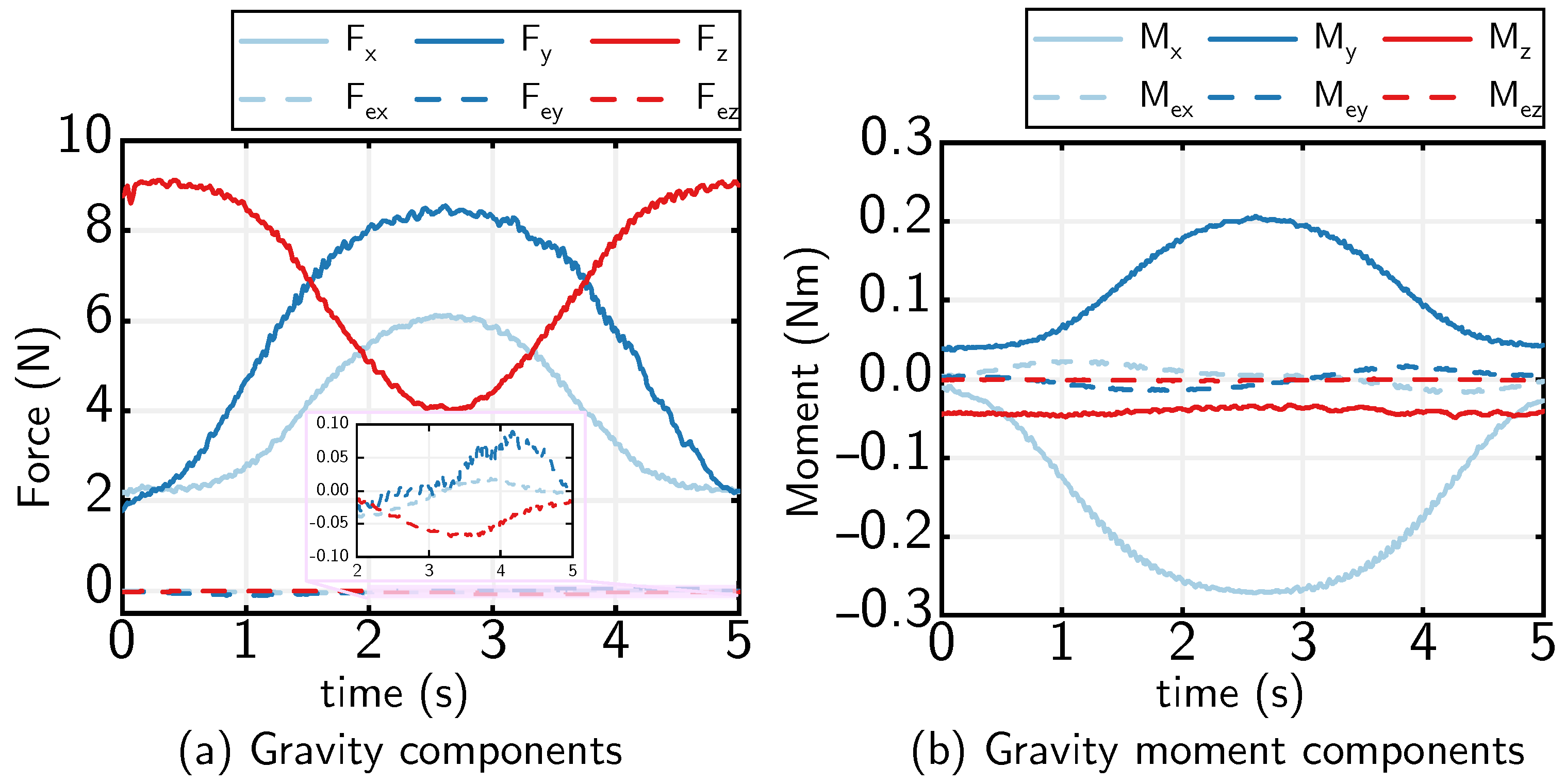
4. 6-Dof Force Sensor Gravity Compensation Strategy

The gravity of the grinding tool generates components of force and moment in the sensor coordinate system. The force and moment $F_m$ measured with the 6-Dof force sensor include: The grinding force $F_e$ between the grinding tool and the workpiece, the gravity of the grinding tool $F_G$, the inertial force $F_i$ generated by the grinding tool because of the movement (since the feed speed of the grinding tool changes very little, so that $F_i=0$), and the sensor zero drift $F_0$:

$${}^S{F}_m={}^S{F}_e+{}^S{F}_G+{}^S{F}_i+{}^S{F}_0$$

(35)

where the superscript ${}^S•$ indicates that the reference coordinate system of the force is in the sensor coordinate system $\left\{\mathrm{S}\right\}$.

Figure 7 shows the relationship between the world coordinate system $\left\{\mathrm{D}\right\}$, the robot base coordinate system $\left\{\mathrm{B}\right\}$, the end flange coordinate system $\left\{\mathrm{E}\right\}$, the force sensor coordinate system $\left\{\mathrm{S}\right\}$, and the grinding tool coordinate system $\left\{\mathrm{T}\right\}$. The barycenter of the grinding tool is represented as ${}^{S}o(x,y,z)$ in the $\left\{\mathrm{S}\right\}$ system. Using pins to maintain the parallel relationship between the axes of the $\left\{\mathrm{S}\right\}$ and $\left\{\mathrm{E}\right\}$ system, the homogeneous transformation matrix ${}_S^{B}T$ from $\left\{\mathrm{S}\right\}$ to $\left\{\mathrm{B}\right\}$ is:

$${}_S^{B}T=\left[\begin{array}{cc}{}_S^{B}R& {}_S^{B}P\\ 0& 1\end{array}\right]$$

(36)

where ${}_S^{B}R$ is the rotation matrix and ${}_S^{B}P$ is the vector of the sensor origin in the $\left\{\mathrm{S}\right\}$ system.

When there is no contact between the grinding tool and the workpiece, the sensor output signal is composed of the tool gravity and the sensor zero drift:

$$\left\{\begin{array}{c}{}^S{F}_{mx}={}^S{F}_{Gx}+F_{x0}\hfill \\ {}^S{F}_{my}={}^S{F}_{Gy}+F_{y0}\hfill \\ {}^S{F}_{mz}={}^S{F}_{Gz}+F_{z0}\hfill \\ {}^S{M}_{mx}={}^S{M}_{Gx}+M_{x0}\hfill \\ {}^S{M}_{my}={}^S{M}_{Gy}+M_{y0}\hfill \\ {}^S{M}_{mz}={}^S{M}_{Gz}+M_{z0}\hfill \end{array}\right.$$

(37)

where ${}^S{F}_{mx},{}^S{F}_{my},{}^S{F}_{mz},{}^S{M}_{mx},{}^S{M}_{my}$ and ${}^S{M}_{mz}$ are the force and moment signals of the 6-Dof force sensor, respectively.

Using the tool gravity and barycenter to obtain the torque that acts on the $\left\{\mathrm{S}\right\}$ system of the force sensor:

$$\left\{\begin{array}{c}{}^S{M}_{mx}={}^S{F}_{mz}y-{}^S{F}_{my}z+M_{x0}+F_{y0}z-F_{z0}y\hfill \\ {}^S{M}_{my}={}^S{F}_{mx}z-{}^S{F}_{mz}x+M_{y0}+F_{z0}x-F_{x0}z\hfill \\ {}^S{M}_{mz}={}^S{F}_{my}x-{}^S{F}_{mx}y+M_{z0}+F_{x0}y-F_{y0}x\hfill \end{array}\right.$$

(38)

Rewriting Equation (38) in matrix form:

$${}^S{M}_m={}^S{F}_m·A$$

(39)

where $A={\left[x,y,z,a_1,a_2,a_3\right]}^T,\left\{\begin{array}{c}{a}_1=M_{x0}+F_{y0}z-F_{z0}y\hfill \\ a_2=M_{y0}+F_{z0}x-F_{x0}z\hfill \\ a_3=M_{z0}+F_{x0}y-F_{y0}x\hfill \end{array}\right.$, ${}^S{F}_m=\left[\begin{array}{cccccc}0& {}^S{F}_{mz}& -{}^S{F}_{my}& 1& 0& 0\\ -{}^S{F}_{mz}& 0& {}^S{F}_{mx}& 0& 1& 0\\ {}^S{F}_{my}& -{}^S{F}_{mx}& 0& 0& 0& 1\end{array}\right]$

Selecting N different poses of the robot and using the least squares solution:

$$A={\left({}^{\mathrm{S}}{F}_m^{\mathrm{T}}·{}^{\mathrm{S}}{F}_m\right)}^{-1}·{}^{\mathrm{S}}{F}_m^{\mathrm{T}}·{}^{\mathrm{S}}{M}_m$$

(40)

The coordinate value $x,y,z$ of tool barycenter and constant $a_1,a_2,a_3$ in $\left\{\mathrm{S}\right\}$ system is obtained.

To obtain the component of the grinding tool in the $\left\{\mathrm{B}\right\}$ system, it is necessary to consider the relationship between the $\left\{\mathrm{B}\right\}$ system and the $\left\{\mathrm{D}\right\}$ system. When the $\left\{\mathrm{B}\right\}$ system rotates around the z axis of the $\left\{\mathrm{D}\right\}$ system, there is no effect on the force sensor output. Consider that the $\left\{\mathrm{B}\right\}$ system rotates around the x-axis and the y-axis of the $\left\{\mathrm{D}\right\}$ system. Then, the rotation matrix ${}_B^{D}R$ between the $\left\{\mathrm{B}\right\}$ system and the $\left\{\mathrm{D}\right\}$ system is:

$${}_B^{D}R=\left[\begin{array}{ccc}1& 0& 0\\ 0& cos{\theta }_1& -sin{\theta }_1\\ 0& sin{\theta }_1& cos{\theta }_1\end{array}\right]·\left[\begin{array}{ccc}cos{\theta }_2& 0& sin{\theta }_2\\ 0& 1& 0\\ -sin{\theta }_2& 0& cos{\theta }_2\end{array}\right]$$

(41)

where ${\theta }_1$ and ${\theta }_2$ are the angle around the x-axis and y-axis of the $\left\{\mathrm{D}\right\}$ system, respectively.

The component force of the grinding tool gravity G in the $\left\{\mathrm{S}\right\}$ system can be represented by the robot homogeneous transformation matrix:

$${}^{S}G=\left[\begin{array}{c}{}^S{F}_{Gx}\\ {}^S{F}_{Gy}\\ {}^S{F}_{Gz}\end{array}\right]={}_B^S{R}_D^B{R}^{D}G={}_B^{S}R\left[\begin{array}{c}Gcos{\theta }_{1}sin{\theta }_2\\ -Gsin{\theta }_1\\ -Gcos{\theta }_{1}cos{\theta }_2\end{array}\right]$$

(42)

Let $\left\{\begin{array}{c}{b}_x=Gcos{\theta }_{1}sin{\theta }_2\hfill \\ b_y=-Gsin{\theta }_1\hfill \\ b_z=-Gcos{\theta }_{1}cos{\theta }_2\hfill \end{array}\right.$.

According to Equation (37) and Equation (42):

$$\left[\begin{array}{c}{}^S{F}_{mx}\\ {}^S{F}_{my}\\ {}^S{F}_{mz}\end{array}\right]=\left[\begin{array}{c}{}^S{F}_{Gx}\\ {}^S{F}_{Gy}\\ {}^S{F}_{Gz}\end{array}\right]+\left[\begin{array}{c}{F}_{x0}\\ F_{y0}\\ F_{z0}\end{array}\right]={}_S^B{R}^T\left[\begin{array}{c}{b}_x\\ b_y\\ b_z\end{array}\right]+\left[\begin{array}{c}{F}_{x0}\\ F_{y0}\\ F_{z0}\end{array}\right]$$

(43)

Rewriting Equation (43) in matrix form:

$$\left[\begin{array}{c}{}^S{F}_{mx}\\ {}^S{F}_{my}\\ {}^S{F}_{mz}\end{array}\right]=\left[\begin{array}{c}{}_S^B{R}^T\mid I\hfill \end{array}\right]\left[\begin{array}{c}{b}_x\\ b_y\\ b_z\\ F_{x0}\\ F_{y0}\\ F_{z0}\end{array}\right]$$

(44)

Taking N different poses, we use Equation (44) to construct the equations and rewrite them as:

$${}^S{F}_m={}_S^B{R}_I·B$$

(45)

The least square solution of Equation (45) can be obtained as:

$$B={\left({}_S^B{R}_I^T{}_S^B{R}_I\right)}^{-1}·{}_S^B{R}_I^T·{}^S{F}_m$$

(46)

Then, the constant value of $b_x,b_y,b_z,F_{x0},F_{y0}$ and $F_{z0}$ is solved and, combined with Equation (39), the torque zero drift values ${}^S{M}_{mx0},{}^S{M}_{my0}$ and ${}^S{M}_{mz0}$ of the 6-Dof force sensor can be obtained.

The gravity of the grinding tool is as follows: $G=\sqrt{b_x^2+b_y^2+b_z^2}$.

The angle value between the $\left\{\mathrm{B}\right\}$ system and the $\left\{\mathrm{D}\right\}$ system is as follows: ${\theta }_1=arcsin\left(-\frac{b_y}{g}\right)$, ${\theta }_2=arcsin\left(-\frac{b_x}{b_z}\right)$.

The identification results in

Table 1. The result of end effector gravity identification.

Gravity (N)	x (m)	y (m)	z (m)	${\mathit{\theta }}_1$ (${}^{\circ }$)	${\mathit{\theta }}_2$ (${}^{\circ }$)
8.956	−0.0020	−0.0053	0.0455	0.8052	1.8096

and

Table 2. The result of sensor zero drift identification.

Zero Drift	${\mathit{F}}_{\mathit{x}0}$ (N)	${\mathit{F}}_{\mathit{y}0}$ (N)	${\mathit{F}}_{\mathit{z}0}$ (N)	${\mathit{M}}_{\mathit{x}0}$ (Nm)	${\mathit{M}}_{\mathit{y}0}$ (Nm)	${\mathit{M}}_{\mathit{z}0}$ (Nm)
Value	0.6382	−0. 4779	0.5209	0.0295	0.0134	−0.0379

were obtained by selecting 10 groups of poses. The true gravity of the grinding tool is 8.542 N, which is only 0.414 N different from the identification result. We selected a trajectory and performed real-time gravity compensation. Figure 8 shows the compensation results; the maximum disturbance after compensation is less than 0.1 N and 0.03 N·m, which verifies the accuracy and effect of gravity compensation.

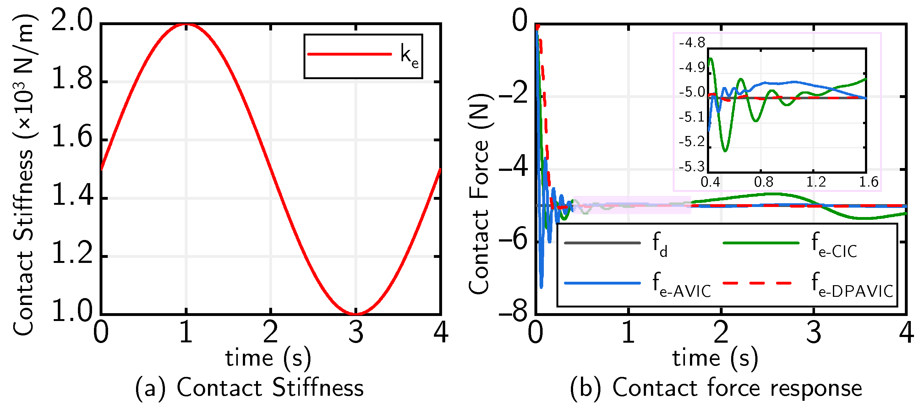
5. Controller Simulation Verification

Constant impedance control (CIC), adaptive variable impedance control (AVIC), and DPAVIC algorithms were used to verify the superiority and feasibility of the methods. The simulation system was established in MATLAB R2022b/Simulink, and the robot toolbox was used to establish the dynamics model of Franka Emika Panda.

Table 3. Simulation parameters.

Parameters	Value
$m\left(\mathrm{kg}\right)$	1.0
$b(\mathrm{N}/(\mathrm{m}/\mathrm{s}\left)\right)$	50
$k(\mathrm{N}/\mathrm{m})$	0
$k_e(\mathrm{N}/\mathrm{m})$	2000
$t_s\left(\mathrm{ms}\right)$	1

shows the simulation parameters.

The force control simulation was performed on the curved surface shown in Figure 9a. In the force controller, $k_p=0.6, k_d=0.4, k_i=0.01, \sigma =0.01, r=500, h=0.01$, and the desired force is $f_d=-5$ N. As can be seen in Figure 9b, the force tracking errors of CIC and AVIC both exceed the range of ±0.2 N. DPAVIC shows superior performance in the force tracking effect, and the force tracking error is within the range of ±0.2 N. Because the force overshoot is suppressed by NTD and PD in force tracking controllers, the overshoot of force is reduced from 52.34% to 8.3% compared with that in CIC. The force control effect is also simulated when the workpiece stiffness due to disturbance, as shown in Figure 10a, and it can be found from Figure 10b that both CIC and AVIC have large force fluctuations, while the force error of the method proposed in this paper is stable within the range of ±0.2 N. Therefore, the DPAVIC method can effectively compensate for the force tracking errors caused by position and stiffness disturbance.

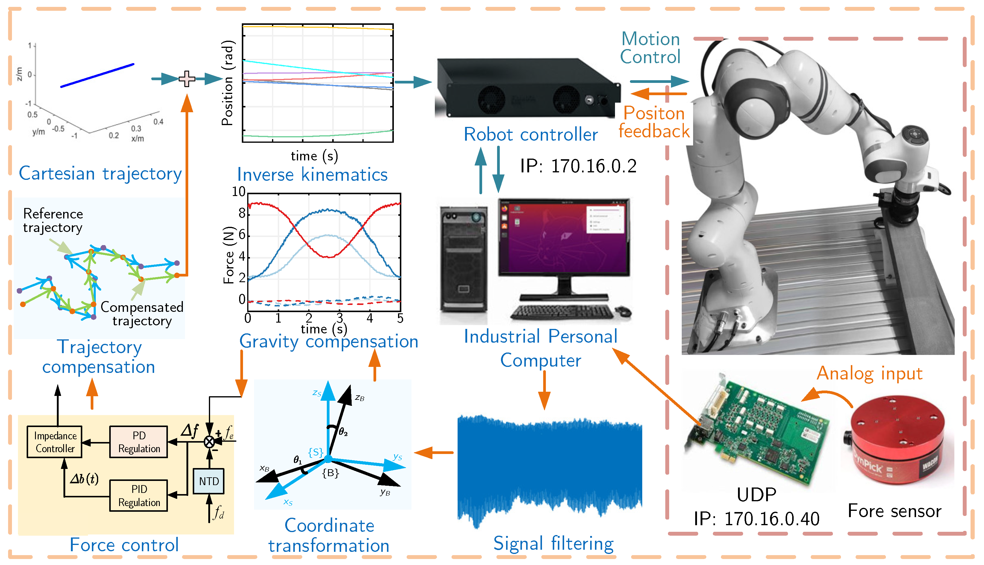
6. Experimental Study

To verify the performance of the proposed control strategy, a robot force control platform is established, as shown in Figure 11. Programming is performed in a MATLAB/Simulink environment using Simulink S-function block. The robot control frequency is 1KHz. The HKTECH NET6043-S analog IO module is connected to the robot controller through cables, the grinding force is read through the Simulink UDP module of the Industrial Personal Computer, and the grinding force signal is fed back to the robot control algorithm. Multiple groups of force control experiments are carried out on a flat surface, slope surface, and large curvature surface, respectively, as shown in Figure 12. Finally, the grinding experiment is carried out on a thin-wall aluminum alloy 7050-T6 workpiece. The results of CIC, AVIC, and DPAVIC on the end force tracking are discussed.

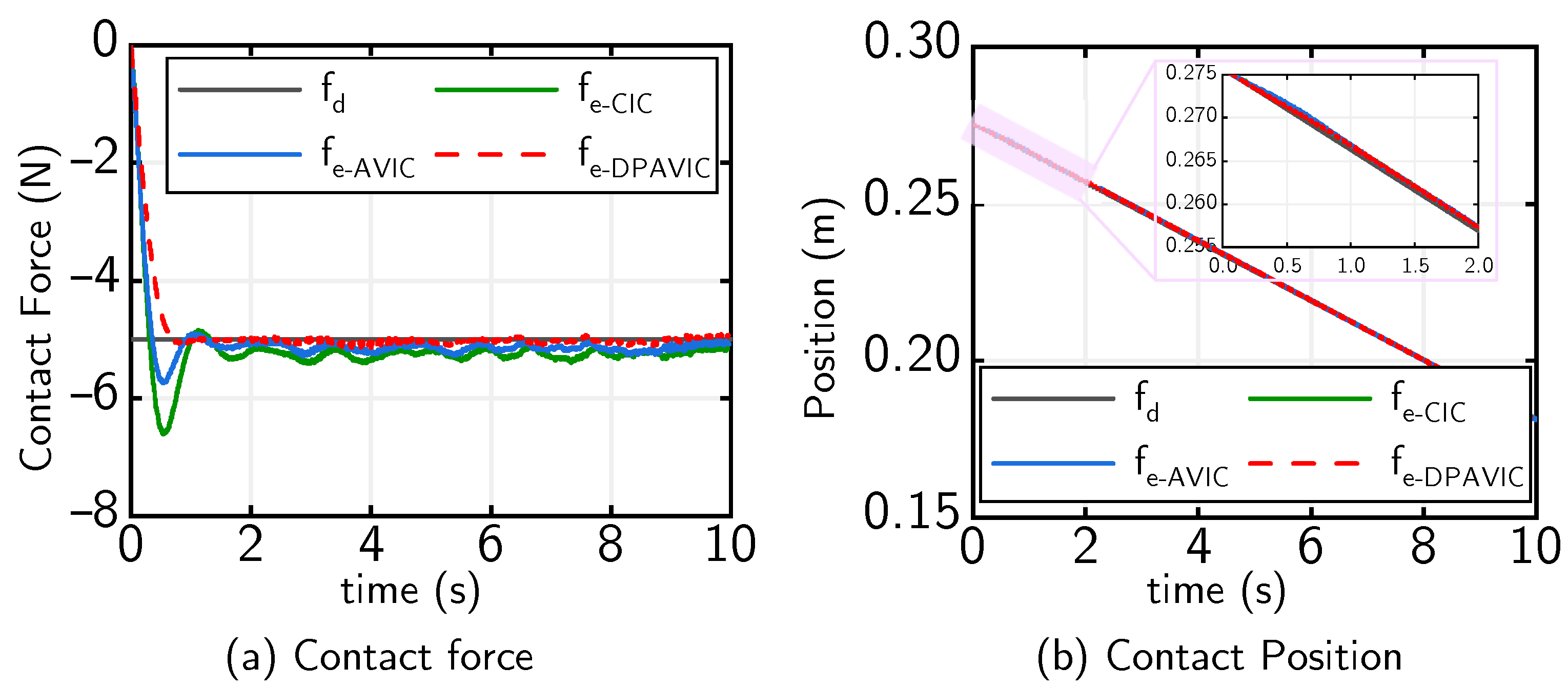
6.1. Flat Surface Constant Force Control

The force control experiment was carried out on a flat surface, as shown in Figure 12a. The end of the robot moved 0.3 m in the x direction, and the force control direction was in the z direction of the end effector. The desired force was set as $f_d=-5$ N, and the running time was 10 s. The control parameters of CIC, AVIC, and DPAVIC were set as follows:

CIC: $m=1,b=10,k=0$.

AVIC: $m=1,b=8,k=0,\sigma =0.003$.

DPAVIC: $m=1,b=5,k=0,\sigma =0.003,k_p=0.4,k_d=0.1,k_i=0.001,r=100$, $h=0.01$.

Figure 13 shows the robot end contact force control and end compensation displacement. It can be found that when CIC and AVIC are adopted, the overshoot of the system is large, 34.31% and 13.54% respectively, the force control error is 0.409 N and 0.25 N, and the adjustment time is long. When the DPAVIC force control strategy is adopted, the overshoot is 1.35% and the force control error is within ±0.2 N.

6.2. Slope Surface Constant Force Control

The end contact force was controlled on the slope surface shown in Figure 12b. The desired force was set as $f_d=-5$ N and the running time was 10 s. The control parameters of the CIC, AVIC, and DPAVIC methods were set as follows:

CIC: $m=1,b=8,k=0$.

AVIC: $m=1,b=5,k=0,\sigma =0.003$.

DPAVIC: $m=1,b=5,k=0,\sigma =0.005,k_p=0.4,k_d=0.05,k_i=0.001,r=100$, $h=0.01$.

Figure 14 shows the control response curves of the end compensation displacement and the end contact force. It can be found that when CIC and AVIC are used, the overshoot of the system is 29.46% and 12.45%, respectively, and the force control error is 0.331 N and 0.247 N. When the DPAVIC force control strategy is adopted, the overshoot is less than 1.02%, and the error is within ±0.2 N.

6.3. Large Curvature Surface Constant Force Control

To ensure the force control effectiveness of the force control algorithm for curved surface parts, the force control platform shown in Figure 12c was adopted. The desired contact force was set as $f_d=-5$ N and the running time was 10 s. The control parameters of the CIC, AVIC, and DPAVIC methods were set as:

CIC: $m=1,b=8,k=0$.

AVIC: $m=1,b=8,k=0,\sigma =0.003$.

DPAVIC: $m=1,b=5,k=0,\sigma =0.01,k_p=0.2,k_d=0.05,k_i=0.001,r=100,$ $h=0.01$.

Figure 15 shows the response curves of the end compensation displacement and the contact force. It can be found that when CIC and AVIC are adopted, the overshoot of the system is large, 10.26% and 7.25%, respectively, and the force control error is 0.336 N and 0.252 N. However, the overshoot and force error of DPAVIC are 1.51%, within ±0.2 N, respectively. Although the system response is slow with the DPAVIC method, the adjustment time is shorter.

6.4. Constant Force Grinding Experiment

According to the geometric model of the workpiece surface, the Cartesian space trajectory is planned, the specific grinding pose of the robot end effector is deduced via interpolation with the given feed speed, and the grinding trajectory of the joint space is obtained online with the inverse differential kinematics of the robot. According to the on-site machining requirements, the surface quality of the workpiece should be below Ra 0.3 $\mathsf{\mu }$m, the reference grinding force is 5 N, and the force fluctuation is ±0.2 N.

Table 4. Grinding process parameters.

Feed Rate (mm/s)	Grinding Tool Diameter (mm)	Sandpaper (grit)	Grinding Tool Speed (rpm)	(${\mathit{F}}_{\mathit{d}}$) (N)
15	50	100	3000	−5

shows the grinding process parameters. The CIC, AVIC, and DPAVIC control parameters are set to the same as the flate force control parameters.

As can be seen from Figure 16, the force error in the CIC force tracking control method is far more than ±0.2 N, and the force control result of AVIC is slightly better than that of CIC, while the error of the DPAVIC method stays within ±0.2 N. This proves the ability of the method to improve the precision of force control.

Figure 17 shows the robot grinding process and the surface quality of the workpiece after grinding. To verify the effectiveness of the proposed method for improving machining quality, a JiTai TR200S roughometer was used to measure the surface roughness of the workpiece, a Dino-Lite microscope was used to photograph the grinding surface morphology, and a Mitotoyo Roughness Meter SJ-210 was used to measure surface waviness. As shown in Figure 17b, 10 points on the workpiece surface are selected and the average of three measurements is taken.

Figure 18 shows the measured roughness of the workpiece. Compared with the CIC method, the average surface quality of the workpiece is improved from Ra 0.5 $\mathsf{\mu }$m to Ra 0.218 $\mathsf{\mu }$m. Figure 19 shows the influence of the three force control methods on the workpiece surface waviness. Figure 19a shows that when using the CIC method, the workpiece surface waviness fluctuates with the grinding force oscillation. Figure 19b shows a slight reduction in waviness with AVIC compared with the CIC method. Figure 19c shows the ability of the DPAVIC method to reduce the workpiece surface waviness, which has the lowest waviness compared with the other two methods. Therefore, the proposed method has the ability to suppress the external disturbance and reduce the force tracking error and fluctuation.

7. Conclusions

Force control is an important problem in robot contact operation. In order to achieve high efficiency and high-quality robot grinding, a position-based dual PID adaptive variable impedance control method is proposed, PD is used to compensate for the force error, and PID is used to update the impedance parameters to compensate for the environmental disturbance. An overshoot suppression strategy using a nonlinear tracking differentiator is presented to smooth the desired force and reduce the contact force overshoot. The disturbance term of the end force signal is identified using the least square method, and the effect of gravity compensation is verified to reduce the influence of noise on the force control accuracy. The stability, convergence, and effectiveness of the force control algorithm are verified via theoretical analysis, simulations, and experiments. By comparing the results of CIC, AVIC, and DPAVIC with the robot end force control accuracy, the DPAVIC method can be maintained within ±0.2 N, and it has high anti-interference ability. The surface roughness of the thin-walled workpiece can be improved to Ra 0.218 $\mathsf{\mu }$m.

In future work, we will consider how to use force sensors to intelligently sense changes in workpiece surface curvature without geometric models and achieve compliant grinding of the workpiece.

References

1. Zhu, D.; Feng, X.; Xu, X.; Yang, Z.; Li, W.; Yan, S.; Ding, H. Robotic grinding of complex components: A step towards efficient and intelligent machining–challenges, solutions, and applications. Robot. Comput.-Integr. Manuf. 2020, 65, 101908. [Google Scholar] [CrossRef]
2. Zhu, W.L.; Beaucamp, A. Compliant grinding and polishing: A review. Int. J. Mach. Tools Manuf. 2020, 158, 103634. [Google Scholar] [CrossRef]
3. Ma, K.; Yang, G. Kinematic design of a 3-DOF force-controlled end-effector module. In Proceedings of the 2016 IEEE 11th Conference on Industrial Electronics and Applications (ICIEA), Hefei, China, 5–7 June 2016; pp. 1084–1089. [Google Scholar]
4. Mu, Y.; Wang, Z.; Zou, L.; Wang, W.; Lv, C.; Wang, A. A novel regional force control strategy based on seven-axis linkage grinding system to improve blade machining accuracy. J. Manuf. Process. 2023, 97, 235–247. [Google Scholar] [CrossRef]
5. Solanes, J.E.; Gracia, L.; Muñoz-Benavent, P.; Valls Miro, J.; Perez-Vidal, C.; Tornero, J. Robust hybrid position-force control for robotic surface polishing. J. Manuf. Sci. Eng.-Trans. ASME 2019, 141, 011013. [Google Scholar] [CrossRef]
6. Mohammad, A.E.K.; Hong, J.; Wang, D. Design of a force-controlled end-effector with low-inertia effect for robotic polishing using macro-mini robot approach. Robot. Comput.-Integr. Manuf. 2018, 49, 54–65. [Google Scholar] [CrossRef]
7. Gracia, L.; Solanes, J.E.; Munoz-Benavent, P.; Miro, J.V.; Perez-Vidal, C.; Tornero, J. Adaptive sliding mode control for robotic surface treatment using force feedback. Mechatronics 2018, 52, 102–118. [Google Scholar] [CrossRef]
8. Zhang, H.; Li, L.; Zhao, J.; Zhao, J. The hybrid force/position anti-disturbance control strategy for robot abrasive belt grinding of aviation blade base on fuzzy PID control. Int. J. Adv. Manuf. Technol. 2021, 114, 3645–3656. [Google Scholar] [CrossRef]
9. Kakinuma, Y.; Ogawa, S.; Koto, K. Robot polishing control with an active end effector based on macro-micro mechanism and the extended Preston’s law. CIRP Ann.-Manuf. Technol. 2022, 71, 341–344. [Google Scholar] [CrossRef]
10. Chang, G.; Pan, R.; Xie, Y.; Yang, J.; Yang, Y.; Li, J. Research on constant force polishing method of curved mold based on position adaptive impedance control. Int. J. Adv. Manuf. Technol. 2022, 122, 697–709. [Google Scholar] [CrossRef]
11. Rosales, A.; Heikkilä, T. Analysis and Design of Direct Force Control for Robots in Contact with Uneven Surfaces. Appl. Sci. 2023, 13, 7233. [Google Scholar] [CrossRef]
12. Zhou, H.; Ma, S.; Wang, G.; Deng, Y.; Liu, Z. A hybrid control strategy for grinding and polishing robot based on adaptive impedance control. Adv. Mech. Eng. 2021, 13, 16878140211004034. [Google Scholar] [CrossRef]
13. Xu, X.; Chen, W.; Zhu, D.; Yan, S.; Ding, H. Hybrid active/passive force control strategy for grinding marks suppression and profile accuracy enhancement in robotic belt grinding of turbine blade. Robot. Comput.-Integr. Manuf. 2021, 67, 102047. [Google Scholar] [CrossRef]
14. Su, X.; Xie, Y.; Sun, L.; Jiang, B. Constant Force Control of Centrifugal Pump Housing Robot Grinding Based on Pneumatic Servo System. Appl. Sci. 2022, 12, 9708. [Google Scholar] [CrossRef]
15. Ke, X.; Yu, Y.; Li, K.; Wang, T.; Zhong, B.; Wang, Z.; Kong, L.; Guo, J.; Huang, L.; Idir, M.; et al. Review on robot-assisted polishing: Status and future trends. Robot. Comput.-Integr. Manuf. 2023, 80, 102482. [Google Scholar] [CrossRef]
16. Al-Shuka, H.F.; Leonhardt, S.; Zhu, W.H.; Song, R.; Ding, C.; Li, Y. Active impedance control of bioinspired motion robotic manipulators: An overview. Appl. Bionics Biomech. 2018, 2018, 8203054. [Google Scholar] [CrossRef] [PubMed]
17. Fan, C.; Hong, G.S.; Zhao, J.; Zhang, L.; Zhao, J.; Sun, L. The integral sliding mode control of a pneumatic force servo for the polishing process. Precis. Eng.-J. Int. Soc. Precis. Eng. Nanotechnol. 2019, 55, 154–170. [Google Scholar] [CrossRef]
18. Ma, Z.; Poo, A.N.; Ang, M.H., Jr.; Hong, G.S.; See, H.H. Design and control of an end-effector for industrial finishing applications. Robot. Comput.-Integr. Manuf. 2018, 53, 240–253. [Google Scholar] [CrossRef]
19. Li, J.; Guan, Y.S.; Chen, H.W.; Wang, B.; Zhang, T.; Liu, X.N.; Hong, J.; Wang, D.W.; Zhang, H. A high-bandwidth end-effector with active force control for robotic polishing. IEEE Access 2020, 8, 169122–169135. [Google Scholar] [CrossRef]
20. Dai, J.; Chen, C.Y.; Zhu, R.; Yang, G.; Wang, C.; Bai, S. Suppress vibration on robotic polishing with impedance matching. Actuators 2021, 10, 59. [Google Scholar] [CrossRef]
21. Nguyen, V.L.; Kuo, C.H.; Lin, P.T. Compliance error compensation of a robot end-effector with joint stiffness uncertainties for milling: An analytical model. Mech. Mach. Theory 2022, 170, 104717. [Google Scholar] [CrossRef]
22. Yang, G.; Zhu, R.; Fang, Z.; Chen, C.Y.; Zhang, C. Kinematic design of a 2R1T robotic end-effector with flexure joints. IEEE Access. 2020, 8, 57204–57213. [Google Scholar] [CrossRef]
23. Jin, M.; Ji, S.; Pan, Y.; Ao, H.; Han, S. Effect of downward depth and inflation pressure on contact force of gasbag polishing. Precis. Eng.-J. Int. Soc. Precis. Eng. Nanotechnol. 2017, 47, 81–89. [Google Scholar] [CrossRef]
24. Chen, Y.; Zhao, J.; Jin, Y. An improved rational Bezier model for pneumatic constant force control device of robotic polishing with hysteretic nonlinearity. Int. J. Adv. Manuf. Technol. 2022, 123, 665–674. [Google Scholar] [CrossRef]
25. Pei, G.; Yu, M.; Xu, Y.; Ma, C.; Lai, H.; Chen, F.; Lin, H. An improved PID controller for the compliant constant-force actuator based on BP neural network and smith predictor. Appl. Sci. 2021, 11, 2685. [Google Scholar] [CrossRef]
26. Chen, H.; Yang, J.; Ding, H. Robotic compliant grinding of curved parts based on a designed active force-controlled end-effector with optimized series elastic component. Robot. Comput.-Integr. Manuf. 2024, 86, 102646. [Google Scholar] [CrossRef]
27. Chen, P.; Zhao, H.; Yan, X.; Ding, H. Force control polishing device based on fuzzy adaptive impedance control. In Proceedings of the Intelligent Robotics and Applications: 12th International Conference, ICIRA 2019, Shenyang, China, 8–11 August 2019; Proceedings, Part IV 12. Springer: Berlin/Heidelberg, Germany, 2019; pp. 181–194. [Google Scholar]
28. Wei, Y.; Xu, Q. Design of a new passive end-effector based on constant-force mechanism for robotic polishing. Robot. Comput.-Integr. Manuf. 2022, 74, 102278. [Google Scholar] [CrossRef]
29. Chen, F.; Zhao, H.; Li, D.; Chen, L.; Tan, C.; Ding, H. Contact force control and vibration suppression in robotic polishing with a smart end effector. Robot. Comput.-Integr. Manuf. 2019, 57, 391–403. [Google Scholar] [CrossRef]
30. Wang, Q.; Wang, W.; Ding, X.; Yun, C. A force control joint for robot–environment contact application. J. Mech. Robot. 2019, 11, 034502. [Google Scholar] [CrossRef]
31. Chen, C.Y.; Dai, J.; Yang, G.; Wang, C.; Li, Y.; Chen, L. Sensor-based force decouple controller design of macro–mini manipulator. Robot. Comput.-Integr. Manuf. 2023, 79, 102415. [Google Scholar] [CrossRef]
32. Xie, F.; Chong, Z.; Liu, X.J.; Zhao, H.; Wang, J. Precise and smooth contact force control for a hybrid mobile robot used in polishing. Robot. Comput.-Integr. Manuf. 2023, 83, 102573. [Google Scholar] [CrossRef]
33. Hogan, N. Impedance control: An approach to manipulation. In Proceedings of the 1984 American Control Conference, San Diego, CA, USA, 6–8 June 1984; pp. 304–313. [Google Scholar]
34. Gu, L.; Huang, Q. Adaptive Impedance Control for Force Tracking in Manipulators Based on Fractional-Order PID. Appl. Sci. 2023, 13, 10267. [Google Scholar] [CrossRef]
35. Kawamura, S. Hybrid position/force control of robot manipulators based on learning method. In Proceedings of the 2nd International Conference on Advanced Robotics ICAR 85, Tokyo, Japan, 9–10 September 1985. [Google Scholar]
36. Gan, Y.; Duan, J.; Chen, M.; Dai, X. Multi-robot trajectory planning and position/force coordination control in complex welding tasks. Appl. Sci. 2019, 9, 924. [Google Scholar] [CrossRef]
37. Li, L.; Wang, Z.; Zhu, G.; Zhao, J. Position-based force tracking adaptive impedance control strategy for robot grinding complex surfaces system. J. Field Robot. 2023, 40, 1097–1114. [Google Scholar] [CrossRef]
38. Seraji, H.; Colbaugh, R. Force tracking in impedance control. Int. J. Robot. Res. 1997, 16, 97–117. [Google Scholar] [CrossRef]
39. Bilal, M.; Akram, M.N.; Rizwan, M. Adaptive Variable Impedance Control for Multi-axis Force Tracking in Uncertain Environment Stiffness with Redundancy Exploitation. Control Eng. Appl. Inform. 2022, 24, 35–45. [Google Scholar]
40. Jia, H.; Lu, X.; Cai, D.; Xiang, Y.; Chen, J.; Bao, C. Predictive Modeling and Analysis of Material Removal Characteristics for Robotic Belt Grinding of Complex Blade. Appl. Sci. 2023, 13, 4248. [Google Scholar] [CrossRef]
41. Kronander, K.; Billard, A. Stability considerations for variable impedance control. IEEE Trans. Robot. 2016, 32, 1298–1305. [Google Scholar] [CrossRef]
42. Cao, H.; Chen, X.; He, Y.; Zhao, X. Dynamic adaptive hybrid impedance control for dynamic contact force tracking in uncertain environments. IEEE Access. 2019, 7, 83162–83174. [Google Scholar] [CrossRef]
43. Wang, G.; Deng, Y.; Zhou, H.; Yue, X. PD-adaptive variable impedance constant force control of macro-mini robot for compliant grinding and polishing. Int. J. Adv. Manuf. Technol. 2023, 124, 2149–2170. [Google Scholar] [CrossRef]
44. Wahballa, H.; Duan, J.; Dai, Z. Constant force tracking using online stiffness and reverse damping force of variable impedance controller for robotic polishing. Int. J. Adv. Manuf. Technol. 2022, 121, 5855–5872. [Google Scholar] [CrossRef]
45. Wang, Q.; Wang, W.; Zheng, L.; Yun, C. Force control-based vibration suppression in robotic grinding of large thin-wall shells. Robot. Comput.-Integr. Manuf. 2021, 67, 102031. [Google Scholar] [CrossRef]
46. Lee, C.H.; Wang, W.C. Robust adaptive position and force controller design of robot manipulator using fuzzy neural networks. Nonlinear Dyn. 2016, 85, 343–354. [Google Scholar] [CrossRef]
47. Irawan, A.; Nonami, K. Optimal impedance control based on body inertia for a hydraulically driven hexapod robot walking on uneven and extremely soft terrain. J. Field Robot. 2011, 28, 690–713. [Google Scholar] [CrossRef]
48. Ranko, Z.; Angel, V.F.; Pedro, G.G.; Angel, L.G. An architecture for robot force and impact control. In Proceedings of the 2006 IEEE Conference on Robotics, Automation and Mechatronics, Bangkok, Thailand, 7–9 June 2006; pp. 1–6. [Google Scholar]
49. Roveda, L.; Pedrocchi, N.; Vicentini, F.; Tosatti, L.M. An interaction controller formulation to systematically avoid force overshoots through impedance shaping method with compliant robot base. Mechatronics 2016, 39, 42–53. [Google Scholar] [CrossRef]
50. Duan, J.; Gan, Y.; Chen, M.; Dai, X. Adaptive variable impedance control for dynamic contact force tracking in uncertain environment. Robot. Auton. Syst. 2018, 102, 54–65. [Google Scholar] [CrossRef]
Figure 1. Robot grinding force control system.
Applsci 13 11635 g001
Figure 2. Contact behavior between robot and external environment. (a) No contact. (b) Critical point of contact. (c) The contact state. (d) The contact force during the contact process.
Applsci 13 11635 g002
Figure 3. Robot end-contact-force transition state control.
Applsci 13 11635 g003
Figure 4. Simulation and experimental results of robot end contact state transition.
Applsci 13 11635 g004
Figure 5. The state of contact between the workpiece and the end effector.
Applsci 13 11635 g005
Figure 6. Dual PID adaptive variable impedance control.
Applsci 13 11635 g006
Figure 7. Gravity compensation modeling.
Applsci 13 11635 g007
Figure 8. Comparison of sensor signals before ( F , M ) and after ( F e , M e ) compensation.
Applsci 13 11635 g008
Figure 9. Force tracking results of curved surface.
Applsci 13 11635 g009
Figure 10. Force tracking results with the stiffness disturbance.
Applsci 13 11635 g010
Figure 11. Experimental setup for robot grinding force control.
Applsci 13 11635 g011
Figure 12. Force control platform.
Applsci 13 11635 g012
Figure 13. Force control results of flat surface.
Applsci 13 11635 g013
Figure 14. Force control results of slope surface.
Applsci 13 11635 g014
Figure 15. Force control results of large curvature surface.
Applsci 13 11635 g015
Figure 16. Contact force signal during grinding.
Applsci 13 11635 g016
Figure 17. Workpiece grinding quality.
Applsci 13 11635 g017
Figure 18. Workpiece surface roughness.
Applsci 13 11635 g018
Figure 19. Workpiece surface waviness. (a) Effect of CIC on workpiece surface waviness. (b) Effect of AVIC on workpiece surface waviness. (c) Effect of DPAVIC on workpiece surface waviness.
Applsci 13 11635 g019