Carbon Dioxide Fluxes and Influencing Factors in the Momoge Salt Marsh Ecosystem, Jilin Province, China

Abstract

This study observed the characteristics and influencing factors of the carbon fluxes of the Momoge salt marsh ecosystem over four years, which behaves as a CO₂ sink. The daily, seasonal, and interannual variations in CO₂ fluxes in the Momoge salt marshes were observed using the eddy covariance method and were compared with various environmental factors. An overall daily “U”-shaped distribution was observed, with uptake during the day (negative values) and release at night (positive values). Annually, the carbon fluxes in the study area roughly exhibited a “V” shape. The carbon fluxes during the non-growing season predominantly showed positive values, indicating the release of CO₂ into the atmosphere. Photosynthetically active radiation was the primary influencing factor affecting the hourly and daytime variations in net ecosystem exchange (NEE) during the growing season, while temperature was the main factor influencing nighttime NEE dynamics. The air temperature, soil temperature, photosynthetically active radiation, precipitation, and water level all had significant impacts on the daily net CO₂ exchange. At the monthly scale, larger values of soil temperature, air temperature, photosynthetically active radiation, and aboveground biomass corresponded to a stronger carbon absorption capacity of the ecosystem. Overall, temperature remains the primary factor for carbon fluxes in the Momoge wetlands.

1. Introduction

Quantitative research on the balance of global greenhouse gases and their control mechanisms has become a focus among global environmental science research programs. Notable programs that are dedicated to addressing this issue include the International Geosphere-Biosphere Program, the World Climate Research Program, the International Human Dimensions Program on Global Environmental Change, and Global Change and Terrestrial Ecosystems. Wetland ecosystems play a crucial role in the global carbon cycle. Among the five major terrestrial ecosystems closely linked to the global carbon cycle—forests, grasslands, croplands, wetlands, and inland waters—wetlands constitute the largest component of the carbon reservoir of the terrestrial biosphere [1]. Consequently, they play a vital role in the global carbon cycle [2,3]. The total global area of wetlands is approximately 5.7 × 10⁶ km². This accounts for approximately 6% of the Earth’s land area, which is significantly lower than the area covered by forests; however, due to their high productivity and redox potential, wetlands have become crucial sites for biogeochemical processes in the biosphere [4]. Owing to prolonged or intermittent waterlogging, the anaerobic conditions in wetlands inhibit the decomposition of detritus, leading to the accumulation of organic matter in the soil. As a result, wetlands are carbon sinks that mitigate the rise in atmospheric CO₂ concentrations. According to estimates by the Intergovernmental Panel on Climate Change, global terrestrial ecosystems store approximately 2.48 × 10⁶ TgC (1 Tg = 1 × 10¹² g), of which peatlands store around 0.5 × 10⁶ TgC. Peatlands alone store twice the carbon content of all forests combined, constituting 20% of the total carbon stock in global terrestrial ecosystems [5]. This indicates that wetland ecosystems have significant potential to mitigate global warming. Although they have substantial soil carbon reservoirs, they are also significant sources of methane emissions, accounting for more than 20% of the global annual methane emissions each year [6]. In the context of global warming, as soil moisture decreases and soil oxidation capacity intensifies, the anaerobic conditions in wetlands are mitigated. This leads to a significant acceleration of the decomposition rates of detritus and peat, resulting in an increase in CO₂ emissions, which can create a positive feedback mechanism that exacerbates global warming [7].

Reeds are widely distributed in various types of salt marshes because of their adaptability and high reproductive capacity. They are extensively cultivated in various countries because of their significant economic and ecological value. Numerous studies [8,9,10,11] indicate that peatlands and reed wetlands serve as crucial carbon sinks. However, the carbon sink function of wetlands is influenced by various factors, including hydrology, temperature, and atmospheric CO₂ concentrations as well as nutrients like nitrogen (N) and phosphorus (P). Hence, studying variations in carbon fluxes in reed wetlands is important for understanding the sources and sinks of greenhouse gases.

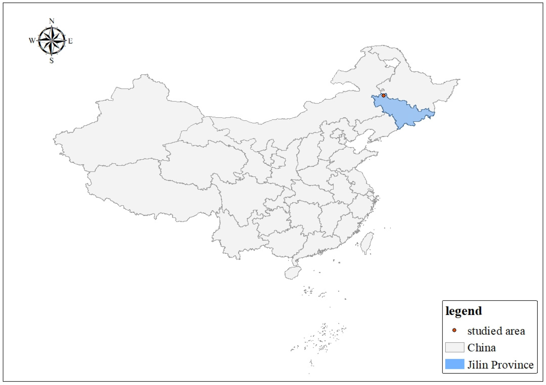
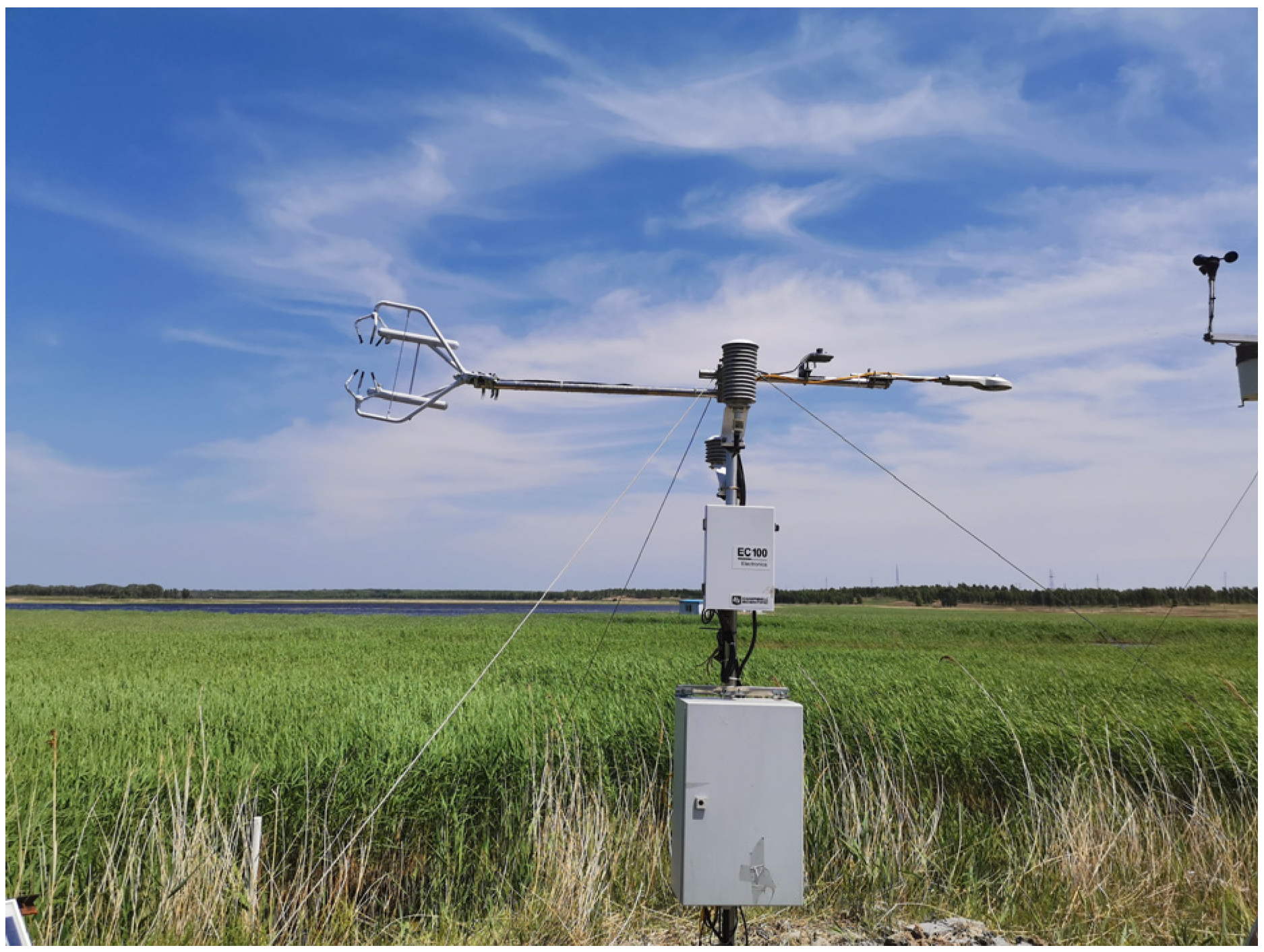
The Momoge salt marshes are located in Jilin Province, China, and are characterized by arid and semi-arid lands with fragile ecosystems. Natural hydrological changes and human disturbances contribute to significant spatiotemporal variability in greenhouse gas emissions. Reed marshes, as one of the widely distributed wetland types in the region, play a crucial role in wetland carbon balances. Currently, due to the limited direct observations of CO₂ exchange between reed marshes and the atmosphere, quantitatively analyzing the correlations between CO₂ fluxes and environmental factors remains difficult. This limits our understanding of various physical and chemical processes that influence carbon accumulation and cycling in reed marshes. Advancements in eddy covariance technology have made accurate measurements of carbon exchange in wetland ecosystems possible. This study is based on four years of data from eddy correlation flux towers and automated meteorological stations within the study area. By investigating the CO₂ fluxes in the Momoge salt marsh ecosystem, this study analyzes the daily, seasonal, and interannual variation in the net ecosystem exchange (NEE). Additionally, by exploring the correlations between net CO₂ exchanges and major environmental factors at both daily and monthly scales, the results provide new insights into the local climate characteristics and land–atmosphere interactions in the Momoge wetlands. These findings can provide localized and accurate data for climate change modeling, global ecosystem modeling, and developing strategies for reducing greenhouse gas emissions.

2. Materials and Methods

2.1. Overview of the Study Area

The study area is on Juzhi Island within the Momoge National Nature Reserve. It is situated in the southeastern part of Zhenlai County, Baicheng City, in the western Songnen Plain of Jilin Province (Figure 1). This area represents a typical wetland-type protected area and is the largest wetland conservation area in Jilin Province. It serves as a significant stopover site for waterbirds in the northern part of China’s eastern migratory route. The Momoge wetlands have a temperate continental monsoon climate. The average annual temperature in the area is 4.2 °C, with an average annual precipitation of 391.8 mm. The predominant soil types are marsh soil, meadow soil, black soil (chernozem), and alluvial soil. The region boasts abundant water resources, primarily sourced from the Nen River system. The intricate network of ponds, marshes, and lakes within the basin formed due to the confluence of the Tao’er River and the Nen River. In this study, we selected widely distributed reed marshes to conduct long-term carbon flux monitoring.

2.2. Flux Observations

An open-path eddy covariance system was installed in November 2014 in the Momoge wetlands. It was placed at a height of 2 m above the top of the vegetation. The vegetation within 1000 m around the instrument was dominated by reeds, with a sporadic distribution of balsam (Figure 2). The open-path eddy covariance system mainly consisted of an open-path infrared CO₂/H₂O analyzer (EC150), a three-dimensional ultrasonic anemometer (CS150, Campbell Scientific, Logan, UT, USA), and a data collector (CR3000, Campbell Scientific, USA). The infrared CO₂/H₂O analyzer and the three-dimensional ultrasonic anemometer were mounted on a long arm measuring about 1 m. They were fixed to the monitoring tower and oriented towards the direction of the prevailing winds throughout the year in order to reduce the effect of disturbances formed by the air at the tower on the instruments. The data collector collected 10 Hz raw data in real time, calculated the flux and other covariance data online using the EasyFlux-DL software, and recorded and stored the data on a PC card. As the sensor malfunctioned and was returned to the factory for repair in 2018, the range of data selected for this study included January 2015 to December 2017 and the full year of 2021.

2.3. Micrometeorological Observations

At the same time as the flux system installation, an automatic meteorological observation system (HOBO, Lakeville, MN, USA) was installed, which continuously and automatically monitored and stored ten parameters, namely, the local air temperature, relative humidity, wind speed, wind direction, soil temperature, soil moisture, total radiation, photosynthetically active radiation, barometric pressure, and rainfall. This facilitated the study of changes in the meteorological environment and their impacts on the vegetation. The sensor was mounted at a height of 2.5 m.

2.4. Vegetation Biomass Survey and Water Level Monitoring

The aboveground biomass was determined using the harvesting method. The survey was conducted once a month from June to September 2021 in four 0.5 m × 0.5 m sample plots surrounding the flux tower. The reeds in the sample plots were cut flush with the ground, returned to the laboratory, weighed, and dried at 65 °C to a constant weight.

Onset’s HOBO U20L series of hydrometers were used to monitor water level and water temperature changes, based on changes in pressure. The U20L-04 water level range was 0–4 m (0–145 kPa), and the monitoring frequency was 1 h.

2.5. Data Processing

2.5.1. Flux Data Processing

To reduce the uncertainty caused by the observations, quality control and processing were performed on the data output from the EasyFlux software. Screening and quality control excluded approximately 25% of the data. The exclusion criteria included (1) when the absolute value of the CO₂ flux was greater than 30 g CO₂·m⁻²·s⁻¹ (which is not biologically consistent); (2) when the endflow was weak, especially when the nighttime frictional wind speed (U_star) was less than 0.15 m/s (below which the nighttime CO₂ flux data would show a significant discrete distribution); and (3) when the PAR was <5 μmol·m⁻²·s⁻¹ and the FCO₂ was <0 [12]. In this study, the following methods were used to interpolate the missing CO₂ data:

For missing data shorter than 2 h, linear interpolation was used; for missing data lasting from 2 h to 7 days, the average daily variation was used, i.e., the average of the corresponding data points from the neighboring days was used for interpolation; and for missing data lasting for more than 7 days, a nonlinear regression was used for interpolation by building a correlation model.

Daytime missing NEE data were obtained by interpolating using the Michaelis–Menten equation [13]:

$$\mathrm{NEE}=\frac{\alpha \times PAR\times P_{\max }}{\alpha \times PAR+P_{\max }}-R_{eco,d},$$

(1)

where $\alpha$ (mg CO₂ μmol photons⁻¹) is the apparent light quantum efficiency of the ecosystem, $P_{\max }$ is the potential maximum CO₂ assimilation rate, $R_{eco,d}$ (mg CO₂·m⁻²·s⁻¹) is the daytime ecosystem respiration rate, and $PAR$ is given in μmol·m⁻²·s⁻¹.

Due to insufficient nighttime turbulence, NEE data were presented as u* (friction wind speed) < 0.15 m/s. Nighttime missing data were obtained via respiration modeling [14]:

$$R_{eco,n}=\mathrm{a}\times \exp (\mathrm{b}\times {\mathrm{T}}_{\mathrm{s}})$$

(2)

where a and b are constants, T_s is the temperature at a soil depth of 5 cm, and $R_{eco,n}$ (mg CO₂ m⁻²·s⁻¹) is the nighttime ecosystem respiration rate.

Directly observed CO₂ fluxes from flux towers represent the NEE. Positive values represent net CO₂ emissions from the system, and negative values represent net CO₂ uptake by the system. This produces the difference between ecosystem respiration (R_e) and gross primary productivity (GPP). Therefore, GPP can be defined as [13]

GPP = NEE − R_e.

(3)

Daily ecosystem respiration is the sum of daytime ecosystem respiration (R_e,day) and nighttime ecosystem respiration (R_e,night) [14]:

Re = R_e,day + R_e,night.

(4)

Nighttime ecosystem respiration was obtained from the observed nighttime net CO₂ flux. Equation (2) was used to extrapolate daytime ecosystem respiration.

The interpolated data were divided into daytime (total radiation ≥ l W·m) and nighttime (total radiation < l W·m). Data from clear and cloudless days each month were selected as representative data. The daily NEE dynamics and other variables throughout the growing season were analyzed. Additionally, the daytime and nighttime fluxes were integrated and summed at 30 min intervals to represent the cumulative CO₂ uptake and release of the ecosystem during the daytime and nighttime.

After undergoing data quality control and selection, the observed CO₂ flux results from the Momoge wetlands can accurately represent the actual process of CO₂ exchange between the wetland and the atmosphere.

2.5.2. Statistical Analysis

The statistical analysis of all data was performed using Excel 2010 and SPSS 22 software. Prior to conducting the statistical analyses, a homogeneity of variance test was performed on all the data. If the variances were unequal, a logarithmic transformation was carried out. The impacts of environmental and biological factors on ecosystem carbon flux were analyzed using a correlation analysis. The resulting graphs were generated using SigmaPlot 12.5.

3. Results

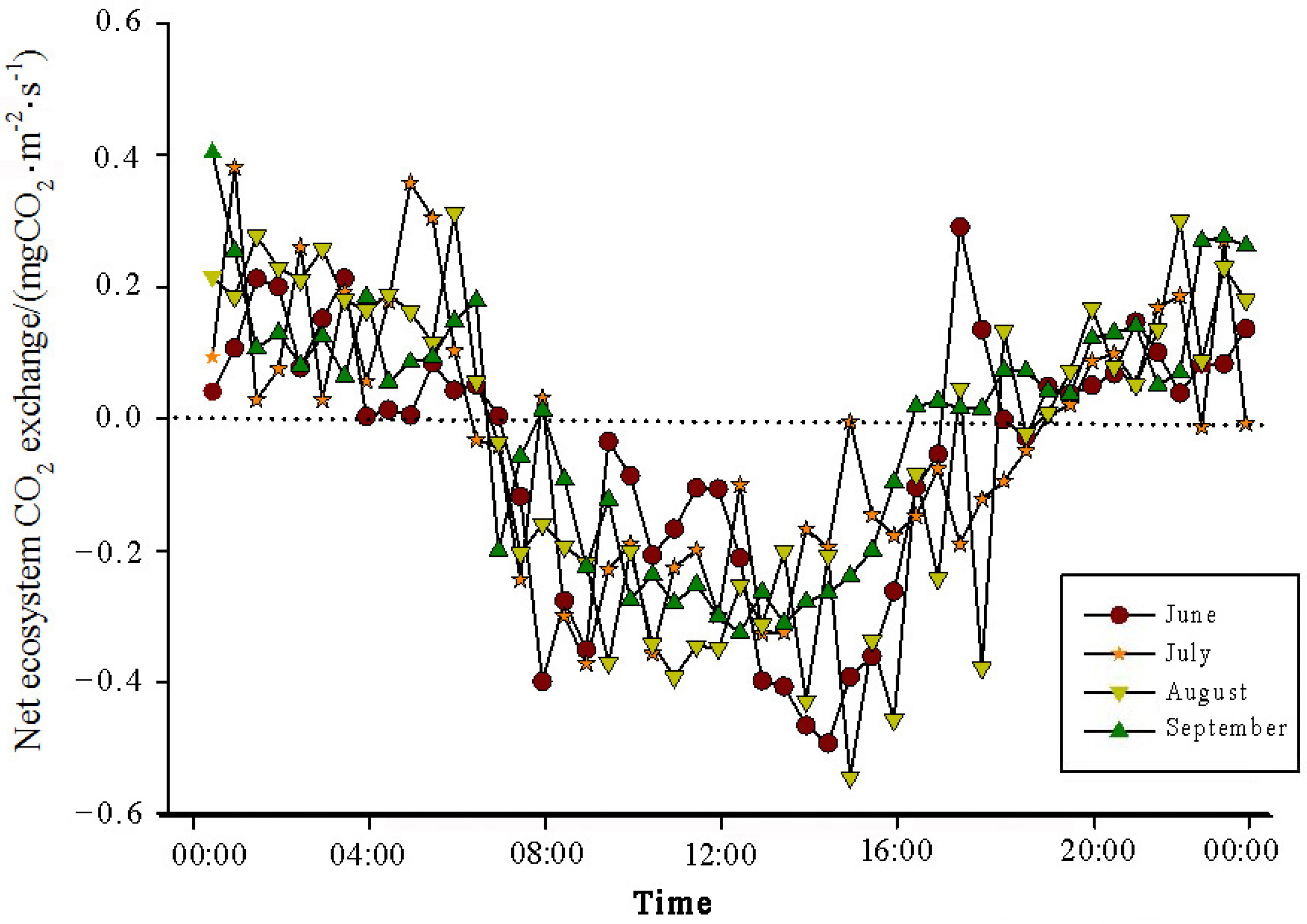
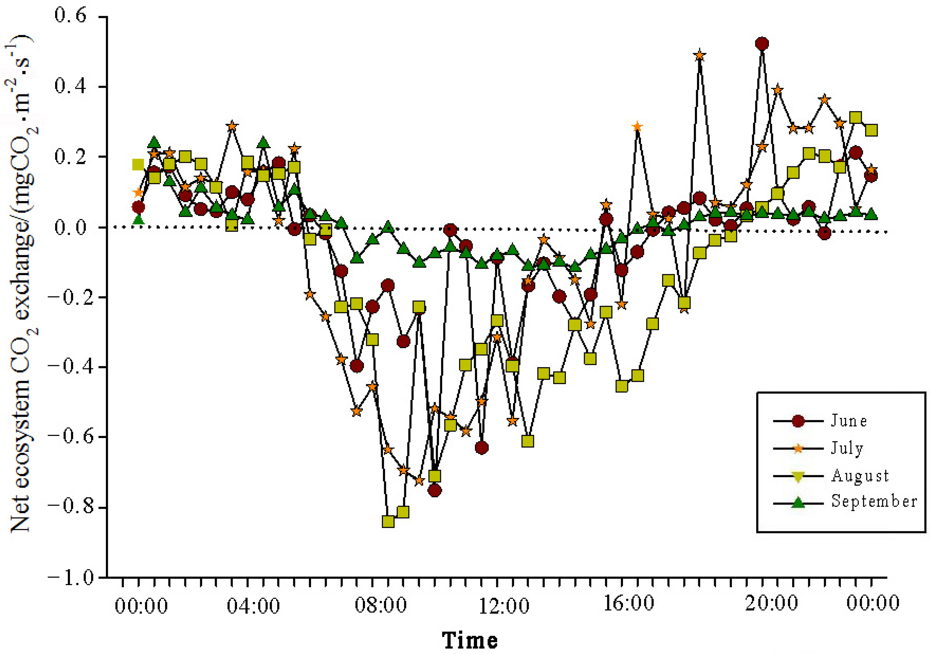
3.1. Daily Dynamics of Net CO₂ Exchange in the Salt Marsh Ecosystem

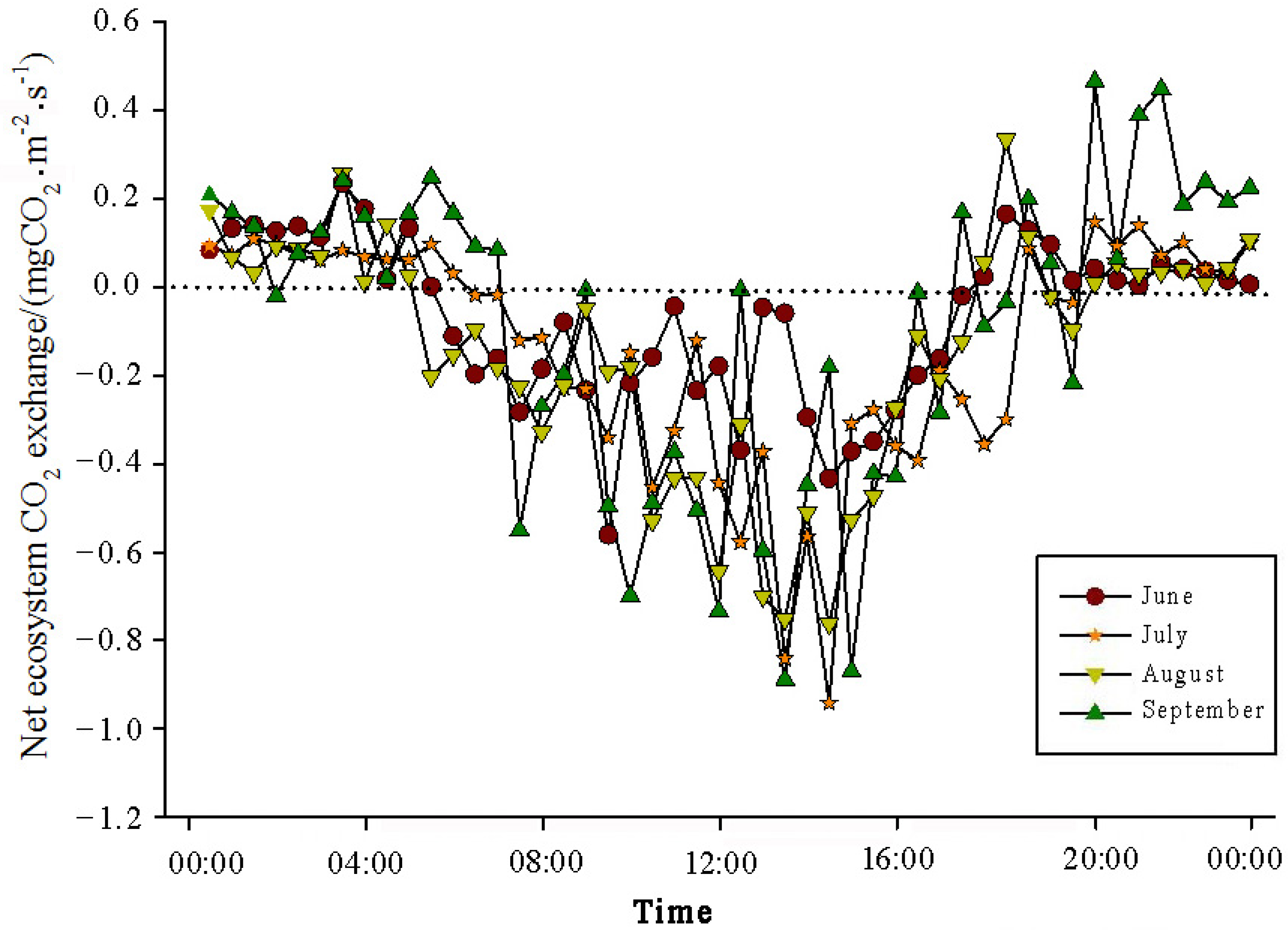
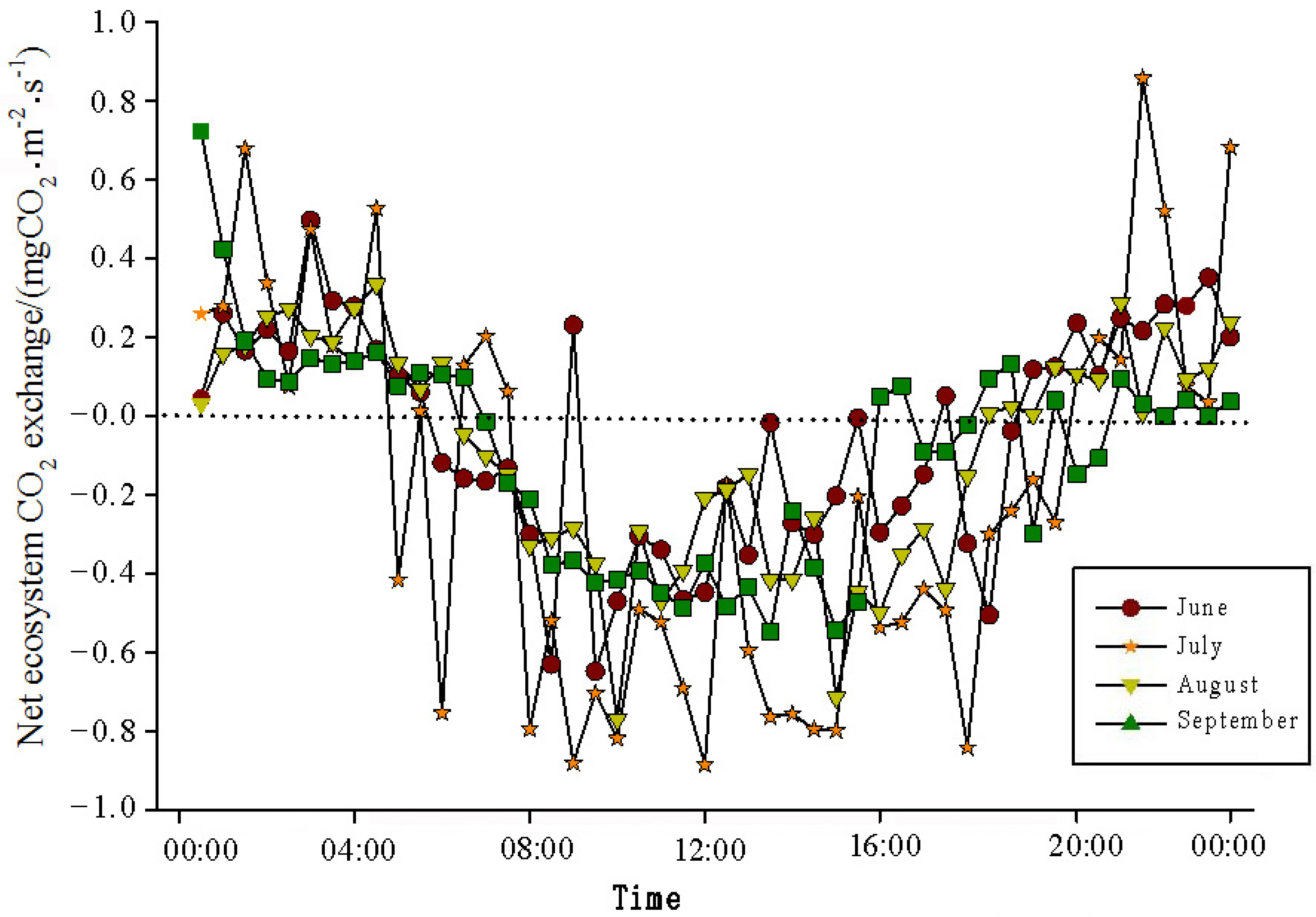
The analysis of the daily variations in CO₂ flux in the Momoge salt marsh ecosystem over four years during the growing season (June–September) showed two trends (Figure 3, Figure 4, Figure 5 and Figure 6). Throughout the day, the CO₂ flux in the Momoge salt marsh initially declined and subsequently increased. Prior to 6:00 AM, due to the respiration of wetland vegetation, the NEE was positive. After sunrise, around 7:00 AM, reeds initiated photosynthesis, which was stronger than the sum of the autotrophic respiration and heterotrophic respiration of reeds and soils, resulting in carbon uptake. This uptake intensity increased with enhanced solar radiation. From 8:00 AM to 11:00 AM, the carbon uptake rate reached its peak. In the first trend, during the midday period from 11:00 AM to 1:00 PM, carbon uptake diminished due to light saturation, a phenomenon often referred to as midday depression. Around 4:00 PM in the afternoon, the ecosystem’s carbon sequestration capacity started to increase again, reaching the second peak of CO₂ uptake (Figure 3 and Figure 5). Subsequently, the carbon uptake gradually decreased. Around 5:00 PM, the net carbon exchange shifted from negative to positive values, with NEE approaching zero. During this time, the vegetation mainly engaged in respiration, releasing CO₂. The ecosystem began to emit CO₂ to the atmosphere, and photosynthesis essentially ceased. In the second trend, the ecosystem only had one uptake peak (Figure 4) from 12:00 PM to 1:00 PM. After reaching the absorption peak around 12:00 PM, the absorption was suppressed in the afternoon due to light saturation. The amount of absorbed CO₂ began to decrease, and the rate of carbon sequestration in the ecosystem declined gradually. From approximately 7:00 PM to 8:00 PM, the ecosystem became a CO₂ source.

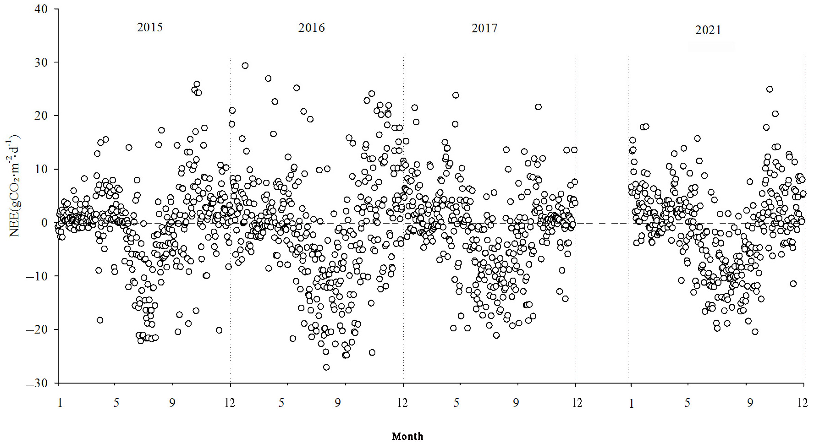
3.2. Seasonal and Interannual Dynamics of Net CO₂ Exchange

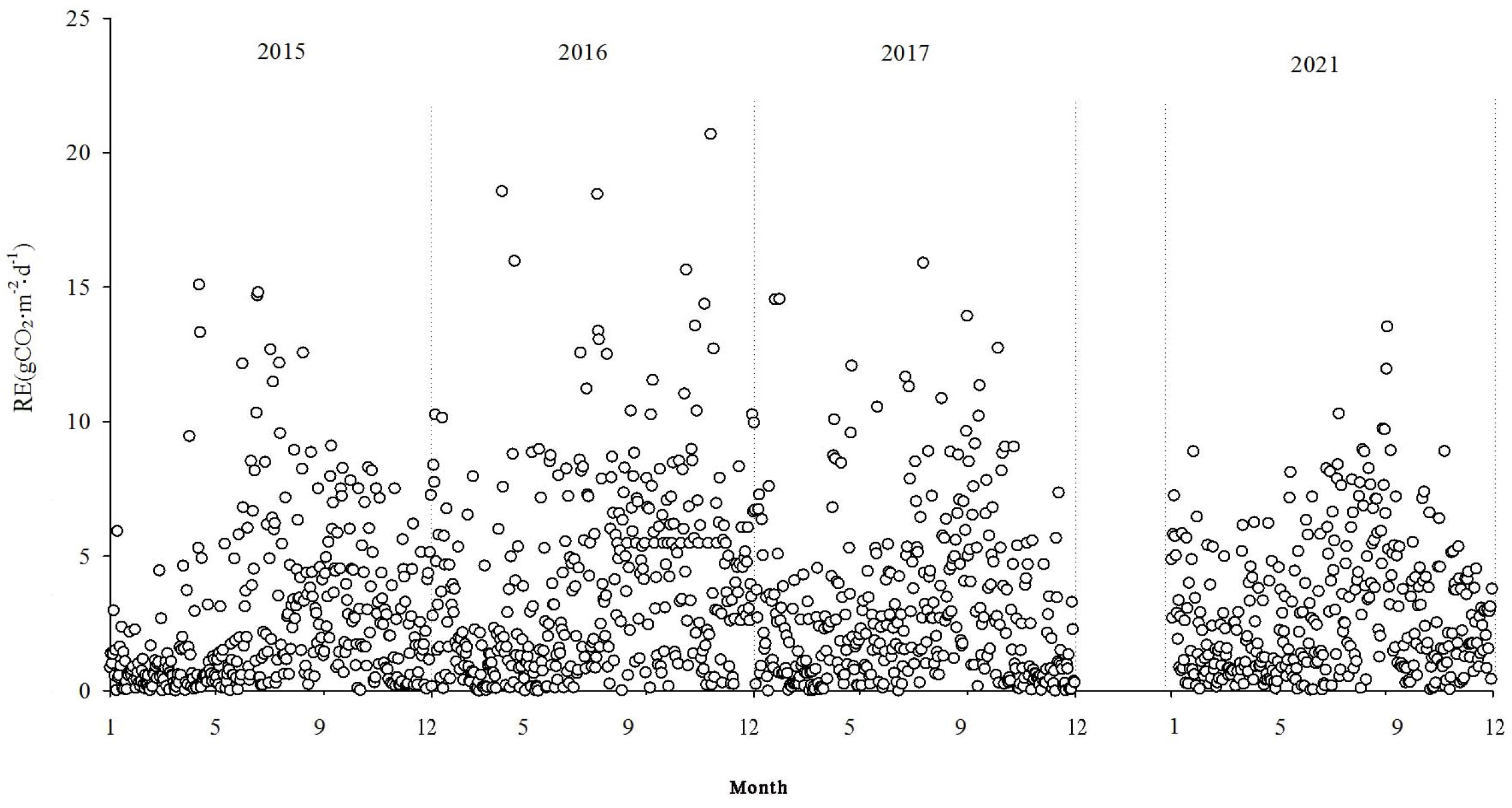
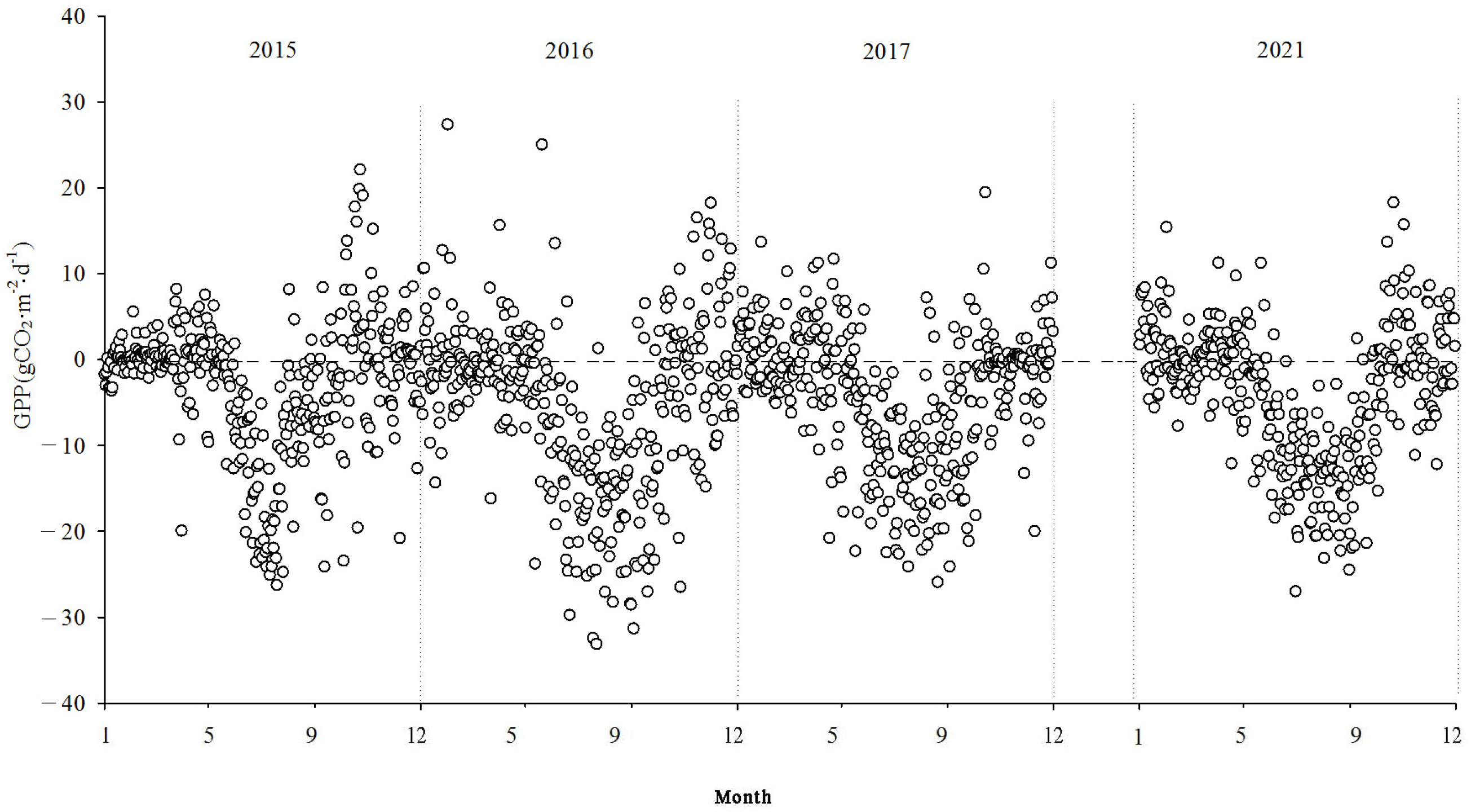
Figure 7, Figure 8 and Figure 9 show the interannual dynamics of different components of CO₂ fluxes in the Momoge salt marsh from 2015 to 2017 and in 2021, where the NEE, GPP, and ecosystem respiration (Reco) are daily cumulative values (g CO₂·m⁻²·d⁻¹). The GPP and Reco were estimated using the NEE.

During the study period, the NEE values illustrated the variations in carbon source/sink dynamics within the study area. Each year, the variation in carbon flux in the study area approximately followed a “V” shape. During the non-growing seasons, the carbon flux tended to be positive, indicating CO₂ emissions into the atmosphere. The Momoge salt marsh ecosystem acted as a CO₂ source. During the growing season, the carbon flux was predominantly negative, indicating the absorption of CO₂ from the atmosphere. The Momoge salt marsh functioned as a carbon sink during this period. Throughout the observation period, the average daily cumulative NEE value was approximately −1.03 g CO₂·m⁻²·d⁻¹. The numbers of days with negative carbon flux were 163, 202, 193, and 186 in 2015, 2016, 2017, and 2021, respectively. The proportion of negative carbon flux days was 51% for the entire observation period. During the high vegetation growth period in summer, the carbon flux values could be relatively high, even reaching positive values. This situation was typically observed during rainy or cloudy days between June and September. Due to the low PAR under such conditions, the NEE values generally tended to be small. With weaker vegetation photosynthesis and elevated temperatures, ecosystem respiration intensified, resulting in the wetland ecosystem acting as a carbon source.

At the interannual scale, the monthly mean daily dynamics of NEE exhibited a characteristic “V”-shaped curve, showing significant variations across seasons. During the non-growing season, the overall fluctuations were relatively small, whereas during the growing season, the overall fluctuations were more pronounced.

Reco encompasses both soil and plant respiration. During the non-growing season, the Reco values were relatively low but still positive, indicating the emission of CO₂ into the atmosphere. As temperatures rose, Reco gradually increased, reaching its peak during the summer months. During the study period, Reco values varied within the range of 0.002 g CO₂·m⁻²·d⁻¹–20.702 g CO₂·m⁻²·d⁻¹, with a mean value of 3.08 g CO₂·m⁻²·d⁻¹.

The total GPP of the ecosystem exhibited a yearly “V”-shaped pattern. During the non-growing season, the GPP values were relatively low. In the early growing season, with the emergence of reeds and the increase in leaf area, both the GPP and Reco started to rise. As the vegetation’s physiological activities intensified and photosynthesis dominated respiration, the wetland ecosystem acted as a carbon sink. During the main growing period (June to September), the GPP and Reco grew gradually.

3.3. Ecosystem CO₂ Balances

The dynamics of ecosystem CO₂ exchange were closely linked to climate conditions and vegetation, displaying significant seasonal and interannual variations. The ecosystem acted as a carbon sink during the growing season (May–October) and as a carbon source during the non-growing season (December–April) (Figure 10).

The four distinct seasons of the climatic conditions and vegetation in the Momoge salt marsh led to noticeable variations in the CO₂ flux of the wetland ecosystem. This could be observed in the average daily data for each month. By calculating the daily average CO₂ flux for each month from 2015 to 2017 and in 2021, a monthly average CO₂ flux graph was generated. As shown in Figure 8, the monthly average CO₂ flux was positive from January to April and from October to December. This indicates that the ecosystem emitted CO₂ to the atmosphere, acting as a carbon source. In May, as reeds started to sprout, photosynthesis intensified and the amount of CO₂ absorbed by reeds gradually increased. From June to September, the wetland entered its growing season, and the monthly average carbon flux values were negative. July marked the peak, where the ecosystem absorbed CO₂ from the atmosphere. During this period, the reed wetlands exhibited significant carbon sink activity during the day. Subsequently, as the reeds entered the senescence phase, the amount of absorbed CO₂ decreased, and the system shifted back to emitting carbon. Overall, within the study period, the wetland ecosystem exhibited its strongest carbon sequestration capacity in July, with a minimum monthly cumulative carbon flux of up to −359.98 g CO₂·m⁻² (July 2021). On the other hand, the month of January had the highest carbon emissions to the atmosphere, with a maximum monthly cumulative carbon flux of 185.89 g CO₂·m⁻² (October 2015). The CO₂ flux differed significantly among the different months in each year, with the CO₂ flux values from June to September notably lower than those in the other months (F = 29.79, p < 0.001).

The NEE monitoring over the four years in the Momoge salt marsh revealed that it functions as a carbon sink overall. The carbon sequestration intensities for each year were as follows: 206.94 g CO₂·m⁻²·yr⁻¹, 500.28 g CO₂·m⁻²·yr⁻¹, 436.88 g CO₂·m⁻²·yr⁻¹, and 358.61 g CO₂·m⁻²·yr⁻¹ in 2015, 2016, 2017, and 2021, respectively. The cumulative GPP values were −1152.62 g CO₂·m⁻²·yr⁻¹, −1928.62 g CO₂·m⁻²·yr⁻¹, −1516.79 g CO₂·m⁻²·yr⁻¹, and −1409.74 g CO₂·m⁻²·yr⁻¹. The cumulative Reco values were 945.68 g CO₂·m⁻²·yr⁻¹, 1428.34 g CO₂·m⁻²·yr⁻¹, 1079.91 g CO₂·m⁻²·yr⁻¹, and 1051.13 g CO₂·m⁻²·yr⁻¹, respectively.

3.4. Effects of Environmental Factors on CO₂ Exchange in the Wetland Ecosystem

3.4.1. Daily Scale

Pearson correlations were used to analyze the correlations between the factors and the dependent variable. A matrix of the correlation coefficients between the independent variables is shown in

Table 1. Pearson’s correlation coefficients for effects at the daily scale.

	NEE	Tsoil	Tair	PAR	PPT	WL
NEE	1	−0.488 ***	−0.452 ***	−0.327 ***	−0.182 **	0.463 ***
Tsoil	-	1	0.932 ***	0.564 ***	0.136 **	−0.914 ***
Tair	-	-	1	0.667 ***	0.153 **	−0.901 ***
PAR	-	-	-	1	−0.022	−0.603 ***
PPT	-	-	-	-	1	−0.076
WL	-	-	-	-	-	1

Note: ** represents a significance level of p < 0.01; *** represents a significance level of p < 0.001. NEE, net ecosystem exchange; PAR, photosynthetically active radiation; PPT, daily precipitation; Tair, air temperature; Tsoil, soil temperature; WL, water level.

. NEE represents the daily average CO₂ exchange, Tsoil represents the temperature at a soil depth of 5 cm at the daily scale, Tair represents the daily average air temperature, PAR represents the daily average photosynthetically active radiation, PPT represents the daily precipitation, and WL represents the water level.

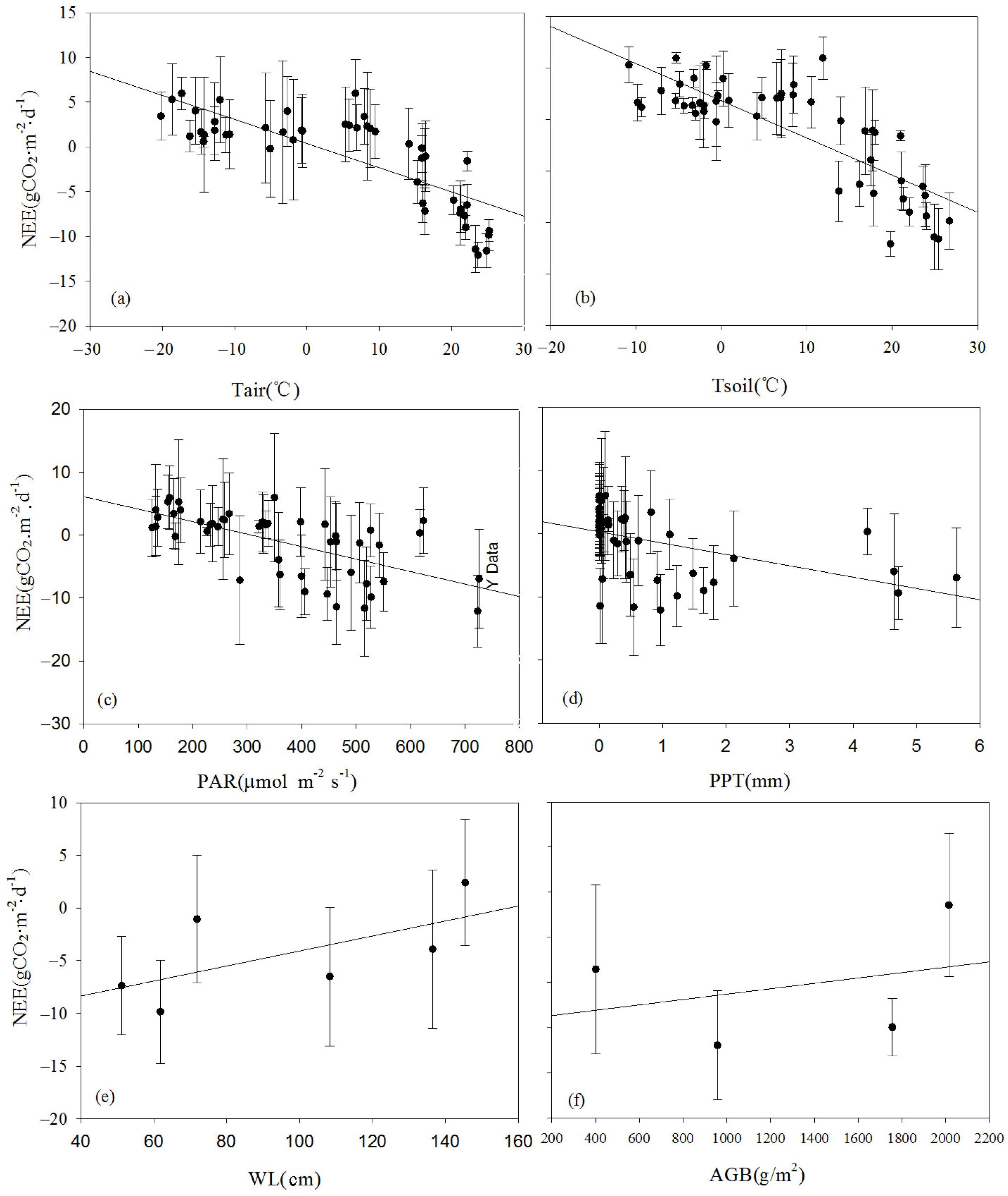
From the table, the Tsoil, PAR, PPT, and WL all significantly influenced the net CO₂ exchange. Specifically, the Tair, Tsoil, and PAR exhibited negative correlations with net CO₂ exchange. As the temperature and PAR increased, the net CO₂ exchange of the ecosystem decreased, indicating a trend towards an enhanced carbon absorption capacity. The PPT was negatively correlated with the net CO₂ exchange. On rainy days, lower solar radiation resulted in reduced CO₂ absorption. The WL showed a positive correlation with the net CO₂ exchange. As the WL rose, the proportion of plants exposed to the surface decreased, leading to a reduction in the wetland’s carbon absorption capacity.

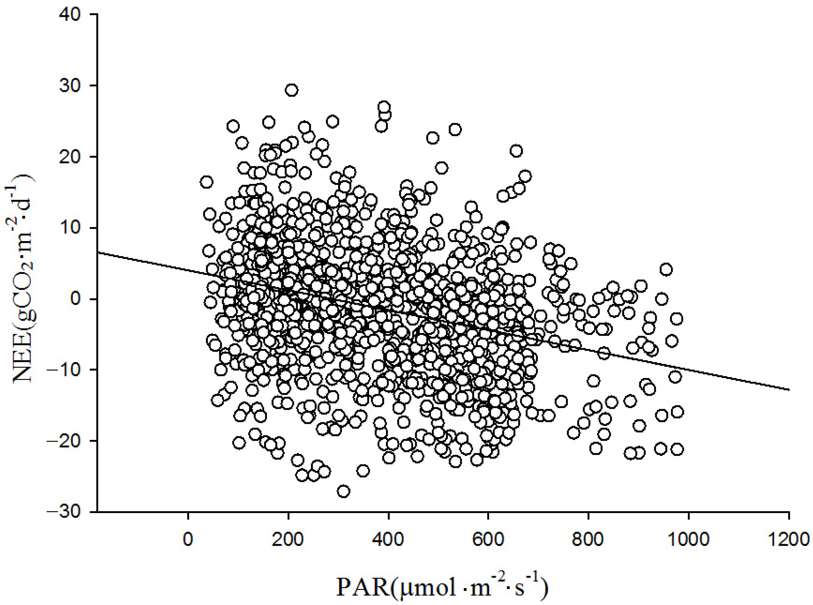
The role of PAR on the net exchange of CO₂ in wetlands was mainly reflected in the daytime of the growing season. In Figure 11, the net CO₂ exchange evidently increased rapidly with the rise in PAR. However, as the PAR intensity surpassed a certain threshold, the rate of the increase in the net CO₂ exchange slowed, eventually reaching a steady-state value. The influence of PAR was highly significant during different growth stages of the reeds. The phenomenon of net CO₂ absorption was closely related to the growth activities of the reeds. During the sprouting to flowering period from 4 May to 18 August, the wetland exhibited a strong photosynthetic assimilation capacity, with the maximum carbon absorption reaching up to 1.9 mg·m⁻²·s⁻¹. During the early and late stages of reed growth, the carbon absorption capacity was relatively weak, with the maximum carbon absorption reaching only 0.94 mg·m⁻²·s⁻¹.

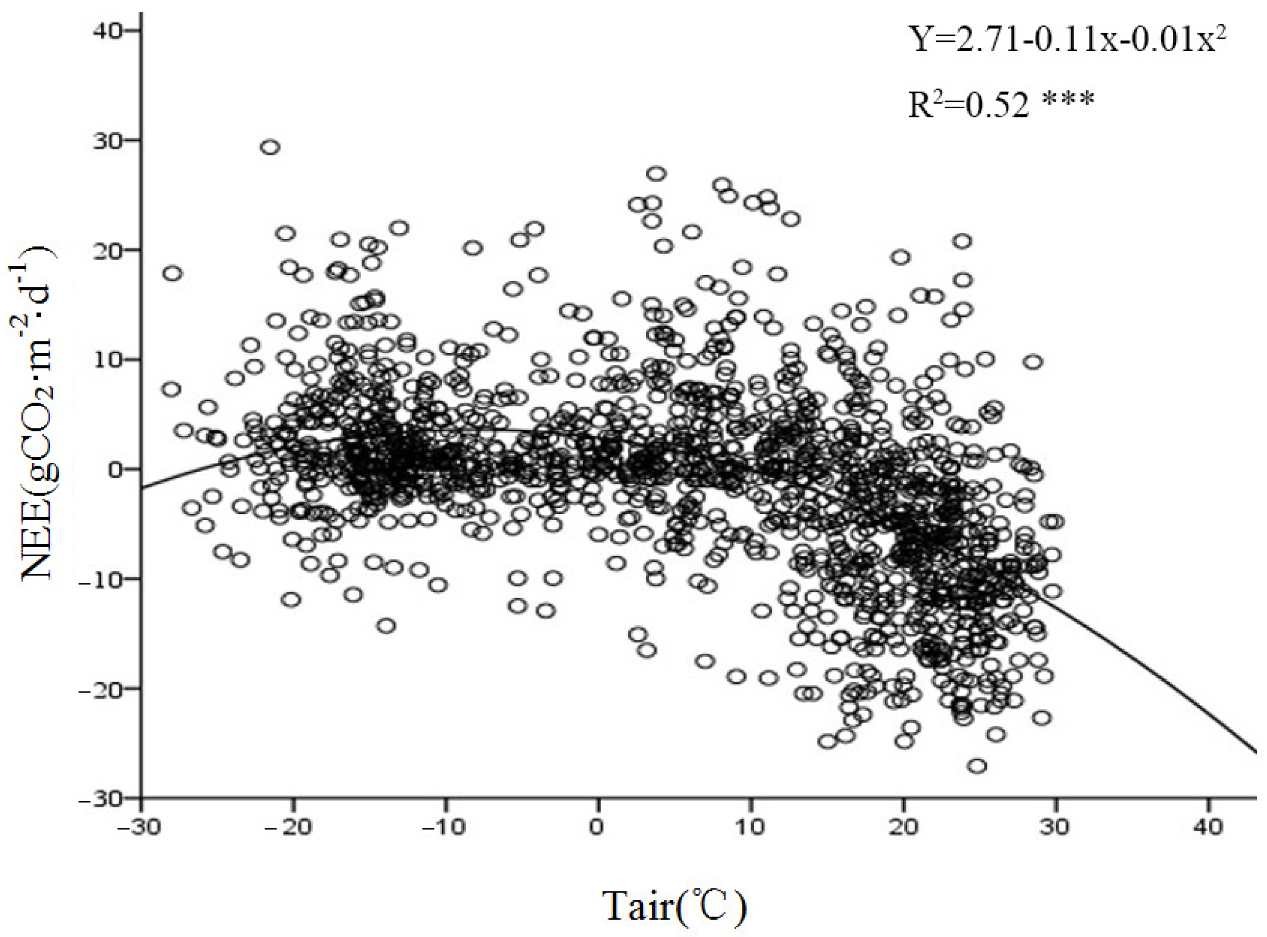
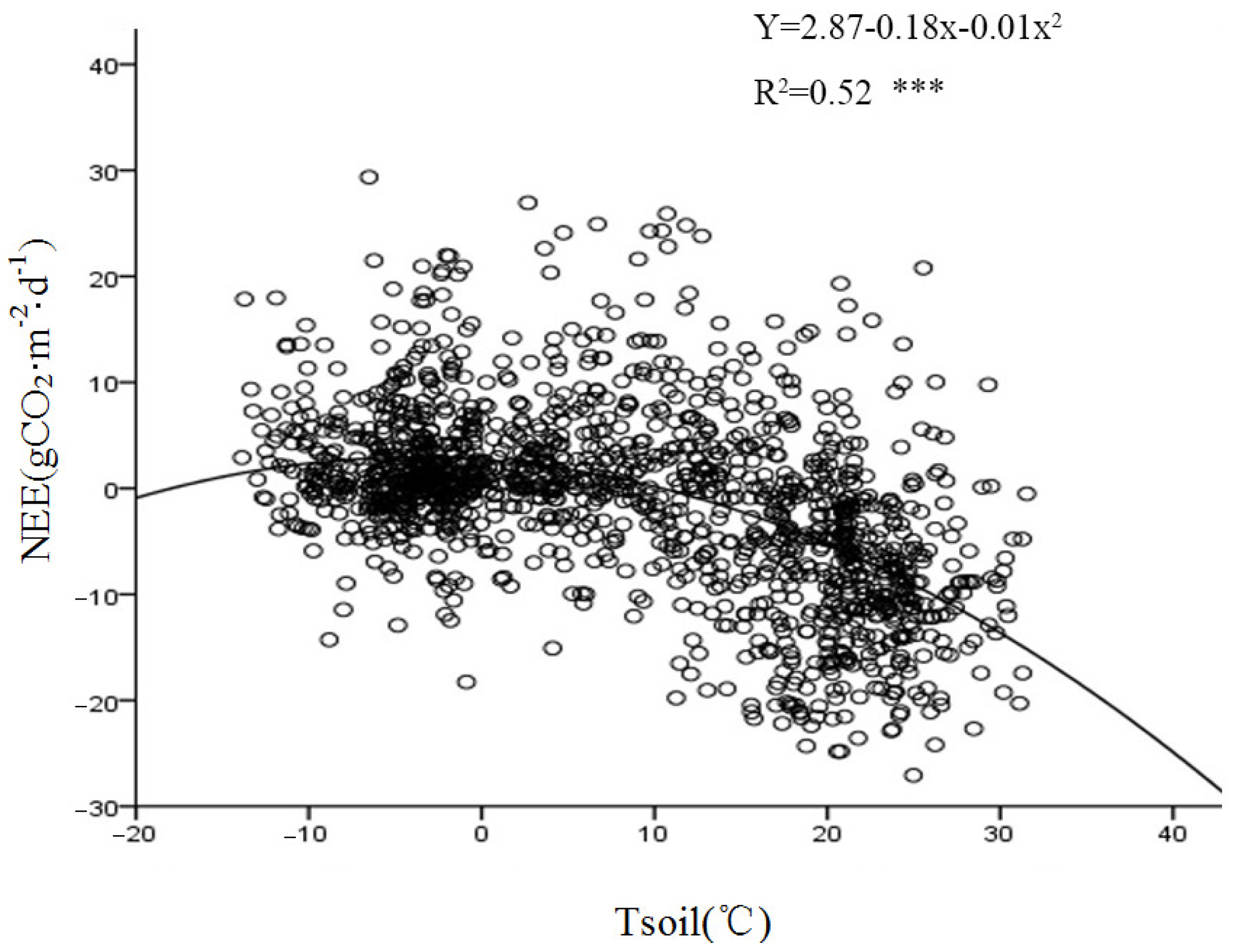
The temperature during the growing season had a significant impact on the photosynthetic physiology of the vegetation and was the most important meteorological factor affecting the respiration intensities of various components within the ecosystem. Figure 12 demonstrates a significant exponential correlation between the nighttime CO₂ flux and Tsoil at a depth of 5 cm. A comparative analysis of the relationship between the nighttime carbon flux and the 2.5 m air temperature during the growing and non-growing seasons (Figure 13) revealed an exponential growth trend in the response of the nighttime carbon flux to Tair. This suggests that the intensity of nighttime carbon release is directly controlled by thermal conditions. Both Tair and the upper Tsoil affected the respiration rate of the ecosystem. An increase in temperature accelerated the metabolism of plants and microorganisms, thus enhancing the intensity of carbon emissions.

3.4.2. Seasonal Scale

The effects of environmental control variables (Tair, Tsoil, PAR, PPT, WL, and AGB) on NEE are often complex and interrelated. To investigate the mechanisms influencing NEE, a correlation analysis was conducted between the monthly average NEE and the environmental factors at the seasonal scale (

Table 2. Pearson’s correlation coefficients for effects at the monthly scale.

	NEE	Tsoil	Tair	PAR	PPT	WL	AGB
NEE	1	−0.811 ***	−0.783 ***	−0.629 ***	0.476 ***	0.635	−0.469 *
Tsoil	-	1	0.950 ***	0.676 ***	0.436 **	−0.741	0.104
Tair	-	-	1	0.812 ***	0.525 ***	−0.737	−0.068
PAR	-	-	-	1	0.545 ***	−0.969 ***	0.904 *
PPT	-	-	-	-	1	0.030	0.042
WL	-	-	-	-	-	1	0.154
AGB							1

Note: * represents a significance level of p < 0.05; ** represents a significance level of p < 0.01; *** represents a significance level of p < 0.001. AGB, aboveground biomass; NEE, net ecosystem exchange; PAR, photosynthetically active radiation; PPT, daily precipitation; Tair, air temperature; Tsoil, soil temperature; WL, water level.

). Apart from the WL, significant linear correlations between the monthly average NEE and the main environmental and biological factors were found (Figure 14). They could be ranked in decreasing order of significance as follows: Tsoil > Tair > PAR > PPT > biomass (AGB). Larger values of Tsoil, Tair, PAR, and AGB indicated a stronger carbon uptake capacity of the ecosystem. Tair significantly influenced Tsoil, indicating that Tair indirectly affected NEE flux by influencing Tsoil. Concurrently, the monthly carbon uptake capacity significantly increased with an increase in Tair. The dynamics of AGB were more dependent on the variations in PAR. This was primarily because the monitoring area experienced prolonged waterlogged conditions, where the anaerobic environment inhibited the decomposition of detritus, leading to the accumulation of organic matter in the soil. As a result, the wetland became a carbon sink that suppressed the increase in the atmospheric CO₂ concentration. The impact of rainfall on biomass accumulation was relatively weak. Under waterlogged conditions, the reed biomass was relatively high, with the maximum biomass reaching up to 2.5 kg·m⁻². The plant height could exceed 270 cm, and the ground cover density was relatively high.

4. Discussion

Different wetland ecosystems exhibit varying net ecosystem CO₂ exchange rates across different time scales. Similarly, CO₂ exchange rates differ among wetland types. Even within the same wetland type, interannual CO₂ exchange varies notably. Currently, wetlands generally act as carbon sinks, with an average carbon sequestration rate of 118 gC·m⁻²·yr⁻¹ [7]. Numerous studies have indicated that reed wetlands and peatlands are significant carbon sinks [15]. Our study confirmed this by indicating that the Momoge salt marsh acted as a carbon sink in the years 2015–2017 and 2021. A study monitoring the NEE in the reed wetland of the Liaohe Delta in 2006 showed that this area also acted as a carbon sink, with a carbon sequestration intensity of 230 g CO₂·m⁻²·yr⁻¹ [16]. In the Nanji wetland of Poyang Lake, during the non-flooded period of 2015, the ecosystem acted as a carbon sink with a carbon sequestration rate of 667.62 g C·m⁻²·yr⁻¹. However, in the subsequent years of 2016 and 2017, it shifted to a carbon source [17]. A study of CO₂ fluxes for the entire year of 2005 in the Haibei wetland of the Qinghai–Tibet Plateau showed that it released around 86.18 g C·m⁻²·yr⁻¹ into the atmosphere, making it a carbon source as well [18]. The interannual variations in NEE in wetland ecosystems are closely linked to climate [19,20,21], hydrology [22], and vegetation conditions [23]. These factors collectively play a significant role in shaping the carbon sink functions of specific ecosystems. Furthermore, related studies have indicated that even within the same wetland ecosystem, the carbon source/sink status can exhibit uncertainty across interannual periods due to variations in vegetation composition, hydrological conditions, human disturbances, and climate change [24]. Since wetland greenhouse gas balances are highly sensitive to changes in wetland area, the future impact of wetlands on the climate depends on the balance between degradation and restoration.

This study found that the NEE of wetlands exhibited a pattern of functioning as a carbon sink with greater fluctuations during the growing season and as a carbon source with smaller fluctuations during the non-growing season. During the spring, as plants start sprouting and growing, the amount of carbon fixed through photosynthesis is initially less than the carbon released through respiration. As a result, the wetland continues to act as a carbon source. However, as plant growth progresses and photosynthesis becomes stronger than respiration, the wetland transitions to a carbon sink. Along with the peak of plant growth, the maximum values of NEE typically occur in July and August. Subsequently, as temperatures decrease and plants enter their senescence phase, their photosynthetic capacity gradually diminishes. This reduction in photosynthesis leads to a significant decrease in the NEE. This pattern is consistent with findings from previous research [25]. By November, the wetland vegetation is completely withered. Due to ecosystem respiration, the wetland transitions entirely to functioning as a carbon source.

A significant amount of research has indicated that when the solar radiation intensity is low, net CO₂ exchange increases with the increase in PAR, following a hyperbolic trend. Many studies have shown a significant correlation between NEE and PAR. Ecosystems such as forests, grasslands, and croplands exhibit a positive relationship between solar radiation intensity and net carbon exchange, following a hyperbolic curve [26]. Similar conclusions were drawn by Beverland et al. [27] in the context of wetland ecosystems. The current study also revealed that in the reed wetland, the net CO₂ exchange initially increases rapidly with an increase in PAR. However, after PAR exceeds a certain threshold, the rate of the increase in the net CO₂ exchange slows, eventually converging to an asymptote value. The phenomenon of net CO₂ absorption is closely tied to the growth activities of reeds. Furthermore, related studies have shown that the response of NEE to solar radiation is also influenced by other limiting factors, such as the atmospheric vapor pressure deficit and occasionally frost [28,29]. The influence of the radiation intensity on the net CO₂ exchange is more pronounced within a suitable temperature range. Additionally, a larger leaf area index corresponds to a more distinct response of net CO₂ exchange to radiation intensity.

Most studies suggest that changes in WL and temperature increases can significantly affect the production of CO₂ in wetland ecosystems [30,31,32]. Research on wetlands in southern Finland found that a high temperature is the primary factor leading to an increase in net carbon uptake [33]. This study found that nighttime carbon flux exhibits an exponential growth trend in response to Tair. Temperature affects ecosystem CO₂ flux through both direct and indirect mechanisms, ultimately influencing ecological processes [34]. Firstly, the seasonal variation in photosynthesis is primarily controlled by temperature [35]. Within a certain temperature range, higher temperatures are more favorable for photosynthesis [36]. For example, studies on the seasonal cumulative GPP of corn and wheat ecosystems found that higher mean temperatures are associated with larger cumulative GPP values [37]. Research on temperate bulrush marshes also showed that temperature is a key indicator for daily GPP [38]. Furthermore, ecosystem respiration is primarily controlled by temperature, with respiration increasing exponentially as temperature rises [39]. This is because higher temperatures can stimulate dark respiration in both soil and vegetation. Research on northern marshes revealed that higher temperatures correspond to higher ecosystem respiration rates [40]. At both interannual and seasonal scales, the Reco of salt marshes was found to be significantly correlated with temperature [41]. Furthermore, CO₂ fluxes are controlled by temperature through its effects on vegetation cover, the leaf area index, and the length of the growing season. An increase in Tsoil is accompanied by an increase in AGB [42]. The temperature in the environment controls the humidity by regulating the vapor pressure. Research on wetlands in the southwestern plateau of China found that temperature can explain most of the seasonal variability in carbon fluxes. Warming can increase both GPP and Reco, thus influencing the carbon balance of the plateau wetlands [43]. Although water level conditions significantly influence the uptake and release of CO₂ in the ecosystem, temperature remains the primary factor for carbon fluxes in the Momoge salt marsh.

5. Conclusions

This study analyzed the CO₂ flux variation characteristics and the factors affecting them in the Momoge salt marsh ecosystem. During the growing season, we observed an initial decline and a subsequent increase in the daily variations in CO₂ fluxes in the Momoge salt marsh, with uptake occurring during the day (negative values) and release taking place at night (positive values). Two patterns emerged (one peak and two peaks), with reduced carbon absorption during midday due to light saturation resulting in a midday depression phenomenon for the latter pattern. Within each annual variation, the carbon fluxes in the study area roughly exhibited a “V” shape. The carbon fluxes during the non-growing season predominantly showed positive values, indicating the release of CO₂ into the atmosphere_. The carbon sequestration intensities of the Momoge salt marsh ecosystem were 206.94 g CO₂·m⁻²·yr⁻¹, 500.28 g CO₂·m⁻²·yr⁻¹, 436.00 g CO₂·m⁻²·yr⁻¹, and 358.61 g CO₂·m⁻²·yr⁻¹ for the years 2015–2017 and 2021, respectively. This indicates that the system behaves as a carbon sink.

At both the hourly and daily scales, PAR was the primary factor affecting daytime variations in NEE during the growing season, while temperature was the main factor influencing nighttime NEE dynamics. At the daily scale, Tair, Tsoil, PAR, PPT, and WL all showed significant effects on net CO₂ exchange. At the monthly scale, larger values of Tsoil, Tair, PAR, and AGB corresponded to a stronger carbon absorption capacity of the ecosystem. As the WL rose, the proportion of plants exposed to the surface decreased, leading to a reduction in the wetland’s carbon absorption capacity. Although the WL conditions significantly influenced the uptake and release of CO₂ in the ecosystem, temperature remained the primary factor for carbon fluxes in the Momoge salt marsh.