

Evaluating the Performance of the Generalized Linear Model (glm) R Package Using Single-Cell RNA-Sequencing Data


Abstract
:1. Introduction
2. Materials and Design of Experiment
2.1. Datasets
2.2. Evaluation Procedure
2.3. Code Repository
3. Results and Analysis
| Algorithm 1 The complete algorithm for testing glm using Conquer datasets. |
|
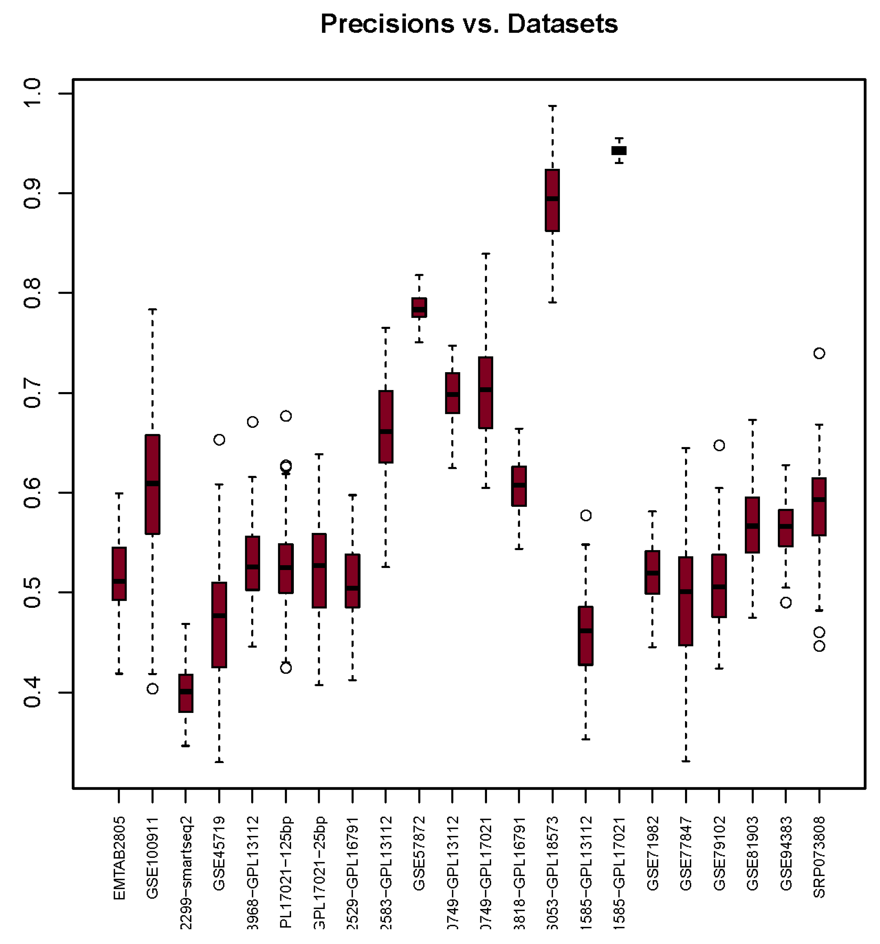
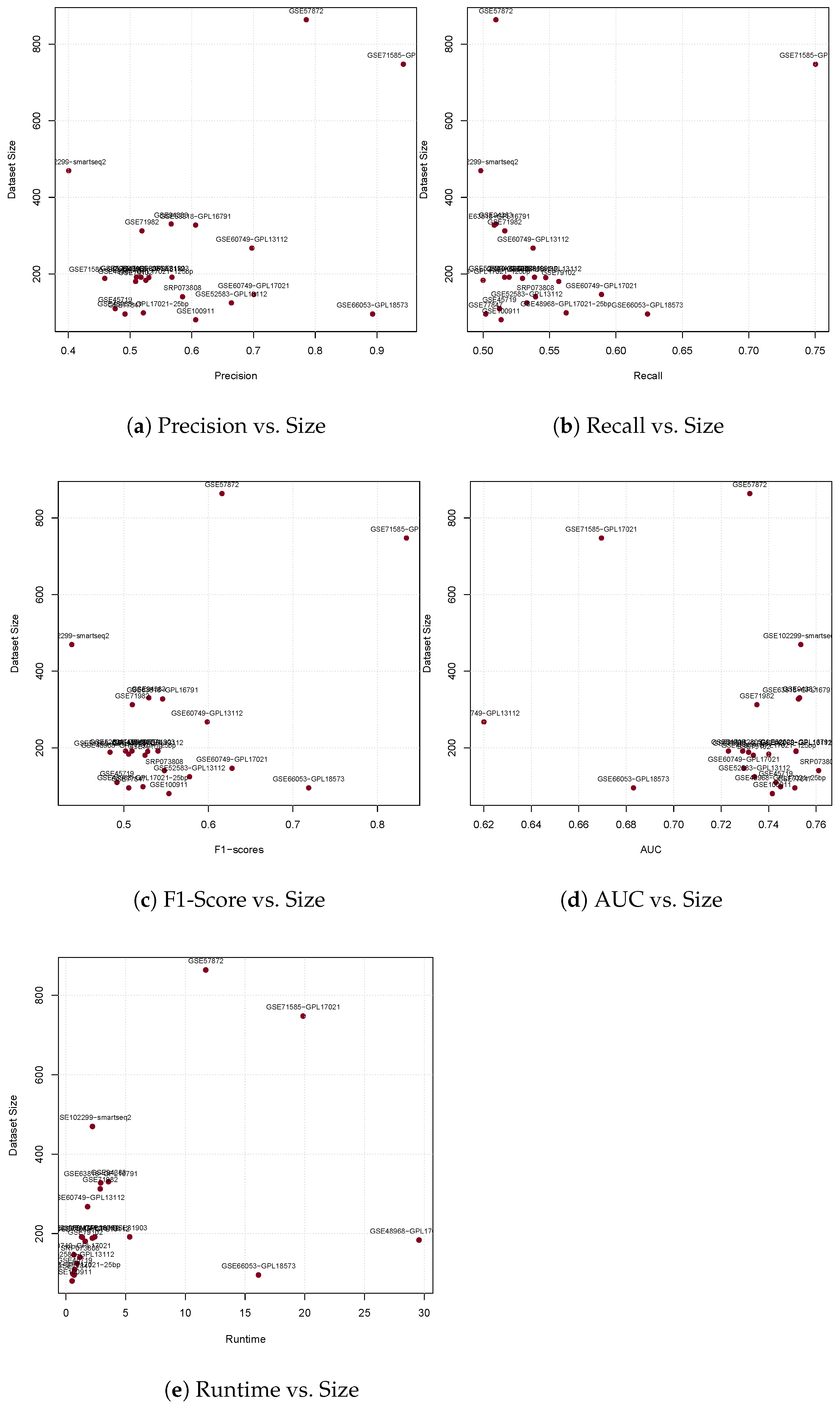
3.1. Precision
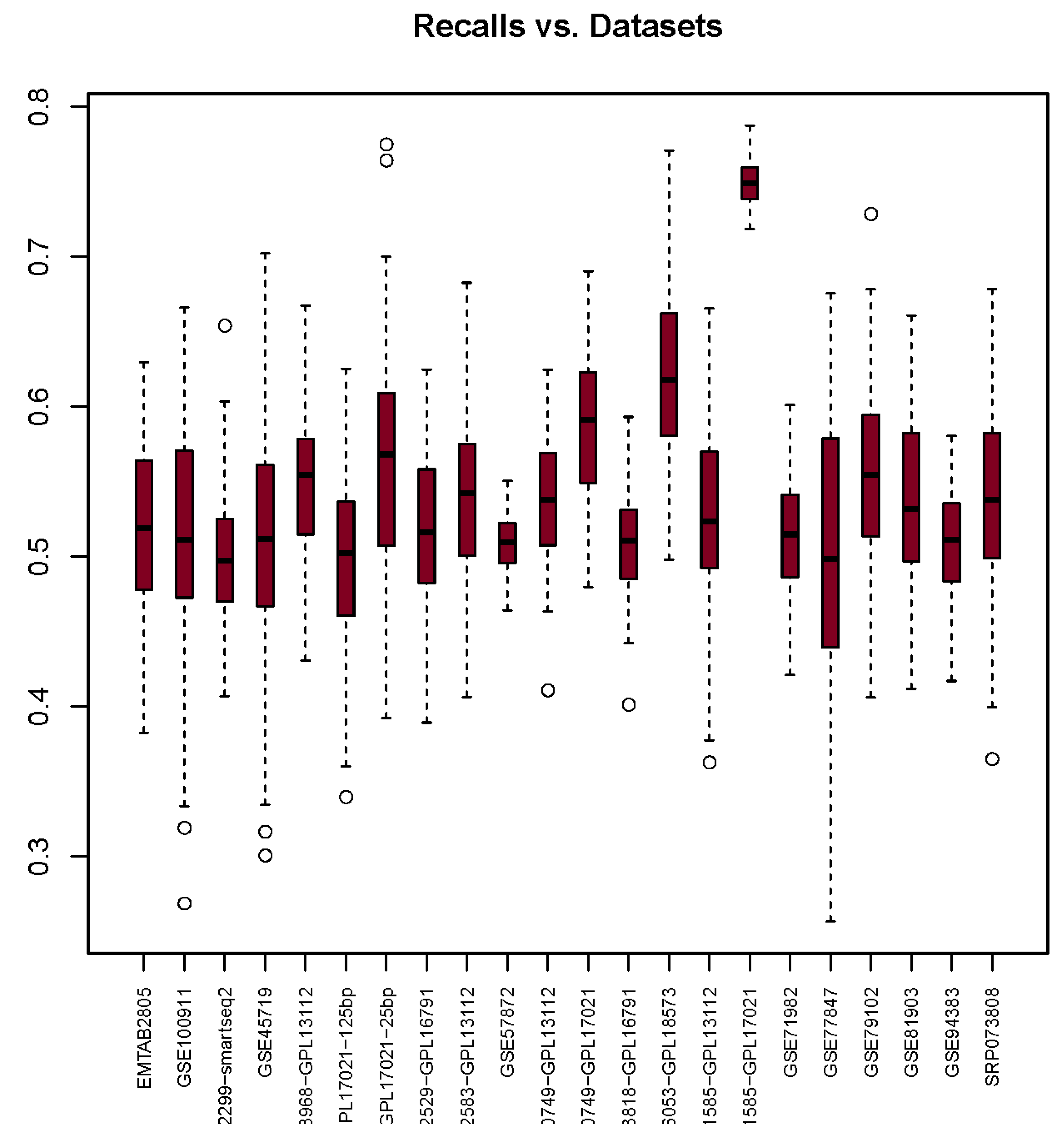
3.2. Recall
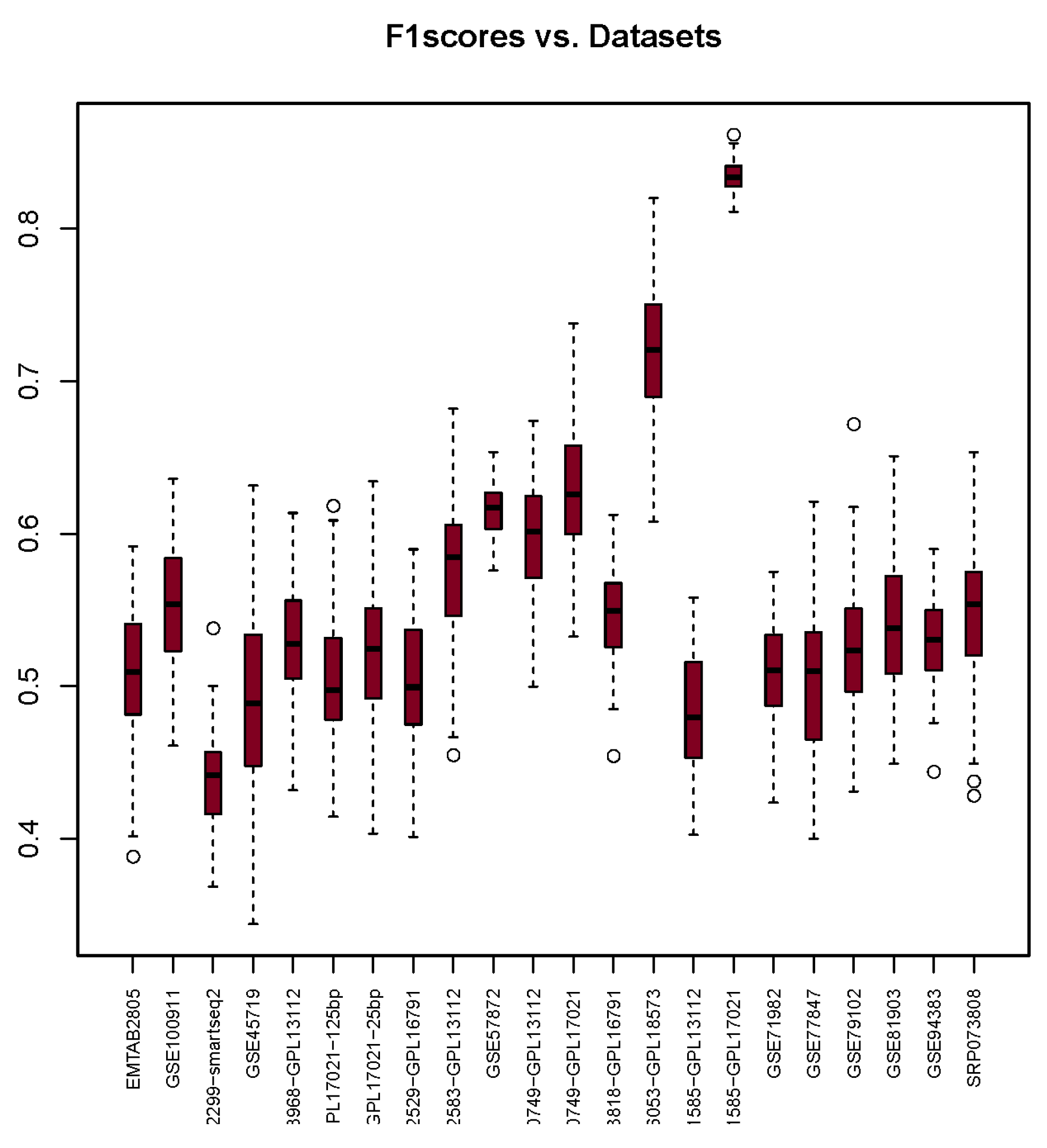
3.3. F1-Score
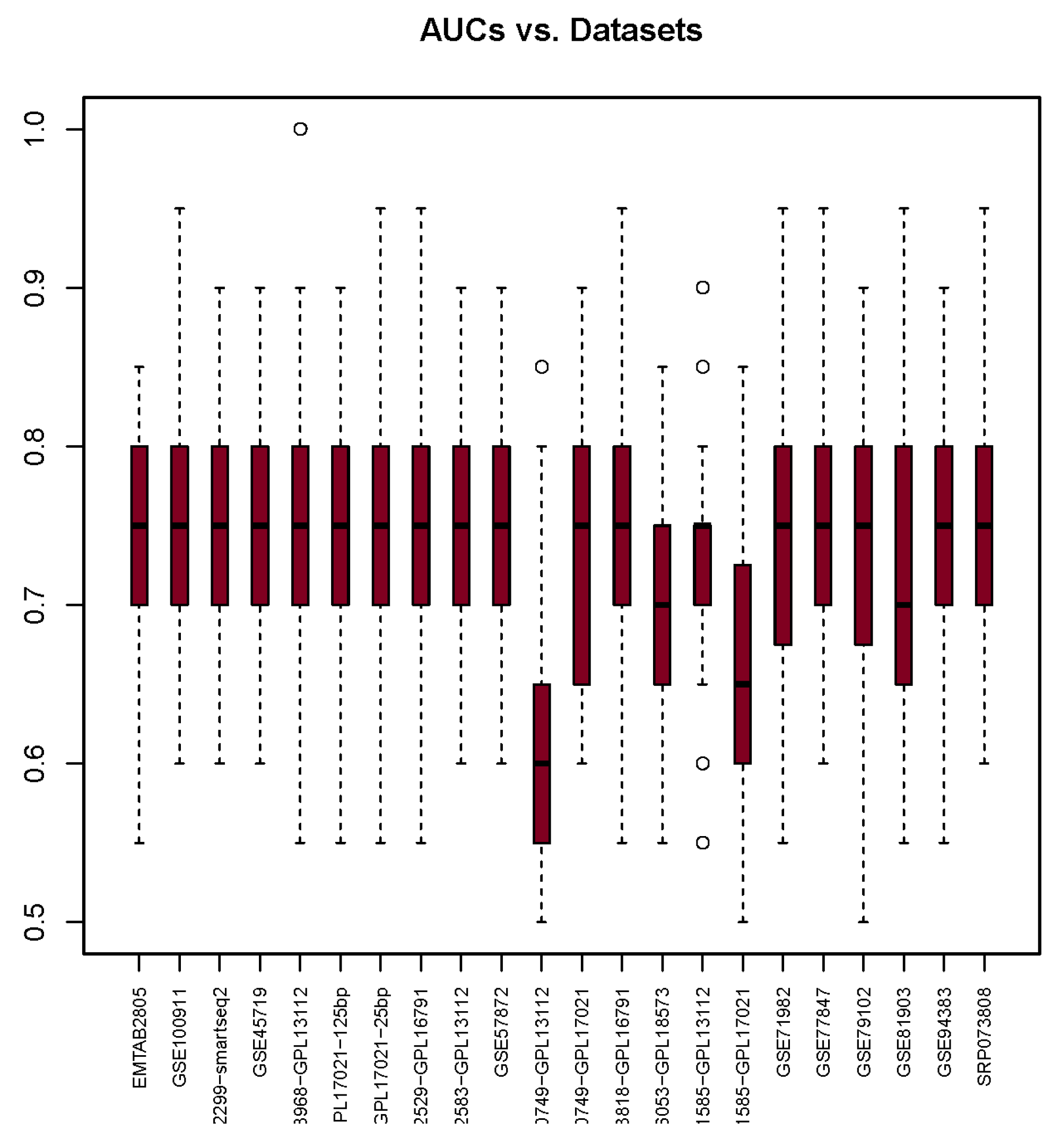
3.4. Area under the Curve
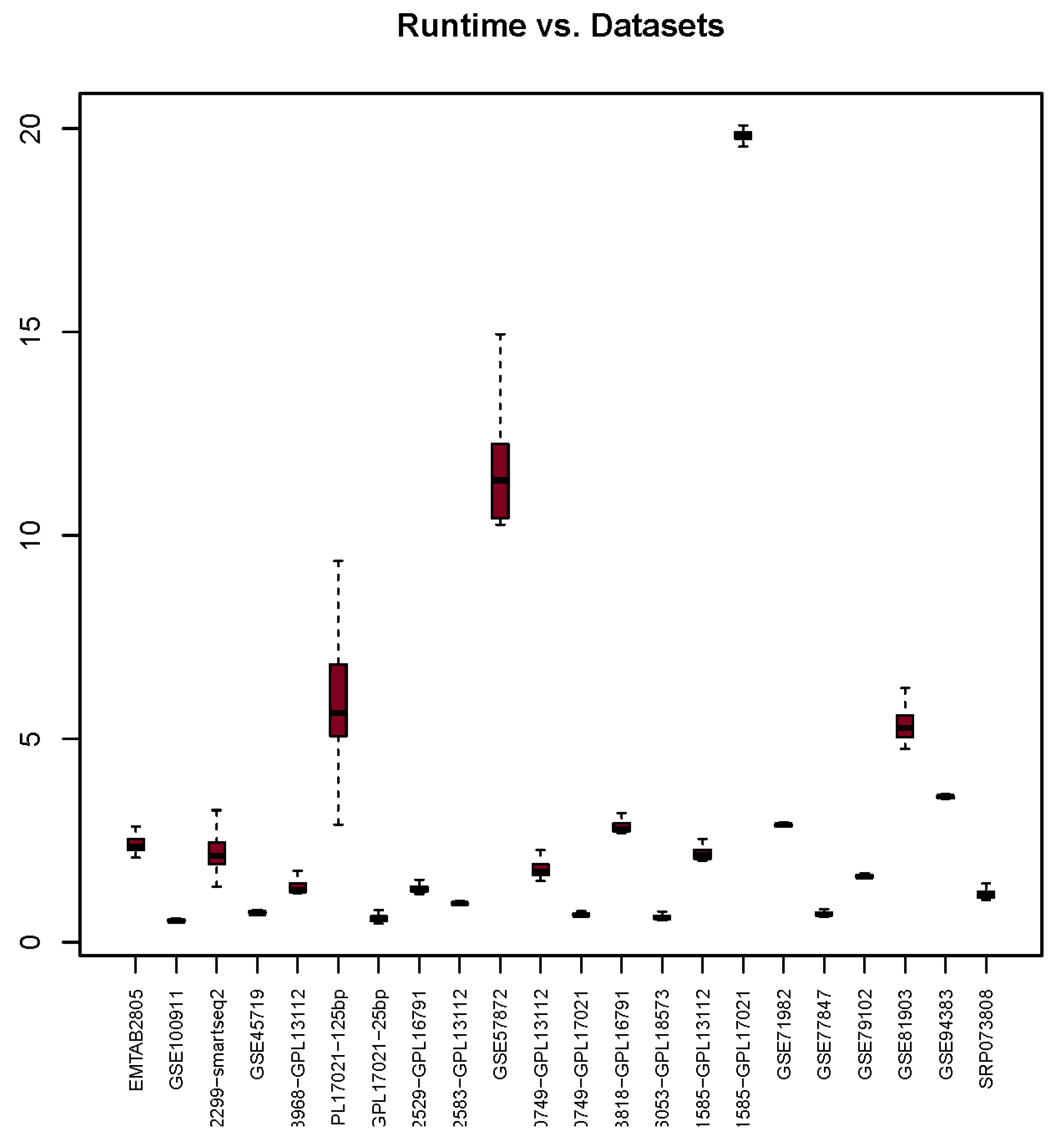
3.5. Runtime
4. Discussion and Conclusions
Author Contributions
Funding
Institutional Review Board Statement
Informed Consent Statement
Data Availability Statement
Conflicts of Interest
Abbreviations
| AUC | Area under the Curve |
| scRNA-seq | Single-cell Ribonucleic Acid Sequencing |
| ROC | Receiver Operating Characteristic |
References
- Cucchiara, A. Applied Logistic Regression. Technometrics 1992, 34, 358–359. [Google Scholar] [CrossRef]
- Dunn, P.K.; Smyth, G.K. Generalized Linear Models with Examples in R; Springer: Berlin/Heidelberg, Germany, 2018; Volume 53. [Google Scholar]
- Rutherford, A. ANOVA and ANCOVA: A GLM Approach; John Wiley & Sons: Hoboken, NJ, USA, 2011. [Google Scholar]
- Guisan, A.; Weiss, S.B.; Weiss, A.D. GLM versus CCA spatial modeling of plant species distribution. Plant Ecol. 1999, 143, 107–122. [Google Scholar] [CrossRef]
- Stefánsson, G. Analysis of groundfish survey abundance data: Combining the GLM and delta approaches. ICES J. Mar. Sci. 1996, 53, 577–588. [Google Scholar] [CrossRef]
- Pepe, M.S. An interpretation for the ROC curve and inference using GLM procedures. Biometrics 2000, 56, 352–359. [Google Scholar] [CrossRef]
- Tran, M.N.; Nguyen, N.; Nott, D.; Kohn, R. Bayesian deep net GLM and GLMM. J. Comput. Graph. Stat. 2020, 29, 97–113. [Google Scholar] [CrossRef]
- Potts, S.E.; Rose, K.A. Evaluation of GLM and GAM for estimating population indices from fishery independent surveys. Fish. Res. 2018, 208, 167–178. [Google Scholar] [CrossRef]
- Calcagno, V.; de Mazancourt, C. glmulti: An R Package for Easy Automated Model Selection with (Generalized) Linear Models. J. Stat. Softw. 2010, 34, 1–29. [Google Scholar] [CrossRef]
- Bi, J.; Kuesten, C. Type I error, testing power, and predicting precision based on the GLM and LM models for CATA data–Further discussion with M. Meyners and A. Hasted. Food Qual. Prefer. 2023, 106, 104806. [Google Scholar] [CrossRef]
- Xiong, Y. Building text hierarchical structure by using confusion matrix. In Proceedings of the 2012 5th International Conference on BioMedical Engineering and Informatics, Chongqing, China, 16–18 October 2012; pp. 1250–1254. [Google Scholar]
- Davis, J.; Goadrich, M. The relationship between Precision-Recall and ROC curves. In Proceedings of the 23rd International Conference on Machine Learning, Honolulu, HI, USA, 23–29 July 2006; pp. 233–240. [Google Scholar]
- Caelen, O. A Bayesian interpretation of the confusion matrix. Ann. Math. Artif. Intell. 2017, 81, 429–450. [Google Scholar] [CrossRef]
- Zhang, D.; Wang, J.; Zhao, X. Estimating the uncertainty of average F1 scores. In Proceedings of the 2015 International Conference on the Theory of Information Retrieval, Northampton, MA, USA, 27–30 September 2015; pp. 317–320. [Google Scholar]
- Zhang, D.; Wang, J.; Zhao, X.; Wang, X. A Bayesian hierarchical model for comparing average F1 scores. In Proceedings of the 2015 IEEE International Conference on Data Mining, Atlantic City, NJ, USA, 14–17 November 2015; pp. 589–598. [Google Scholar]
- Myerson, J.; Green, L.; Warusawitharana, M. Area under the curve as a measure of discounting. J. Exp. Anal. Behav. 2001, 76, 235–243. [Google Scholar] [CrossRef]
- Habermann, A.C.; Gutierrez, A.J.; Bui, L.T.; Yahn, S.L.; Winters, N.I.; Calvi, C.L.; Peter, L.; Chung, M.I.; Taylor, C.J.; Jetter, C.; et al. Single-cell RNA sequencing reveals profibrotic roles of distinct epithelial and mesenchymal lineages in pulmonary fibrosis. Sci. Adv. 2020, 6, eaba1972. [Google Scholar] [CrossRef] [PubMed]
- Bauer, S.; Nolte, L.; Reyes, M. Segmentation of brain tumor images based on atlas-registration combined with a Markov-Random-Field lesion growth model. In Proceedings of the 2011 IEEE International Symposium on Biomedical Imaging: From Nano to Macro, Chicago, IL, USA, 30 March–2 April 2011; pp. 2018–2021. [Google Scholar] [CrossRef]
- Pliner, H.A.; Shendure, J.; Trapnell, C. Supervised classification enables rapid annotation of cell atlases. Nat. Methods 2019, 16, 983–986. [Google Scholar] [CrossRef] [PubMed]
- Seyednasrollah, F.; Laiho, A.; Elo, L.L. Comparison of software packages for detecting differential expression in RNA-seq studies. Brief. Bioinform. 2013, 16, 59–70. [Google Scholar] [CrossRef] [PubMed]
- Breiman, L.; Friedman, J.H.; Olshen, R.A.; Stone, C.J. Classification and Regression Trees; The Wadsworth & Brooks/Cole Statistics/Probability Series; Wadsworth & Brooks/Cole Advanced Books & Software: Monterey, CA, USA, 1984. [Google Scholar]
- Grubinger, T.; Zeileis, A.; Pfeiffer, K.P. evtree: Evolutionary Learning of Globally Optimal Classification and Regression Trees in R. J. Stat. Softw. Artic. 2014, 61, 1–29. [Google Scholar] [CrossRef]
- Hothorn, T.; Hornik, K.; Zeileis, A. Unbiased Recursive Partitioning: A Conditional Inference Framework. J. Comput. Graph. Stat. 2006, 15, 651–674. [Google Scholar] [CrossRef]
- Qian, J.; Olbrecht, S.; Boeckx, B.; Vos, H.; Laoui, D.; Etlioglu, E.; Wauters, E.; Pomella, V.; Verbandt, S.; Busschaert, P.; et al. A pan-cancer blueprint of the heterogeneous tumor microenvironment revealed by single-cell profiling. Cell Res. 2020, 30, 745–762. [Google Scholar] [CrossRef]
- Zhou, Y.; Yang, D.; Yang, Q.; Lv, X.; Huang, W.; Zhou, Z.; Wang, Y.; Zhang, Z.; Yuan, T.; Ding, X.; et al. Single-cell RNA landscape of intratumoral heterogeneity and immunosuppressive microenvironment in advanced osteosarcoma. Nat. Commun. 2020, 11, 6322. [Google Scholar] [CrossRef]
- Adams, T.S.; Schupp, J.C.; Poli, S.; Ayaub, E.A.; Neumark, N.; Ahangari, F.; Chu, S.G.; Raby, B.A.; DeIuliis, G.; Januszyk, M.; et al. Single-cell RNA-seq reveals ectopic and aberrant lung-resident cell populations in idiopathic pulmonary fibrosis. Sci. Adv. 2020, 6, eaba1983. [Google Scholar]
- Nawy, T. Single-cell sequencing. Nat. Methods 2014, 11, 18. [Google Scholar] [CrossRef]
- Gawad, C.; Koh, W.; Quake, S.R. Single-cell genome sequencing: Current state of the science. Nat. Rev. Genet. 2016, 17, 175–188. [Google Scholar] [CrossRef]
- Metzker, M.L. Sequencing technologies—The next generation. Nat. Rev. Genet. 2010, 11, 31–46. [Google Scholar] [CrossRef] [PubMed]
- Jaakkola, M.K.; Seyednasrollah, F.; Mehmood, A.; Elo, L.L. Comparison of methods to detect differentially expressed genes between single-cell populations. Brief. Bioinform. 2016, 18, 735–743. [Google Scholar] [CrossRef] [PubMed]
- Wang, T.; Li, B.; Nelson, C.E.; Nabavi, S. Comparative analysis of differential gene expression analysis tools for single-cell RNA sequencing data. BMC Bioinform. 2019, 20, 40. [Google Scholar] [CrossRef] [PubMed]
- Hafemeister, C.; Satija, R. Normalization and variance stabilization of single-cell RNA-seq data using regularized negative binomial regression. Genome Biol. 2019, 20, 296. [Google Scholar] [CrossRef]
- Krzak, M.; Raykov, Y.; Boukouvalas, A.; Cutillo, L.; Angelini, C. Benchmark and Parameter Sensitivity Analysis of Single-Cell RNA Sequencing Clustering Methods. Front. Genet. 2019, 10, 1253. [Google Scholar] [CrossRef]
- Darmanis, S.; Sloan, S.A.; Zhang, Y.; Enge, M.; Caneda, C.; Shuer, L.M.; Hayden Gephart, M.G.; Barres, B.A.; Quake, S.R. A survey of human brain transcriptome diversity at the single cell level. Proc. Natl. Acad. Sci. USA 2015, 112, 7285–7290. [Google Scholar] [CrossRef]
- Seyednasrollah, F.; Rantanen, K.; Jaakkola, P.; Elo, L.L. ROTS: Reproducible RNA-seq biomarker detector—Prognostic markers for clear cell renal cell cancer. Nucleic Acids Res. 2015, 44, e1. [Google Scholar] [CrossRef]
- Elo, L.L.; Filen, S.; Lahesmaa, R.; Aittokallio, T. Reproducibility-Optimized Test Statistic for Ranking Genes in Microarray Studies. IEEE/ACM Trans. Comput. Biol. Bioinform. 2008, 5, 423–431. [Google Scholar] [CrossRef]
- Anders, S.; Pyl, P.T.; Huber, W. HTSeq—A Python framework to work with high-throughput sequencing data. Bioinformatics 2014, 31, 166–169. [Google Scholar] [CrossRef]
- Kowalczyk, M.S.; Tirosh, I.; Heckl, D.; Rao, T.N.; Dixit, A.; Haas, B.J.; Schneider, R.K.; Wagers, A.J.; Ebert, B.L.; Regev, A. Single-cell RNA-seq reveals changes in cell cycle and differentiation programs upon aging of hematopoietic stem cells. Genome Res. 2015, 25, 1860–1872. [Google Scholar] [CrossRef]
- Law, C.W.; Chen, Y.; Shi, W.; Smyth, G.K. voom: Precision weights unlock linear model analysis tools for RNA-seq read counts. Genome Biol. 2014, 15, R29. [Google Scholar] [CrossRef] [PubMed]
- McCarthy, D.J.; Chen, Y.; Smyth, G.K. Differential expression analysis of multifactor RNA-Seq experiments with respect to biological variation. Nucleic Acids Res. 2012, 40, 4288–4297. [Google Scholar] [CrossRef] [PubMed]
- Alaqeeli, O.; Xing, L.; Zhang, X. Software Benchmark—Classification Tree Algorithms for Cell Atlases Annotation Using Single-Cell RNA-Sequencing Data. Microbiol. Res. 2021, 12, 20022. [Google Scholar] [CrossRef]
- Soneson, C.; Robinson, M.D. Bias, robustness and scalability in single-cell differential expression analysis. Nat. Methods 2018, 15, 255–261. [Google Scholar] [CrossRef] [PubMed]


| Dataset | ID | Organism | Brief Description | # of Cells | Protocol |
|---|---|---|---|---|---|
| EMTAB2805 | Buettner2015 | Mus musculus | mESC in different cell cycle stages | 288 | SMARTer C1 |
| GSE100911 | Tang2017 | Danio rerio | hematopoietic and renal cell heterogeneity | 245 | Smart-Seq2 |
| GSE102299- smartseq2 | Wallrapp2017 | Mus musculus | innate lymphoid cells from mouse lungs after various treatments | 752 | Smart-Seq2 |
| GSE45719 | Deng2014 | Mus musculus | development from zygote to blastocyst + adult liver | 291 | SMART-Seq |
| GSE48968- GPL13112 | Shalek2014 | Mus musculus | dendritic cells stimulated with pathogenic components | 1378 | SMARTer C1 |
| GSE48968- GPL17021-125bp | Shalek2014 | Mus musculus | dendritic cells stimulated with pathogenic components | 935 | SMARTer C1 |
| GSE48968- GPL17021-25bp | Shalek2014 | Mus musculus | dendritic cells stimulated with pathogenic components | 99 | SMARTer C1 |
| GSE52529- GPL16791 | Trapnell2014 | Homo sapiens | primary myoblasts over a time course of serum-induced differentiation | 288 | SMARTer C1 |
| GSE52583- GPL13112 | Treutlein2014 | Mus musculus | lung epithelial cells at different developmental stages | 171 | SMARTer C1 |
| GSE57872 | Patel2014 | Homo sapiens | glioblastoma cells from tumors + gliomasphere cell lines | 864 | SMART-Seq |
| GSE60749- GPL13112 | Kumar2014 | Mus musculus | mESCs with various genetic perturbations, cultured in different media | 268 | SMARTer C1 |
| GSE60749- GPL17021 | Kumar2014 | Mus musculus | mESCs with various genetic perturbations, cultured in different media | 147 | SMARTer C1 |
| GSE63818- GPL16791 | Guo2015 | Homo sapiens | primordial germ cells from embryos at different times of gestation | 328 | Tang |
| GSE66053- GPL18573 | Padovan Merhar2015 | Homo sapiens | live and fixed single cells | 96 | Fluidigm C1 Auto prep |
| GSE71585- GPL13112 | Tasic2016 | Mus musculus | cell type identification in primary visual cortex | 1035 | SMARTer |
| GSE71585- GPL17021 | Tasic2016 | Mus musculus | cell type identification in primary visual cortex | 749 | SMARTer |
| GSE71982 | Burns2015 | Mus musculus | utricular and cochlear sensory epithelia of newborn mice | 313 | SMARTer C1 |
| GSE77847 | Meyer2016 | Mus musculus | Dnmt3a loss of function in Flt3-ITD and Dnmt3a-mutant AML | 96 | SMARTer C1 |
| GSE79102 | Kiselev2017 | Homo sapiens | different patients with myeloproliferative disease | 181 | Smart-Seq2 |
| GSE81903 | Shekhar2016 | Mus musculus | P17 retinal cells from the Kcng4-cre;stop-YFP X Thy1-stop-YFP Line #1 mice | 384 | Smart-Seq2 |
| SRP073808 | Koh2016 | Homo sapiens | in vitro cultured H7 embryonic stem cells (WiCell) and H7-derived downstream early mesoderm progenitors | 651 | SMARTer C1 |
| GSE94383 | Lane2017 | Mus musculus | LPS stimulated and unstimulated 264.7 cells | 839 | Smart-Seq2 |
| G1_cell1 | G1_cel110 | G1_cell11 | G1_cell12 | G1_cell13 | |||
|---|---|---|---|---|---|---|---|
| ENSMUSG00000000001.4 | 3046.7200 | 3026.160 | 3026.330 | 3026.347 | 3061.610 | . | . |
| ENSMUSGO0000000003.15 | 466.0490 | 466.049 | 466.049 | 466.049 | 466.049 | . | . |
| ENSMUSG00000000028.14 | 1531.7200 | 1863.192 | 1789.432 | 1519.080 | 1546.610 | . | . |
| ENSMUSG00000000031.15 | 910.4161 | 1309.672 | 1309.672 | 1309.672 | 1309.672 | . | . |
| ENSMUSG00000000037.16 | 2715.7216 | 3241.122 | 3241.122 | 3241.122 | 3241.122 | . | . |
| . | . | . | . | . | . | . | . |
| . | . | . | . | . | . | . | . |
| . | . | . | . | . | . | . | . |
| ENSMUSG …1.4 | ENSMUSGO …3.15 | ENSMUSG …28.14 | ENSMUSG …31.15 | ENSMUSG …37.16 | |||
|---|---|---|---|---|---|---|---|
| G1_cell1 | 3046.720 | 466.049 | 1531.720 | 910.4161 | 2715.722 | . | . |
| G1_cel110 | 3026.160 | 466.049 | 1863.192 | 1309.6724 | 3241.122 | . | . |
| G1_cell11 | 3026.330 | 466.049 | 1789.432 | 1309.6724 | 3241.122 | . | . |
| G1_cell12 | 3026.347 | 466.049 | 1519.080 | 1309.6724 | 3241.122 | . | . |
| G1_cell13 | 3061.610 | 466.049 | 1546.610 | 1309.6724 | 3241.122 | . | . |
| . | . | . | . | . | . | . | . |
| . | . | . | . | . | . | . | . |
| . | . | . | . | . | . | . | . |
| ENSMUSG …1.4 | ENSMUSGO …3.15 | ENSMUSG …28.14 | ENSMUSG …31.15 | ENSMUSG …37.16 | |||
|---|---|---|---|---|---|---|---|
| 1 | 3046.720 | 466.049 | 1531.720 | 910.4161 | 2715.722 | . | . |
| 1 | 3026.160 | 466.049 | 1863.192 | 1309.6724 | 3241.122 | . | . |
| 1 | 3026.330 | 466.049 | 1789.432 | 1309.6724 | 3241.122 | . | . |
| 1 | 3026.347 | 466.049 | 1519.080 | 1309.6724 | 3241.122 | . | . |
| 1 | 3061.610 | 466.049 | 1546.610 | 1309.6724 | 3241.122 | . | . |
| . | . | . | . | . | . | . | . |
| . | . | . | . | . | . | . | . |
| . | . | . | . | . | . | . | . |
| 0 | 3036.04 | 466.049 | 1521.040 | 1309.672 | 2801.727 | . | . |
| 0 | 3020.82 | 466.049 | 1505.820 | 1309.672 | 3241.122 | . | . |
| 0 | 3005.26 | 466.049 | 1886.260 | 1309.672 | 3691.805 | . | . |
| 0 | 3063.34 | 466.049 | 1918.436 | 1309.672 | 4644.531 | . | . |
| 0 | 3019.17 | 466.049 | 1900.170 | 1309.672 | 2856.473 | . | . |
| . | . | . | . | . | . | . | . |
| . | . | . | . | . | . | . | . |
| . | . | . | . | . | . | . | . |
| # | Dataset | Phenotype | # of 1s | # of 0s |
|---|---|---|---|---|
| 1 | EMTAB2805 | Cell Stages (G1 & G2M) | 96 | 96 |
| 2 | GSE100911 | 16-cell stage blastomere & Mid blastocyst cell (92–94 h post-fertilization) | 43 | 38 |
| 3 | GSE102299-smartseq2 | treatment: IL25 & treatment: IL33 | 188 | 282 |
| 4 | GSE45719 | 16-cell stage blastomere & Mid blastocyst cell (92–94 h post-fertilization) | 50 | 60 |
| 5 | GSE48968-GPL13112 | BMDC (Unstimulated Replicate Experiment) & BMDC (1 h LPS Stimulation) | 96 | 95 |
| 6 | GSE48968-GPL17021-125bp | BMDC (On Chip 4 h LPS Stimulation) & BMDC (2 h IFN-B Stimulation) | 90 | 94 |
| 7 | GSE48968-GPL17021-25bp | LPS 4 h, GolgiPlug 1 h & stimulation: LPS 4 h, GolgiPlug 2 h | 46 | 53 |
| 8 | GSE52529-GPL16791 | hour post serum-switch: 0 & hour post serum-switch: 24 | 96 | 96 |
| 9 | GSE52583-GPL13112 | age: Embryonic day 18.5 & age: Embryonic day 14.5 | 80 | 45 |
| 10 | GSE57872 | cell type: Glioblastoma & cell type: Gliomasphere Cell Line | 672 | 192 |
| 11 | GSE60749-GPL13112 | culture conditions: serum + LIF & culture conditions: 2i + LIF | 174 | 94 |
| 12 | GSE60749-GPL17021 | serum + LIF & Selection in ITSFn, followed by expansion in N2 + bFGF/laminin | 93 | 54 |
| 13 | GSE63818-GPL16791 | male & female | 197 | 131 |
| 14 | GSE66053-GPL18573 | Cells were added to the Fluidigm C1…& Fixed cells were added to the Fluidigm C1 … | 82 | 14 |
| 15 | GSE71585-GPL13112 | input material: single cell & tdtomato labeling: positive (partially) | 81 | 108 |
| 16 | GSE71585-GPL17021 | dissection: All & input material: single cell | 691 | 57 |
| 17 | GSE71982 | Vestibular epithelium & Cochlear epithelium | 160 | 153 |
| 18 | GSE77847 | sample type: cKit + Flt3ITD/ITD,Dnmt3afl/-MxCre AML-1 & sample type: cKit + Flt3ITD/ITD,Dnmt3afl/-MxCre AML-2 | 48 | 48 |
| 19 | GSE79102 | patient 1 scRNA-seq & patient 2 scRNA-seq | 85 | 96 |
| 20 | GSE81903 | retina ID: 1Ra & retina ID: 1la | 96 | 96 |
| 21 | GSE94383 | time point: 0 & min time point: 75 min | 186 | 145 |
| 22 | SRP073808 | H7hESC & H7_derived_APS | 77 | 64 |
| platform | ×86_64-apple-darwin15.6.0 |
| arch | ×86_64 |
| os | darwin15.6.0 |
| system | ×86_64, darwin15.6.0 |
| status | |
| major | 3 |
| minor | 6.1 |
| year | 2019 |
| month | 07 |
| day | 05 |
| svn rev | 76,782 |
| language | R |
| version.string | R version 3.6.1 (5 July 2019) |
| nickname | Action of the Toes |
| 1 | 2 | 3 | 4 | 5 | 6 | 7 | 8 | 9 | 10 | 11 | 12 | 13 | 14 | 15 | 16 | 17 | 18 | 19 | 20 | 21 | 22 | |
|---|---|---|---|---|---|---|---|---|---|---|---|---|---|---|---|---|---|---|---|---|---|---|
| Precision | 0.52 | 0.61 | 0.40 | 0.48 | 0.53 | 0.53 | 0.52 | 0.51 | 0.66 | 0.79 | 0.70 | 0.70 | 0.61 | 0.89 | 0.46 | 0.94 | 0.52 | 0.49 | 0.51 | 0.57 | 0.57 | 0.58 |
| Recall | 0.52 | 0.51 | 0.50 | 0.51 | 0.55 | 0.50 | 0.56 | 0.52 | 0.53 | 0.51 | 0.54 | 0.59 | 0.51 | 0.62 | 0.53 | 0.75 | 0.52 | 0.50 | 0.56 | 0.54 | 0.51 | 0.54 |
| F1-Scores | 0.51 | 0.55 | 0.44 | 0.49 | 0.53 | 0.51 | 0.52 | 0.50 | 0.58 | 0.62 | 0.60 | 0.63 | 0.55 | 0.72 | 0.48 | 0.83 | 0.51 | 0.51 | 0.52 | 0.54 | 0.53 | 0.55 |
| AUC | 0.73 | 0.74 | 0.75 | 0.74 | 0.75 | 0.74 | 0.74 | 0.75 | 0.73 | 0.73 | 0.62 | 0.73 | 0.75 | 0.68 | 0.73 | 0.67 | 0.73 | 0.75 | 0.73 | 0.72 | 0.75 | 0.76 |
| Runtime | 2.42 | 0.53 | 2.23 | 0.73 | 1.38 | 29.58 | 0.60 | 1.33 | 0.95 | 11.72 | 1.83 | 0.68 | 2.92 | 16.13 | 2.22 | 19.87 | 2.88 | 0.70 | 1.63 | 5.35 | 3.57 | 1.19 |
Disclaimer/Publisher’s Note: The statements, opinions and data contained in all publications are solely those of the individual author(s) and contributor(s) and not of MDPI and/or the editor(s). MDPI and/or the editor(s) disclaim responsibility for any injury to people or property resulting from any ideas, methods, instructions or products referred to in the content. |
© 2023 by the authors. Licensee MDPI, Basel, Switzerland. This article is an open access article distributed under the terms and conditions of the Creative Commons Attribution (CC BY) license (https://creativecommons.org/licenses/by/4.0/).
Share and Cite
Alaqeeli, O.; Alturki, R. Evaluating the Performance of the Generalized Linear Model (glm) R Package Using Single-Cell RNA-Sequencing Data. Appl. Sci. 2023, 13, 11512. https://doi.org/10.3390/app132011512
Alaqeeli O, Alturki R. Evaluating the Performance of the Generalized Linear Model (glm) R Package Using Single-Cell RNA-Sequencing Data. Applied Sciences. 2023; 13(20):11512. https://doi.org/10.3390/app132011512
Chicago/Turabian StyleAlaqeeli, Omar, and Raad Alturki. 2023. "Evaluating the Performance of the Generalized Linear Model (glm) R Package Using Single-Cell RNA-Sequencing Data" Applied Sciences 13, no. 20: 11512. https://doi.org/10.3390/app132011512
APA StyleAlaqeeli, O., & Alturki, R. (2023). Evaluating the Performance of the Generalized Linear Model (glm) R Package Using Single-Cell RNA-Sequencing Data. Applied Sciences, 13(20), 11512. https://doi.org/10.3390/app132011512