Abstract
Welding is a crucial manufacturing technique utilized in various industrial sectors, playing a vital role in production and safety aspects, particularly in shear reinforcement of dual-anchorage (SRD) applications, which are aimed at enhancing the strength of concrete structures, ensuring that their quality is of paramount importance to prevent welding defects. However, achieving only good products at all times is not feasible, necessitating quality inspection. To address this challenge, various inspection methods were studied. Nevertheless, finding an inspection method that combines a fast speed and a high accuracy remains a challenging task. In this paper, we proposed a welding bead quality inspection method that integrates sensor-based inspection using average current, average voltage, and mixed gas sensor data with 2D image inspection. Through this integration, we can overcome the limitations of sensor-based inspection, such as difficulty in identifying welding locations, and the accuracy and speed issues of 2D image inspection. Experimental results indicated that while sensor-based and image-based inspections individually resulted in misclassifications, the integrated approach accurately classified products as ‘good’ or ‘bad’. In comparison to other algorithms, our proposed method demonstrated a superior performance and computational speed.
1. Introduction
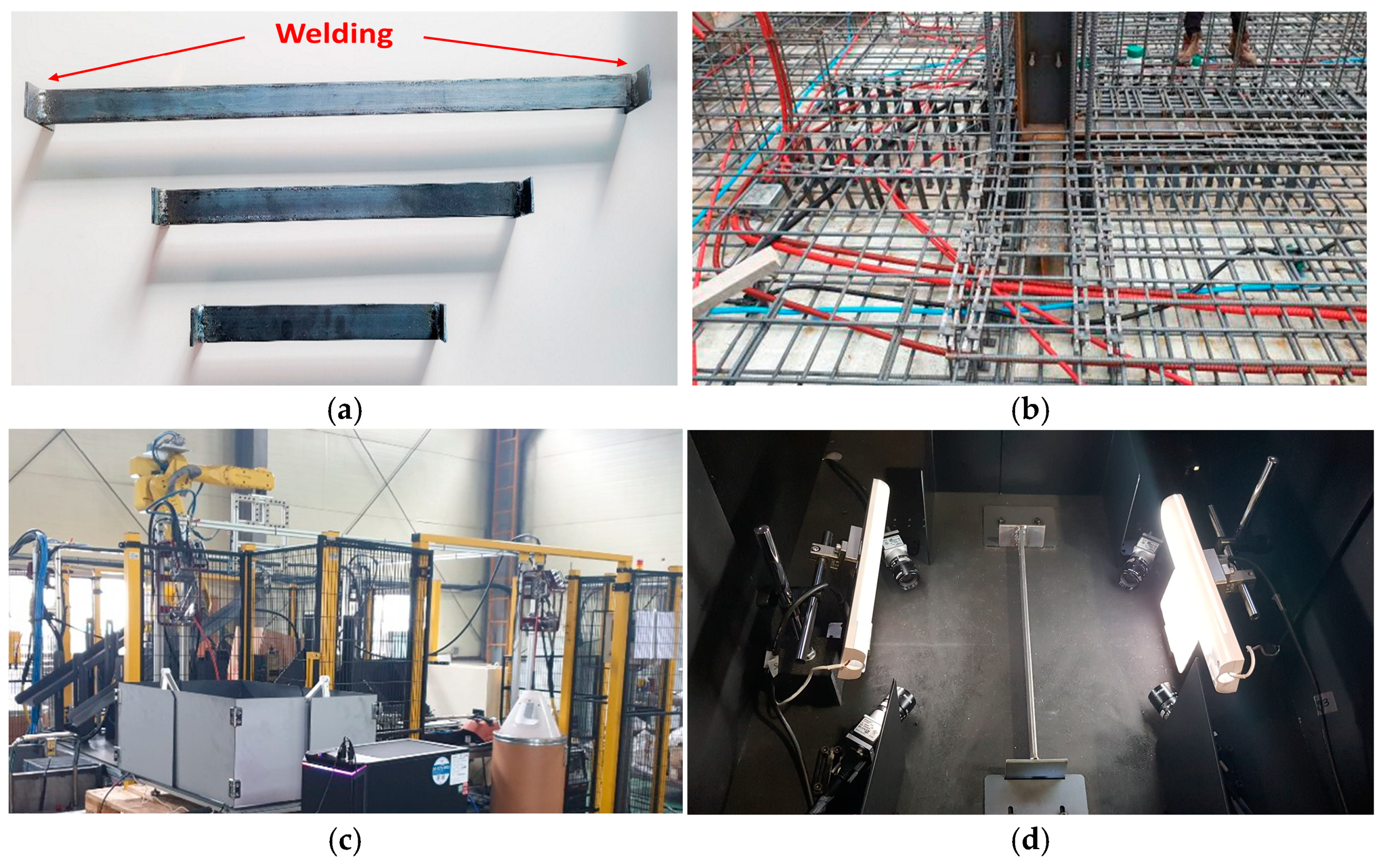
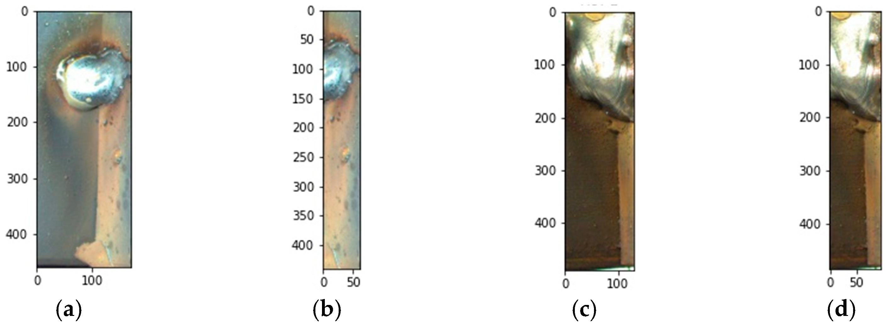
Welding is a production-based industry that is the basis for all industries, such as automobiles, construction, and shipbuilding. Among the examples in which welding is used include SRDs used in construction sites, as shown in Figure 1a,b. SRD is used to manage the shear force and shear stress of concrete structures and to improve the strength and safety of structures. In other words, welding work is very important, as SRD is directly related to safety, and inspections to check the quality of the product are essential. Therefore, when welding is performed through the machine, as shown in Figure 1c, inspection of the welding areas can be performed on the inspection table, as shown in Figure 1d. To this end, various welding quality inspection studies using sensors and image technologies have been published. At this time, the sensor inspection mainly performs the inspection using voltage, current, and gas amounts that determine the welding quality [1]. In the inspection method using sensors, various studies have been published, including a method of determining and inspecting sensor data measured in real time using a deep learning model and an inspection method of analyzing the waveforms of sensor data through deep learning [2,3,4,5,6,7,8]. In the inspection method using 2D images, methods of inspecting products for defects after dividing the welding in images taken with 2D vision cameras have been announced, and recently, methods of inspecting quality using KNN (K-nearest neighbor), K-means, improved Grabcut, etc., have been announced [9,10,11,12,13,14,15,16,17,18,19,20,21,22,23,24,25,26,27,28]. Meanwhile, sensor inspection has the advantage of high accuracy, but it also has the disadvantage in that it is impossible to check the welding location. On the other hand, 2D image inspection can determine the location of the welding bead, but if there is noise or a measurement error in the image, its accuracy decreases, and some methods have difficulty in being slow due to high calculation costs. Therefore, research is needed to solve the requirements of fast inspection time and high accuracy.
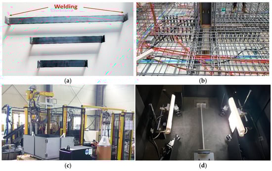
Figure 1.
SRD production and inspection: (a) SRD products; (b) construction site; (c) production machine; and (d) inspection table.
In this paper, we proposed a method that combines sensor-based inspection using average current, average voltage, and mixed gas flow rate values with 2D image inspection to address these limitations. For image inspection, we employed an image projection-based method known for its high accuracy and fast inspection speed [16]. The proposed method offers the advantage of complementing the drawbacks of sensor and image inspection methods, enabling precise inspections. Furthermore, it improves the inspection speed by making a final determination of defects without proceeding to the image inspection stage in which the sensor inspection results classify the product as bad. The remainder of this paper was organized as follows: Section 2 introduces the conventional methods for inspecting welding beads using sensor and image data. Section 3 describes the algorithm proposed in this paper, and Section 4 presents the experimental results obtained using the proposed and existing algorithms. Finally, Section 5 presents the conclusions of this study.
2. Related Works
Various inspection methods, such as sensor-based inspection and image inspection, as mentioned in the introduction, have been studied to assess the quality of welding beads. However, many small- and medium-sized enterprises still rely on visual inspection for welding quality assessments. This inspection method can suffer from reduced accuracy and slower inspection times, as the inspection results may vary depending on the inspector’s condition and expertise. Consequently, there are limitations to performing extensive inspections solely through human visual inspection.
In sensor-based inspection, data, such as real-time current, voltage, and gas flow rates, are primarily utilized for analysis. This is because welding quality is determined through various parameters during the welding process, including voltage, current, gas levels, welding time, and temperature [1]. Among the inspection methods using sensor data, several studies have been conducted, including research using real-time current and voltage data to determine the presence of the welding bead, research establishing the criteria for classifying welding bead defects using artificial neural networks (ANNs), algorithms predicting three types of defective welding conditions occurring during spot resistance welding using artificial neural network algorithms, and studies that have converted sensor data into images and train ANNs to assess welding quality [2,3,4,5]. Additionally, methods for inspecting welding quality using acoustic signals, highly correlated with current magnitude and gas supply, have been proposed [6,7,8]. Tao et al. proposed a digital twin system for weld sound detection [6]. This system utilized the SeCNN-LSTM model to recognize and classify welding quality based on the characteristics of strong acoustic signal time sequences. Gao introduced a subjective evaluation model that can detect welding process defects based on the hearing of expert welders [7]. Furthermore, Horvat proposed an algorithm for classifying welding quality by analyzing the major acoustic signals of GMAW welding [8]. However, when solely relying on sensor data for welding quality inspection, it may be possible to determine the presence of welding defects but confirming the location and shape of welding beads solely based on sensor data can be challenging, potentially leading to defects. Additionally, converting sensor data into images involves complex calculations and lengthy inspection times, and acoustic signal extraction and analysis methods can be quite intricate, making inspections not straightforward. Therefore, solely relying on sensor-based inspection for quality inspection has its limitations. Recently, research on data analysis using multi-sensor/image fusion has also been presented. Qiu et al. introduced various machine learning-based multi-sensor information fusion studies that have recently been published [9]. Of note, they have introduced wearable sensors, smart wearable devices, and key application areas, and proposed fusion methods for multi-modal and multi-location sensors. Liu et al. presented a multi-modal vision fusion model (MVFM) for comprehensive policy learning using object detection, depth estimation, and semantic segmentation [10]. However, when evaluating its practical suitability beyond the specific experimental setup, it is important to take into account its limitations related to platform specificity, data availability, and generalizability. Furthermore, Gasmi et al. explored the integration of satellite data from various sensors at different resolutions to predict topsoil clay content, finding that fused spectral band images consistently outperform spectral indices, leading to a notable 10% improvement in prediction accuracy [11]. This approach highlighted the potential of multi-sensor data fusion for soil mapping and precision agriculture, particularly in northeastern Tunisia. However, while this methodology offers valuable insights into soil attribute prediction using satellite data fusion, it has limitations related to its scope, complexity, and potential applicability to a broader range of soil properties and geographic regions.
Methods for inspecting welding bead quality using image data can be broadly categorized into image segmentation methods and machine learning (ML) methods. Image segmentation involves dividing an image into units at the pixel level to differentiate objects. Among these methods, geodesic active contour segments objects by slowly progressing along curves driven via edge components at the boundaries of the region of interest [9,10]. The morphology snake method reliably and quickly segments objects by performing morphology operations [11]. Recently, methods for welding bead segmentation using the morphological geodesic active contour (MorphGAC) algorithm have been introduced [12]. However, due to changes in the specific image’s location or its susceptibility to variations in light intensity and resolution, achieving complete image segmentation is challenging, resulting in a significant measurement error. Mlyahilu et al. proposed a segmentation method using the morphological geodesic active contour algorithm with histogram equalization to normalize the distribution of welding bead images [13]. One drawback of the morphological geodesic active contour algorithm is that it requires an appropriate adjustment of area parameters when creating bounding boxes for segmentation. However, using the same parameters for all welding bead images may lead to the inaccurate detection of welding beads. The Grabcut method is an image segmentation algorithm that extracts the foreground image rather than the background from an image. Recently, research on automatic mask generation using Grabcut and algorithms based on Mask R-CNN and Grabcut for segmenting cancer areas in images has been published [14,15]. However, the accuracy of these methods may decrease when dealing with complex backgrounds or objects that are similar to the background. Additionally, they require repetitive tasks, resulting in longer computation times. Therefore, in welding bead inspection, the similarity in color between the base material and the welding bead can lead to reduced detection performance. Recently, welding bead image inspection methods based on the image projection technique have been proposed [16]. This method uses image projection to obtain pixel values and draws an image histogram to find the x-axis value corresponding to a specific height. Then, it detects the welding bead’s area by cutting based on the x-value at that location in the region of interest (ROI). This inspection method is faster compared to other image inspections, as it examines only the ROI area, and offers high accuracy by inspecting the brightness values of all ROI regions.
In studies employing deep learning (DL), various methods, such as KNN and K-means, have been introduced. KNN is an algorithm that classifies data into clusters based on their similarity by measuring distances. Recently, research has been published on the use of S-KNN for detecting the regions of interest, background, and ambiguous areas, as well as segmenting images of crop leaf data using KNN and histograms [17,18,19]. However, KNN is computationally intensive, making it challenging to apply in real-time quality inspection. K-means is an algorithm that groups data with similar features into k clusters, widely used in image segmentation. Recent research has been published on image segmentation algorithms combining adaptive K-means and Grabcut, as well as studies on image segmentation in RGB and HSV color spaces [20,21,22,23,24,25]. Nevertheless, K-means requires users to determine the number of clusters in advance, and results can vary depending on the chosen number of clusters. Additionally, other methods have been proposed, such as a novel image segmentation approach optimized using the sine cosine algorithm (SCA), an approach analyzing welding surfaces using the faster R-CNN algorithm to determine defects, a method that segments welding areas using the entropy algorithm and evaluates defect presence through convolutional neural networks, and an approach that employs deep neural networks (DNNs) to evaluate defects after training on images captured by cameras with CCD (charge-coupled device) image sensors [26,27,28,29]. However, the accuracy of these methods may not reach levels suitable for commercial use, and further experimentation is required to account for various variables.
3. Proposed Algorithm
As previously mentioned, among the various welding quality inspections, inspections using sensor data offer speed and high accuracy, but suffer from the limitation of not being able to determine the exact welding location. On the other hand, inspections using 2D image data can identify the welding location, but they face several challenges, such as low accuracy when the image contains noise and measurement errors, as well as high computational costs. In this paper, to address these issues, we proposed an inspection method that combines sensor data inspection with 2D image data inspection. For 2D image data inspection, we utilized the image projection method proposed by Lee et al. [16]. This proposed method complements the strengths and weaknesses of sensor and image data inspections, effectively resolving the existing accuracy issues. Furthermore, if a defect is determined in the sensor data inspection, the inspection skips the image data inspection and directly concludes it as bad, reducing unnecessary computation and time to improve the inspection speed. The procedure of the proposed method is shown in Figure 2.
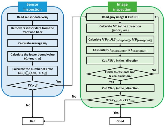
Figure 2.
Procedures of the proposed algorithm.
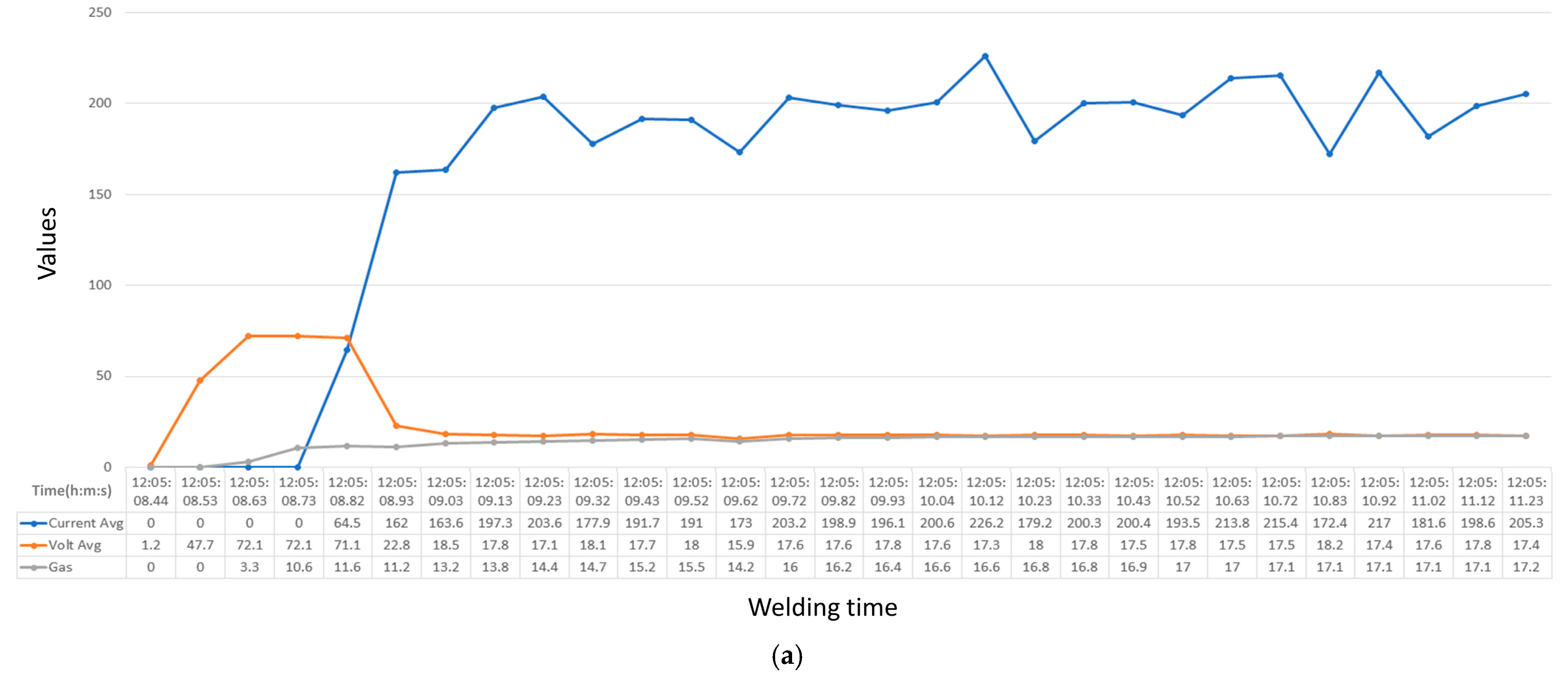
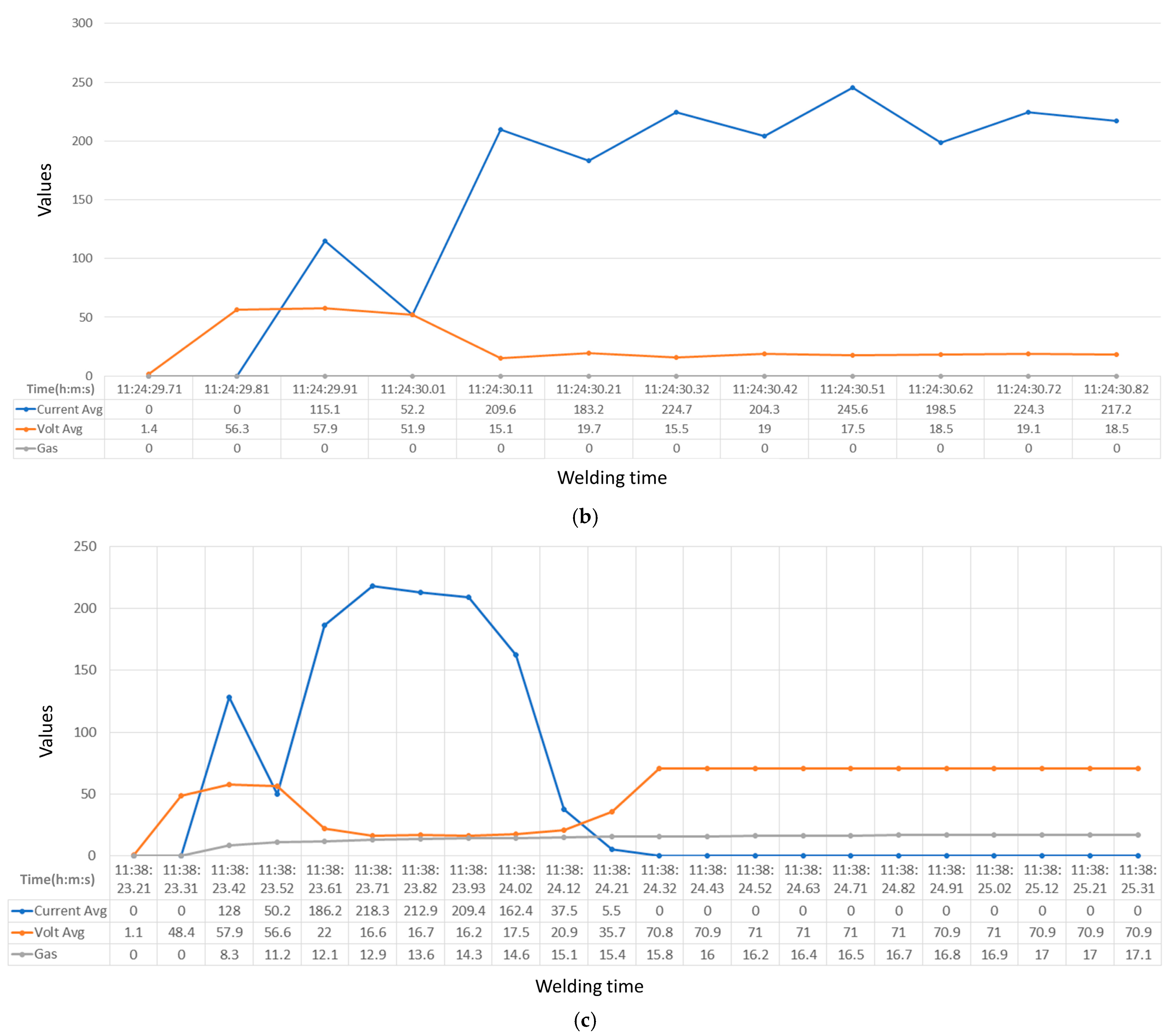
In sensor data inspection, welding bead defects are assessed using average current, average voltage, and mixed gas flow data. The mixed gas used is a combination of argon and carbon dioxide gas () to prevent contamination. Therefore, we displayed the three values generated during one welding operation on a single graph, as shown in Figure 3. When plotting some of the measured sensor data values for a single product welding, as shown in Figure 3a, the blue line represents the average current value, the orange line represents the average voltage value, and the gray line represents the mixed gas value.
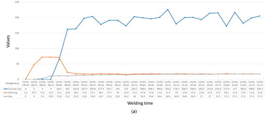
Figure 3.
Sensor results: (a) good; (b) bad—gas; (c) bad—current avg.
The current average and voltage average represent the average values obtained from the current and voltage, respectively. The x-axis represents the welding time, and the y-axis represents the values. In Figure 3a, the work took place from 12:05:08.44 to 12:05:11.23. At 12:05:08.44, the current average value was 0, the voltage average was 1.2, and the gas value was 0. Figure 3a represents the normal data. However, Figure 3b depicts the gas defective data, with all values being 0 due to an issue with gas, while Figure 3c displays the current defective data, where the current becomes problematic and results in a value of zero from the middle. In other words, when defects occur in the sensor data, the values tend to either be zero or very small.
In each sensor dataset, the approximated three values at the beginning and end were unstable, so these values were first removed. Then, the average value () was calculated for each of the three sensor datasets, where represents the average current, average voltage, and mixed gas flow, respectively. The lower bounds () were calculated for the previously calculated average values () using a threshold value (), and the formula is as follows:
The error counts () were calculated for each of the three sensor datasets, as shown in Equation (2), for sensor data () that were smaller than the sensor’s lower bounds (), which were calculated using Equation (1). Next, the error counts () calculated in Equation (2) were then evaluated against a threshold value (), as described in Equation (3). If , it was considered as a good product, whereas if , it was considered as a bad product.
In the sensor data inspection, if any one of the three sensors was determined as bad, the product was ultimately classified as bad, and the inspection was proceeded to the next product. On the other hand, if all three sensors were deemed as good, the image data inspection was performed.
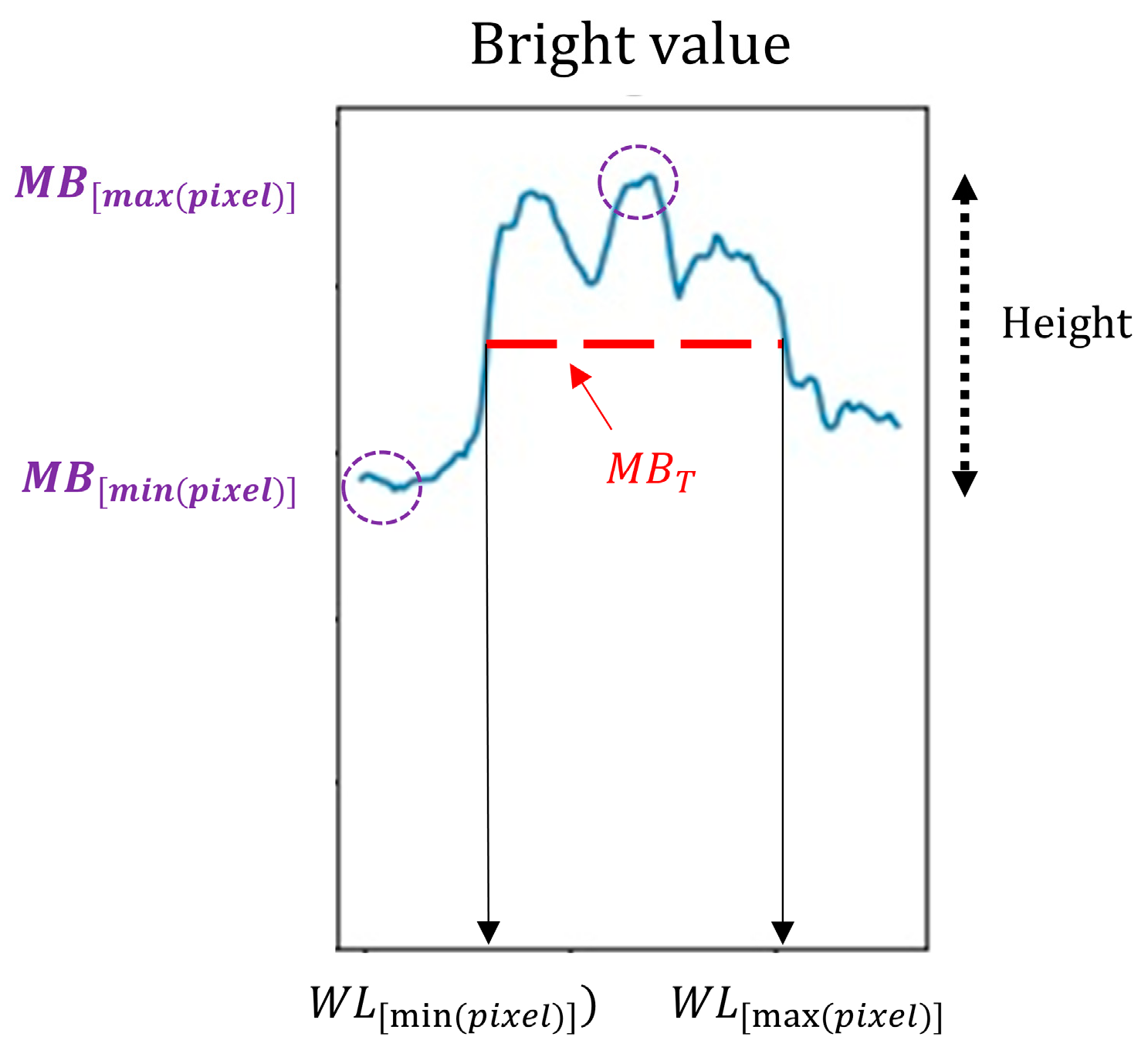
In the image data inspection, the welding area was extracted and its major dimensions were measured to detect welding defects using the image inspection method based on the image projection algorithm [16]. For color image data, each pixel value () was represented as , where corresponds to color channels (red: zero, green: one, and blue: two). We calculated the mean brightness () in the vertical direction in the ROI of the image using Equation (4):
where represents the starting position of the y-axis in the image, and represents the ending position of the y-axis. Regarding the mean brightness in the vertical direction, as shown in Figure 4, we made an image histogram and then calculated the maximum value () and the lowest value () on the y-axis. Next, we calculated the position corresponding to 50% of the height, as described in Equation (5).
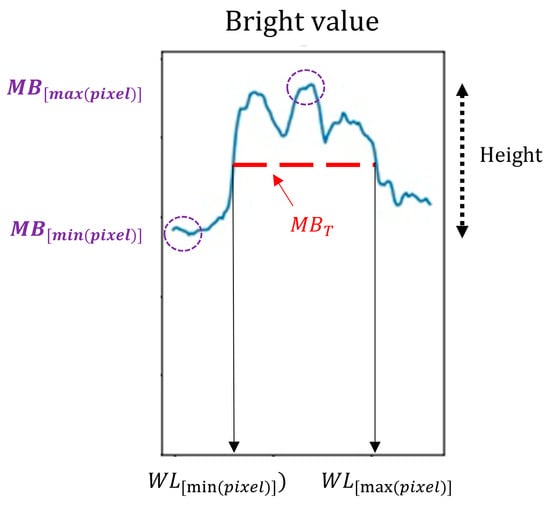
Figure 4.
The process of calculating and .
Using the calculated value obtained above, we found the minimum () and maximum () values on the x-axis, and then cut the ROI based on these values. and represent the x-axis positions where it has been presumed that the welding bead exists within the ROI. The same procedure was followed for the horizontal direction, and in this case, the mean brightness () in the horizontal direction was calculated following Equation (6):
where represents the starting position of the x-axis in the image, and represents the ending position of the x-axis. Using the values calculated in both the vertical and horizontal directions, the dimensions of the welding bead were measured in the extracted region of the welding bead. Then, the threshold values and were used in Equations (7) and (8) below. If the calculated values exceed these threshold values, the product was considered good; otherwise, it was classified as bad.
4. Experimental Results
In this section, experiments were conducted to determine the quality of welding beads using the proposed method, which utilized sensor data, such as average current, average voltage, and mixed gas data generated during welding, as well as image data. Additionally, comparative experiments with existing algorithms were conducted to evaluate the performance of the proposed approach.
4.1. Experiment Setups
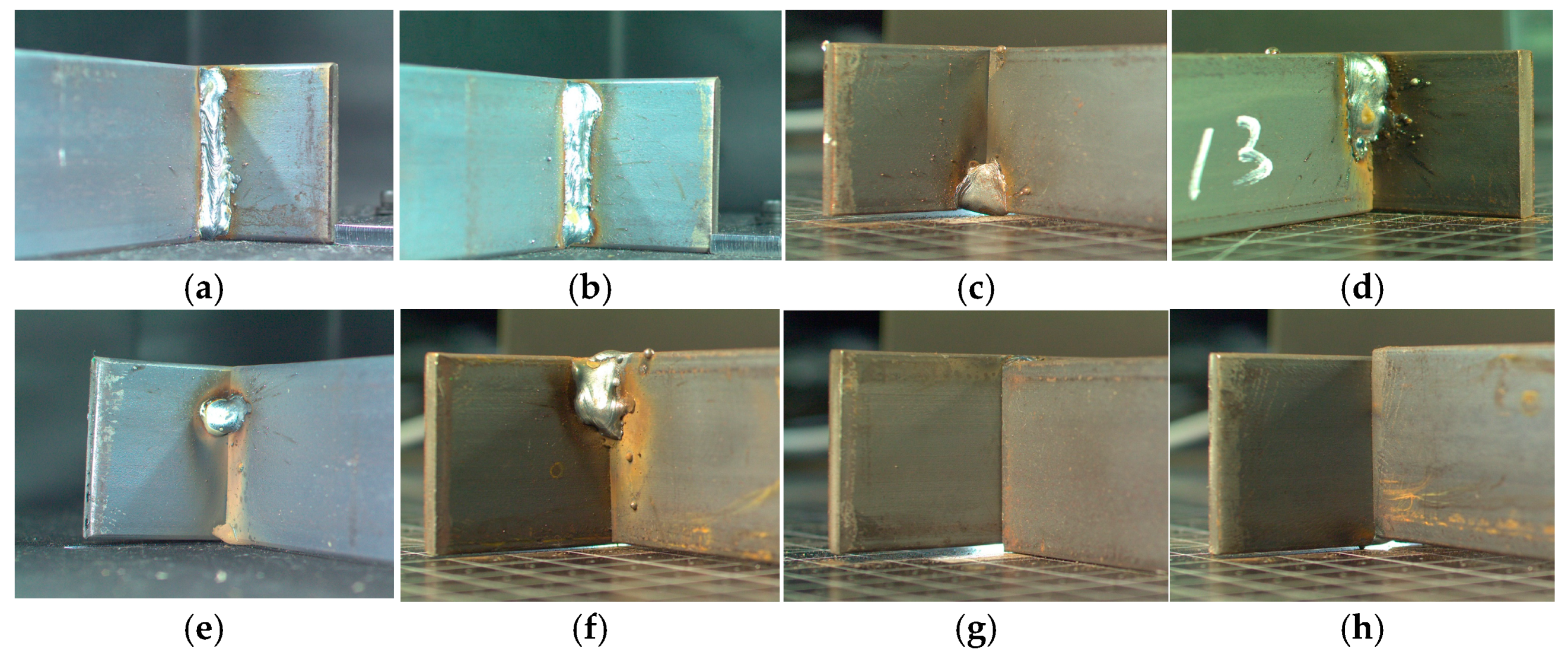
In this experiment, sensor data and image data generated during the production of SRDs were analyzed. A total of 412 SRD welding beads were analyzed, consisting of 400 good samples and 12 bad samples. Regarding the sensor data, good samples exhibited outputs, as shown in Figure 3a, while in cases of defects, current, voltage, or mixed gas values were either entirely or partially unused, resulting in data values of zero or small values, as seen in Figure 3b,c. In the image data, good samples were represented as shown in Figure 5a,b, whereas bad samples exhibited characteristics where only a portion of the welding bead is present, as shown in Figure 5c–f or, in extreme cases, where no welding bead is present at all, as shown in Figure 5g,h. The input image dimensions were 256 by 256. The experiments were conducted under conditions of approximately 700 Lux illumination and an average brightness of about 200 for the welding bead. For setting the threshold values in the sensor data, experiments were conducted with variations in the and values, and the results showed that the highest accuracy was achieved when and were both set to 0.5 and 5, respectively, as shown in Table 1. Therefore, these values were chosen as the threshold values for analysis.

Figure 5.
The SRD welding bead products: (a) good-1; (b) good-2; (c) bad-1; (d) bad-2; (e) bad-3; (f) bad-4; (g) bad-5; (h) bad-6.

Table 1.
Sensor inspection results according to and .
The PC specifications were as follows: Windows 10 Pro, i9 with NVIDIA GeForce RTX 3080 (NVIDIA, Santa Clara, CA, USA) with GDDR6X 10GB, 3.7 GHz per processor, and Python 3.8.
4.2. Experiment Results
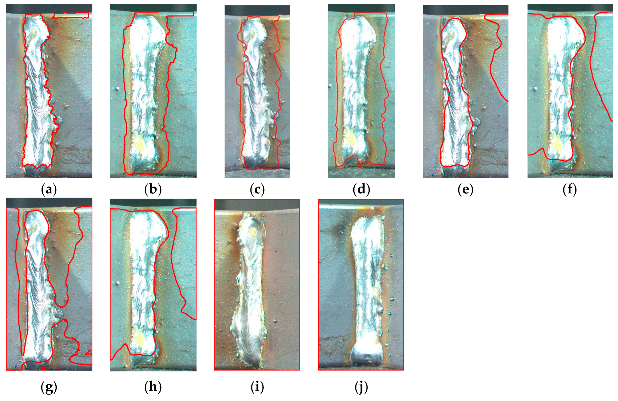
First, experiments were conducted separately for the sensor inspection, image inspection, and the combined inspection method proposed in this study, and the results are shown in Table 2. For the good samples, all three inspection methods accurately classified them as good. However, in the sensor inspection, one bad sample was not classified, and in the image inspection, two bad samples were not classified. In contrast, the combined inspection method successfully classified all the bad samples. The results of the image inspection performed in this study are shown in Figure 6, Figure 7 and Figure 8. Figure 6 shows the results of testing the good samples, where Figure 6a,c represent the ROI of the welding bead, Figure 6b shows the result of detecting the welding bead from Figure 6a, and Figure 6d shows the result of detecting the welding bead from Figure 6c. Figure 7 displays the results of testing the bad samples, where Figure 7a,c represent the detected width of the welding bead, and Figure 7b,d represent the detected height. As observed in the results of the image inspection, some measurement errors occurred, but it was possible to detect the significant width and height of the welding bead. On the other hand, Figure 8 shows two bad samples that were not classified during the image inspection experiments. In other words, these are incorrectly inspected image results. Figure 8a,c represent the results of detecting the width of the welding bead, while Figure 8b,d represent the results of detecting its height. As evident from the experimental results in Figure 8, it was possible to detect the width of the welding bead, but its height remained undetected. Consequently, in image inspection, what was actually ‘bad’ was misclassified as ‘good’ in the inspection results. This was attributed to the small size of the welding beads and the high brightness values of the base material, resulting in a small difference between and in the image histogram, as shown in Figure 4.
Table 2.
Confusion matrix of the proposed algorithms.
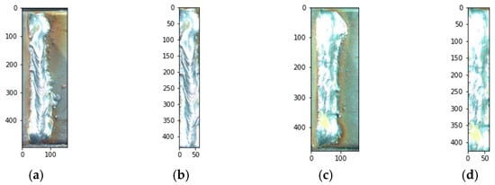
Figure 6.
The ROI and proposed inspection results of good SRD welding bead products. (a) The ROI of good-1. (b) The segmentation result of good-2. (c) The ROI of good-2. (d) The segmentation result of good-2.
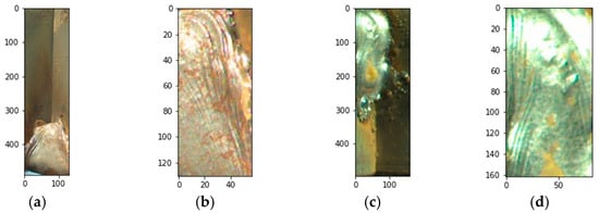
Figure 7.
The proposed inspection results of bad SRD welding bead products. (a) Vertical direction inspection of bad-1. (b) Horizontal direction inspection of bad-1. (c) Vertical direction inspection of bad-2. (d) Horizontal direction inspection of bad-2.
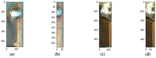
Figure 8.
Experimental results of the proposed method for misclassified bad products. (a) Vertical direction inspection of bad-3. (b) Horizontal direction inspection of bad-3. (c) Vertical direction inspection of bad-4. (d) Horizontal direction inspection of bad-4.
Based on the confusion matrix, we calculated several evaluation metrics, such as accuracy, precision, recall, and F1 score, using the following formulas:
We calculated the performance metrics outlined in Table 2 using the four evaluation metrics mentioned above, and the results are shown in Table 3. In sensor inspection, image inspection, and combined inspection, all performance metric values exceeded 99%, with computation times of 2 s, 27 s, and 26 s, respectively. This indicates that each inspection method individually achieved a sufficiently high performance. However, the combined method of the two inspection approaches allowed for the accurate classification of all experimental data. In addition, when conducting sensor inspection alone, it only took 2 s, but when combining image inspection into the combined inspection, it can be concluded that there was only a slight improvement in performance, while significantly sacrificing in terms of its speed. However, it is crucial to verify whether the welding bead is properly placed (position) and whether the width and size of the welding bead are consistent (shape), as it is related to its safety. When using sensor inspection alone, it was not possible to confirm the location and shape of the welding. Therefore, when conducting sensor and image inspections together, it was possible to perform accurate inspections. Furthermore, in order to increase the speed of image inspection, we reduced the resolution. However, due to its reduced accuracy, we analyzed it at a size of 256 × 256. Therefore, the proposed method was confirmed to complement the drawbacks of sensor inspection and image inspection, resulting in its excellent performance and fast computational speed.
Table 3.
Classification evaluation metrics and computation times of the proposed algorithms.
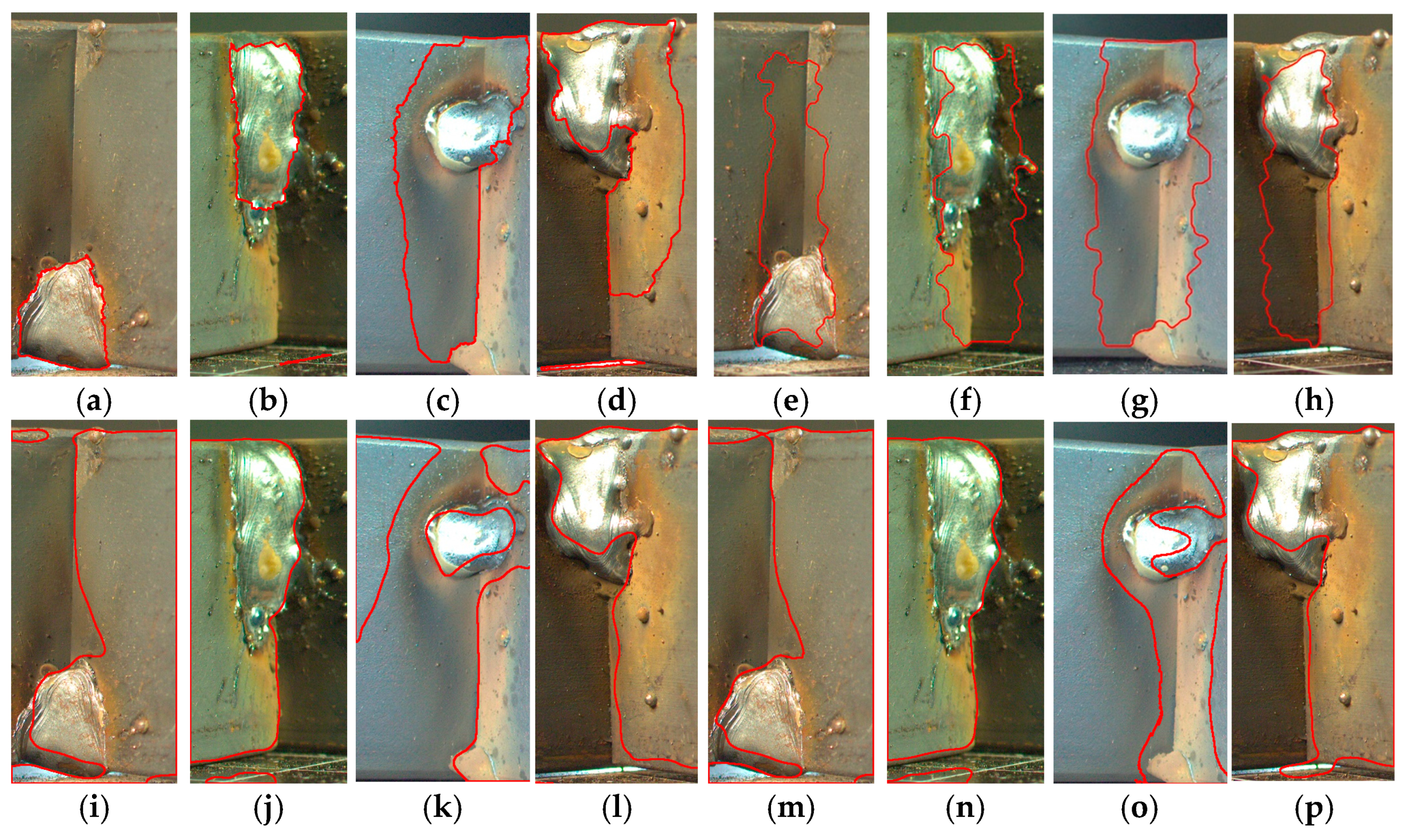
To evaluate the performance of the proposed method, comparative experiments were conducted using existing methods. Among the existing methods, we conducted experiments with improved Grabcut [20], morphological geodesic active contour with Canny [13], KNN, K-means with HSV [22], and clustering with the SCA [26]. Initially, these experiments were performed on two good samples for each method, and the results are shown in Figure 9. Each method highlights detected areas in red as shown in Figure 9. From the experimental results, it was observed that all methods detected more areas than the actual welding bead regions. In particular, as shown in Figure 9g–j, K-means with HSV and clustering with the SCA failed to detect welding beads to a large extent. Next, we conducted experiments using existing methods on the bad images in Figure 5c–f, and the results are shown in Figure 10. As observed in Figure 10, similar to Figure 9, detected areas for each method are highlighted in red. As seen in Figure 10a,b, improved Grabcut performed the best in detecting the welding beads, while the other methods detected more areas than the actual welding bead region. Additionally, as shown in Figure 8, the two images that the proposed method failed to detect were also not detected using the existing methods. In particular, clustering failed to even detect the shape of the welding beads. Based on the results of the welding bead detection experiments using existing methods, we conducted classification tests for the good and bad products, and the results are presented in Table 4 and Table 5. Table 4 shows the confusion matrix. As observed in Table 4, K-means with HSV had the highest number of misclassifications, misclassifying good products as bad in 109 cases. Furthermore, morphological geodesic active contour with Canny, KNN, and clustering with the SCA failed to detect any bad products. Table 5 shows the performance metrics that were calculated based on the results of Table 4. Among the existing methods, improved Grabcut exhibited the highest performance metrics, followed by morphological geodesic active contour with Canny and clustering with the SCA, and then, in order, KNN and K-means with HSV. While K-means with HSV had the highest precision of 97.73, it misclassified approximately 1/4 of the good products, resulting in the lowest accuracy, recall, and F1 score values. Among the existing methods, improved Grabcut had the highest performance, but the proposed method was able to accurately classify all welding beads. Furthermore, improved Grabcut had a computation time of 690.75 s, which was considerably high. In contrast, our proposed method had the shortest computation time of 25.736 s.
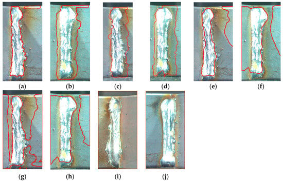
Figure 9.
Existing algorithm results of good SRD welding bead products. (a) Improved Grabcut results of good-1. (b) Improved Grabcut results of good-2. (c) MorphGAC with Canny results of good-1. (d) MorphGAC with Canny results of good-2. (e) KNN results of good-1. (f) KNN results of good-2. (g) K-means with HSV results of good-1. (h) K-means with HSV results of good-2. (i) Clustering with the SCA results of good-1. (j) Clustering with the SCA results of good-2.
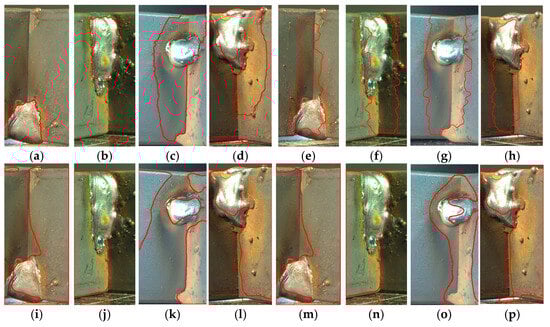
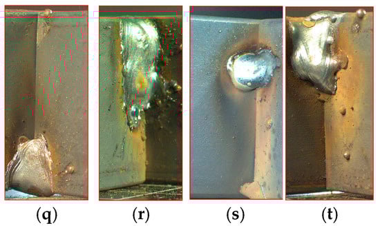
Figure 10.
Existing algorithm results of bad SRD welding bead products. (a) Improved Grabcut results of bad-1. (b) Improved Grabcut results of bad-2. (c) Improved Grabcut results of bad-3. (d) Improved Grabcut results of bad-4. (e) MorphGAC with Canny results of bad-1. (f) MorphGAC with Canny results of bad-2. (g) MorphGAC with Canny results of bad-3. (h) MorphGAC with Canny results of bad-4. (i) KNN results of bad-1. (j) KNN results of bad-2. (k) KNN results of bad-3. (l) KNN results of bad-4. (m) K-means with HSV results of bad-1. (n) K-means with HSV results of bad-2. (o) K-means with HSV results of bad-3. (p) K-means with HSV results of bad-4. (q) Clustering with the SCA results of bad-1. (r) Clustering with the SCA results of bad-2. (s) Clustering with the SCA results of bad-3. (t) Clustering with the SCA results of bad-4.
Table 4.
A confusion matrix of the proposed and comparison algorithms.
Table 5.
Classification evaluation metrics and computation times of the proposed and comparison algorithms.
5. Conclusions
In welding bead inspection, sensor-based inspection offers high accuracy in determining the presence of welding but cannot pinpoint the exact location of the welding bead. On the other hand, 2D image inspection can identify the location of the welding bead but may have a lower level of inspection accuracy compared to sensor-based inspection and involves significant computational costs. To address these limitations, this paper proposed a welding bead defect inspection method that combines sensor-based inspection and 2D image inspection. In sensor-based inspection, a method was proposed to determine defect presence based on patterns in average current, average voltage, and mixed gas flow. In image inspection, the image inspection method based on image projection was utilized [16]. The proposed inspection method, if determined as bad in sensor-based inspection, skips the image inspection step and ultimately classifies it as bad, reducing unnecessary computation and inspection times. Experimental results showed that accuracy in sensor-based and image inspections was 99.8% and 99.59%, respectively, while the combined method achieved 100% accuracy. This demonstrates that the proposed method enhances inspection accuracy by overcoming the limitations of each individual method. Furthermore, comparative experiments evaluating the proposed method’s performance showed that among the existing methods, improved Grabcut achieved the highest accuracy at 98.98%. However, when compared to the proposed method, it had the highest performance and computational speed.
In future work, we plan to conduct research aimed at implementing an automation system that can be applied in real industrial settings using the proposed method. Additionally, we intend to experiment with different welding products to generalize the proposed method.
Author Contributions
Conceptualization, J.L. and J.K.; methodology, J.L. and J.K.; software, J.L. and J.K.; validation, J.L., H.C. and J.K.; formal analysis, J.L. and J.K.; investigation, J.L. and J.K.; resources, J.L. and J.K.; data curation, J.L. and J.K.; writing—original draft preparation, J.L.; writing—review and editing, H.C. and J.K.; visualization, J.K.; supervision, J.K.; project administration, J.K.; funding acquisition, J.K. All authors have read and agreed to the published version of the manuscript.
Funding
This research was funded by the Small and Medium Business Technology Innovation Development Project from TIPA, grant number 00220304 and 00278083, the National Research Foundation of Korea, grant number CD202112500001, and Link 3.0 of PKNU, grant number 202310810001.
Institutional Review Board Statement
Not applicable.
Informed Consent Statement
Not applicable.
Data Availability Statement
Not applicable.
Conflicts of Interest
The authors declare no conflict of interest.
References
- Kurt, H.I.; Oduncuoglu, M.; Yilmaz, N.F.; Ergul, E.; Asmatulu, R. A comparative study on the effect of welding parameters of austenitic stainless steels using artificial neural network and Taguchi approaches with ANOVA analysis. Metals 2018, 8, 326. [Google Scholar] [CrossRef]
- Kim, M.S.; Shin, S.M.; Kim, D.H.; Rhee, S.H. A study on the algorithm for determining back bead generation in GMA welding using deep learning. J. Weld. Join. 2018, 36, 74–81. [Google Scholar] [CrossRef]
- Kim, J.H.; Ko, M.H.; Ku, N.K. A Study on Resistance Spot Welding Failure Detection Using Deep Learning Technology. J. Comp. Des. Eng. 2019, 24, 161–168. [Google Scholar]
- Hwang, I.S.; Yoon, H.S.; Kim, Y.M.; Kim, D.C.; Kang, M.J. Prediction of irregular condition of resistance spot welding process using artificial neural metwork. In Proceedings of the 2017 Fall Conference of Society for The Korean Welding & Joining Society, Daegu, Republic of Korea, 30 November 2017. [Google Scholar]
- Kang, J.H.; Ku, N.K. Verification of Resistance Welding Quality Based on Deep Learning. J. Soc. Nav. Archit. Korea 2019, 56, 473–479. [Google Scholar] [CrossRef]
- Ji, T.; Mohamad Nor, N. Deep Learning-Empowered Digital Twin Using Acoustic Signal for Welding Quality Inspection. Sensors 2023, 23, 2643. [Google Scholar] [CrossRef]
- Gao, Y.; Zhao, J.; Wang, Q.; Xiao, J.; Zhang, H. Weld bead penetration identification based on human-welder subjective assessment on welding arc sound. Measurement 2020, 154, 107475. [Google Scholar] [CrossRef]
- Horvat, J.; Prezelj, J.; Polajnar, I.; Cudina, M. Monitoring Gas Metal Arc Welding Process by Using Audible Sound Signal. J. Mech. Eng. 2011, 57, 267–278. [Google Scholar] [CrossRef]
- Wang, Z.; Liu, Y. Active contour model by combining edge and region information discrete dynamic systems. Adv. Mech. Eng. 2017, 9, 1–10. [Google Scholar] [CrossRef]
- Ma, J.; Wang, D.; Wang, X.P.; Yang, X. A Fast Algorithm for Geodesic Active Contours with Applications to Medical Image Segmentation. arXiv 2020, arXiv:2007.00525. [Google Scholar]
- Yin, X.X.; Jian, Y.; Zhang, Y.; Zhang, Y.; Wu, J.; Lu, H.; Su, M.Y. Automatic breast tissue segmentation in MRIs with morphology snake and deep denoiser training via extended Stein’s unbiased risk estimator. Health Inf. Sci. Syst. 2021, 9, 16. [Google Scholar] [CrossRef]
- Mlyahilu, J.; Kim, Y.B.; Lee, J.E.; Kim, J.N. An Algorithm of Welding Bead Detection and Evaluation Using and Multiple Filters Geodesic Active Contour. JKICSP 2021, 22, 141–148. [Google Scholar]
- Mlyahilu, J.N.; Mlyahilu, J.N.; Lee, J.E.; Kim, Y.B.; Kim, J.N. Morphological geodesic active contour algorithm for the segmentation of the histogram-equalized welding bead image edges. IET Image Process. 2022, 16, 2680–2696. [Google Scholar] [CrossRef]
- Wu, H.; Liu, Y.; Xu, X.; Gao, Y. Object Detection Based on the GrabCut Method for Automatic Mask Generation. Micromachines 2022, 13, 2095. [Google Scholar] [CrossRef]
- Saranya, M.P.; Praveena, V.; Dhanalakshmi, M.B.; Karpagavadivu, M.K.; Chinnasamy, P. Diagnosis of gastric cancer using mask R–CNN and Grabcut segmentation method. J. Posit. Sch. Psychol. 2022, 6, 203–206. [Google Scholar]
- Lee, J.; Choi, H.; Kim, J. Inspection Algorithm of Welding Bead Based on Image Projection. Electronics 2023, 12, 2523. [Google Scholar] [CrossRef]
- Wazarkar, S.; Keshavamurthy, B.N.; Hussain, A. Region-based segmentation of social images using soft KNN algorithm. Procedia Comput. Sci. 2018, 125, 93–98. [Google Scholar] [CrossRef]
- Rangel, B.M.S.; Fernández, M.A.A.; Murillo, J.C.; Ortega, J.C.P.; Arreguín, J.M.R. KNN-based image segmentation for grape-vine potassium deficiency diagnosis. In Proceedings of the 2016 IEEE International Conference on Electronics, Communica-tions and Computers (CONIELECOMP), Cholula, Mexico, 24–26 February 2016; pp. 48–53. [Google Scholar]
- Hossain, E.; Hossain, M.F.; Rahaman, M.A. A color and texture based approach for the detection and classification of plant leaf disease using KNN classifier. In Proceedings of the 2019 International Conference on Electrical, Computer and Communication Engineering (ECCE), Cox’sBazar, Bangladesh, 7–9 February 2019; pp. 1–6. [Google Scholar]
- Prabu, S. Object Segmentation Based on the Integration of Adaptive K-means and GrabCut Algorithm. In Proceedings of the IEEE 2022 International Conference on Wireless Communications Signal Processing and Networking (WiSPNET), Chennai, India, 24–26 March 2022; pp. 213–216. [Google Scholar]
- Nasor, M.; Obaid, W. Segmentation of osteosarcoma in MRI images by K-means clustering, Chan-Vese segmentation, and iterative Gaussian filtering. IET Image Process. 2021, 15, 1310–1318. [Google Scholar] [CrossRef]
- Hassan, M.R.; Ema, R.R.; Islam, T. Color image segmentation using automated K-means clustering with RGB and HSV color spaces. J. Comput. Sci. Technol. 2017, 17, 26–33. [Google Scholar]
- Qiao, D.; Zhang, X.; Ren, Y.; Liang, J. Comparison of the Rock Core Image Segmentation Algorithm. In Proceedings of the 2022 IEEE 7th International Conference on Image, Vision and Computing (ICIVC), Xi’an, China, 26–28 July 2022; pp. 335–339. [Google Scholar]
- Debelee, T.G.; Schwenker, F.; Rahimeto, S.; Yohannes, D. Evaluation of modified adaptive k-means segmentation algorithm. Comput. Vis. Media. 2019, 5, 347–361. [Google Scholar] [CrossRef]
- Zheng, X.; Lei, Q.; Yao, R.; Gong, Y.; Yin, Q. Image segmentation based on adaptive K-means algorithm. EURASIP J. Image Video Process. 2018, 1, 68. [Google Scholar] [CrossRef]
- Khrissi, L.; El Akkad, N.; Satori, H.; Satori, K. Clustering method and sine cosine algorithm for image segmentation. Evol. Intell. 2022, 15, 669–682. [Google Scholar] [CrossRef]
- Baek, J.W.; Kong, S.G. Faster R-CNN Classifier Structure Design for Detecting Weld Surface Defects. In Proceedings of the KIIT Conference, Washington, DC, USA, 27–28 July 2018; pp. 149–152. [Google Scholar]
- Haffner, O.; Kučera, E.; Drahoš, P.; Cigánek, J. Using Entropy for Welds Segmentation and Evaluation. Entropy 2019, 21, 1168. [Google Scholar] [CrossRef]
- Kim, T.W.; Han, C.M.; Choi, H.W. Welding Quality Inspection using Deep Learning. In Proceedings of the KSMPE Conference, Tongyeong, Republic of Korea, 25–26 June 2020; p. 18. [Google Scholar]


Disclaimer/Publisher’s Note: The statements, opinions and data contained in all publications are solely those of the individual author(s) and contributor(s) and not of MDPI and/or the editor(s). MDPI and/or the editor(s) disclaim responsibility for any injury to people or property resulting from any ideas, methods, instructions or products referred to in the content. |
© 2023 by the authors. Licensee MDPI, Basel, Switzerland. This article is an open access article distributed under the terms and conditions of the Creative Commons Attribution (CC BY) license (https://creativecommons.org/licenses/by/4.0/).