Article

Cardiac Electrophysiology Meshfree Modeling through the Mixed Collocation Method

by
Konstantinos A. Mountris
1,2,† and
Esther Pueyo
1,2,*,†
1
Aragón Institute for Engineering Research, University of Zaragoza, IIS Aragón, 50018 Zaragoza, Spain
2
CIBER in Bioengineering, Biomaterials & Nanomedicine (CIBER-BBN), 50018 Zaragoza, Spain
*
Author to whom correspondence should be addressed.
These authors contributed equally to this work.
Appl. Sci. 2023, 13(20), 11460; https://doi.org/10.3390/app132011460
Submission received: 8 September 2023 / Revised: 12 October 2023 / Accepted: 16 October 2023 / Published: 19 October 2023
(This article belongs to the Section Biomedical Engineering)

Abstract

:
We present the meshfree mixed collocation method (MCM) for cardiac electrophysiology simulation. Capitalizing on the meshfree property of MCM, we introduce an immersed grid approach for automated generation of meshfree node grids from medical image data. This approach allows us to avoid the time-consuming mesh generation and processing that mesh-based methods like the finite element method (FEM) require. We employ the MCM to solve the cardiac monodomain model considering electrical propagation in 2D tissue sheets, 3D tissue slabs, and a realistic biventricular anatomy. We demonstrate that the solutions obtained by the MCM are in good agreement with the FEM, particularly when immersed grid is used. These findings confirm the suitability of the MCM for cardiac electrophysiology simulation and make the MCM a promising alternative to the FEM for cardiac electrical investigations.

1. Introduction

In the last decades, computational modeling and simulation has taken a growing role as a method to deepen the understanding of cardiac function in health and disease [1,2]. Novel in silico models of increasing complexity are continuously being developed to simulate the electrophysiology [3] and mechanics of the heart [4] from the cell [5] to the whole-organ level [6]. At the tissue and organ levels, electrophysiology is simulated by using the well-known bidomain [7] and monodomain [8] models. The latter is a simplified version of the former under the assumption of equal anisotropy ratios for the intracellular and extracellular spaces. The monodomain model is more computationally efficient than its bidomain counterpart and is able to produce accurate transmembrane potential values in the absence of extracellularly applied currents [9]. Commonly, state-of-the-art simulators [10,11] employ the finite element method (FEM) to solve either the bidomain or the monodomain model for the simulation of cardiac electrophysiology. FEM is a mature and robust numerical method, but its requirement for a good-quality mesh may pose challenges to generate realistic heart models with reasonable computational cost [12].
Alternative meshfree methods can alleviate the mesh requirement and have been proposed for both cardiac electrophysiological [13,14,15] and mechanical [12,16] simulations, as well as brain biomechanics [17]. Among the different proposed meshfree solutions, models based on the element-free Galerkin (EFG) method offer high convergence rate and high resolution of localized steep gradients [18]. Nevertheless, special treatment for the imposition of essential boundary conditions is required since the approximation functions do not possess the Kronecker delta property. Recently, cell-based maximum entropy (CME) approximants were used in the EFG method to alleviate this limitation [19].
CME possesses the weak Kronecker delta property where approximation functions of internal nodes vanish on the boundaries. Therefore, essential boundary conditions can be imposed directly, as in the FEM. However, the CME approximants give rise to complex integrals requiring a large number of quadrature points for accurate integration that may lead to increased computational cost. Similarly, the computational cost of methods based on smoothed particle hydrodynamics (SPH) may be significantly higher than that of mesh-based methods. Furthermore, the standard SPH formulation may imply inaccurate computation of gradients of constant and linear fields (first-order incomplete approximation) [20]. To overcome these problems, the total Lagrangian formulation of SPH [21] and gradient normalization [20] were applied in [12,13] to accurately simulate the propagation of the electrical impulse in the heart and cope with large deformations in the context of cardiac mechanics.
In the present study, we propose the mixed collocation method (MCM) as an alternative to mesh-based and previously mentioned meshfree methods for cardiac electrophysiology simulation. Our main motivation is the purely meshfree property of MCM that allows us to completely alleviate the time-consuming mesh-generation process of mesh-based methods like the FEM. The MCM is based on the meshfree local Petrov–Galerkin (MLPG) method [22,23]. MLPG implies quadrature over locally-defined domains, providing the flexibility to select the trial and test functions from different spaces. In the mixed collocation variant of the MLPG method, the Dirac function is used as test function, and both the field function and its gradient are interpolated by the trial function. As a result, the computational cost is decreased since the local integration is reduced to nodal summation. Moreover, while collocation methods suffer from inaccurate imposition of Neumann boundary conditions [24], the accuracy is ameliorated in the MCM due to the interpolation of the field function’s gradient. In the seminal work on the MCM [25], the moving least squares (MLS) approximation [26] was used as the trial function. Recently, the radial point interpolation (RPI) [27] was proposed as an alternative to MLS in the MCM [28]. It was demonstrated that accuracy is improved when RPI trial functions replace MLS. This was mainly attributed to the delta Kronecker property of RPI that allows the direct imposition of essential boundary conditions in contrast to MLS.
Here, we investigate the application of the MCM with interpolating trial functions for the solution of the monodomain equation in a series of cardiac electrophysiology simulations in 2D and 3D domains. We evaluate RPI as well as moving kriging interpolation (MKI) [29] and we compare the obtained solutions with the state-of-the-art FEM solution. Moreover, we propose an immersed grid generation approach to automatically obtain nodal distributions from segmentated data of medical images. The structure of the paper is the following. In Section 2, we derive the form of the cardiac monodomain equation using the MCM method and describe the mathematical formulation of RPI and MKI interpolations. In Section 3, we evaluate the solution of the monodomain model with the MCM method in several 2D and 3D problems and we report on the accuracy and efficiency of the method in comparison to FEM. Finally, in Section 4, we discuss some concluding remarks.

2. Materials and Methods

2.1. Mixed Collocation Form of the Monodomain Equation

The propagation of an electrical impulse in the heart is modeled through the monodomain model by the reaction–diffusion equation:
V t = · ( D V ) 1 C I i o n ( s , V , t ) in Ω s t = f ( s , V , t ) in Ω n · ( D V ) = 0 on Ω
where V / t is the time derivative of the transmembrane potential V = V ( t ) and s is the vector of cellular gating variables and ionic concentrations. The function f ( s , V , t ) describes the nonlinear cellular dynamics. I i o n ( s , V , t ) denotes the ionic current per cell membrane area and C the capacitance of the cell membrane per unit area. Ω represents the domain of interest and Ω its boundary, while n is the outward unit vector normal to Ω . D is the diffusion tensor given by
D = d 0 ( 1 ρ ) l l + ρ I
where d 0 denotes the diffusion coefficient along the cardiac fibers, ρ 1 is the transverse-to-longitudinal conductivity ratio, l denotes the cardiac fiber direction vector, I is the identity matrix, and ⊗ is the tensor product operation.
The nonlinear cellular dynamics involved in the computation of I i o n make the solution of the coupled model in Equation (1) cumbersome. For large-scale tissue simulations, it is common to solve a decoupled model where the nonlinear term containing I i o n is solved separately from the linear diffusion term. The operator-splitting method described in [30] is used here to solve two subsystems in each time step. On the one hand, the nonlinear ODE system that describes the cellular reactions and the ionic current is solved:
s t = f ( s , V , t ) in Ω V t = 1 C I i o n ( s , V ) in Ω
and, on the other hand, the linear PDE system that describes the electric signal propagation is solved:
V t = · ( D V ) in Ω n · ( D V ) = 0 on Ω
Applying the second-order Strang splitting method [31], the solution is advanced from time t n to time t n + 1 = t n + d t with a time step d t in three phases:
  • Equation (4) is solved for t n < t t n + d t / 2 , using the solution at t n as initial condition.
  • Equation (3) is solved for t n < t t n + d t , using the solution from phase 1 as initial condition.
  • Equation (4) is solved for t n + d t / 2 < t t n + d t , using the solution from phase 2 as initial condition.

2.1.1. Deriving the Mixed Collocation Form

To derive the mixed collocation form of the decoupled cardiac monodomain model, only the diffusion term is considered, since the cellular reaction term is solved independently. We consider the discretization of the domain into a cloud of N arbitrarily distributed field nodes. We write the diffusion term from Equation (4) for each field node I as
V I t = · q I in Ω , I N
where
q I = D I V I
denotes the transmembrane potential flux at the field node I. Interpolating the transmembrane potential and the transmembrane potential flux, we obtain
V I = i = 1 n ϕ I i V I i
q I = i = 1 n ϕ I i q I i
where n is the number of field nodes in the local support domain of the node I. ϕ I i is the i t h component of ϕ I . The vector ϕ I contains the evaluation of the meshfree basis function of I at the n points of its local support domain, with I included as part of these points. V I i is the transmembrane potential at node i and q I i the corresponding transmembrane potential flux vector.
By introducing Equation (7) into Equation (6), we can express the transmembrane potential flux in terms of the nodal transmembrane potential as follows:
q I = D I i = 1 n ϕ I i V I i , I = 1 , 2 , , N
or given in matrix form as
q I = K a I V I , I = 1 , 2 , , N .
where K a I is built based on the evaluation of the gradient of the meshfree basis function at the nodes in the local support domain of I scaled by D I . Assembling the matrices K a I for the N field nodes, I = 1 , 2 , , N , the following equation in matrix form is obtained:
q = K a V .
Finally, introducing Equations (7)–(9) into Equation (5), the mixed collocation formulation of the monodomain model’s diffusion term is obtained in terms of the transmembrane potential:
i = 1 n ϕ I i V I i t i = 1 n · ( D I ϕ I i V I i ) = 0 , I N .
Assembling the contribution of all field nodes N, as above, we write Equation (12) in the equivalent matrix form:
M V ˙ + KV = 0 , K = K s K a
where M is the sparse matrix collecting the basis functions, K s is a sparse matrix collecting the evaluation of the divergence of the meshfree basis functions, and K denotes the stiffness matrix.

2.1.2. Boundary Conditions Imposition

For the monodomain model, the domain Ω is assumed to be isolated in the sense that no current can flow in or out of the boundary Ω . To model electrical isolation, we enforce the Neumann boundary conditions (BCs) in mixed collocation using the penalty method described in [32]. From Equations (1) and (6), the Neumann BC imposition on the γ b c nodes of the Neumann boundary Ω at a given time t, where γ b c { 1 , , N } , can be written in matrix form as follows:
N b c q b c = 0 ,
where q b c is the vector collecting the transmembrane potential fluxes at γ b c nodes and N b c is the matrix containing the normal vectors given by
N b c = n 1 0 0 n γ b c
The Neumann BCs are enforced at the γ b c nodes by multiplying Equation (14) with the penalty factor α N b c T and adding it to Equation (11) to obtain
q b c + α N b c T N b c q b c = K a b c V b c .
By rearranging terms, Equation (16) can be written as
q b c = { I + α N b c T N b c } 1 { K a b c V b c } = Q 1 { K a b c V b c } ,
where I is the identity matrix and Q = I + α N b c T N b c . Combining Equations (13) and (17), the matrix form of the monodomain model’s diffusion term is given by
M V ˙ + K V = 0 ,
where K = K s bc q 1 K a bc , K s in K a in . Here, the superscripts b c and i n connote the row entries of the matrices K s and K a that correspond to the γ b c nodes on Ω and the γ i n nodes in Ω , respectively, such that γ b c γ i n = { 1 , , N } . The value of the penalty factor α should be sufficiently large to ensure accurate imposition of the boundary condition. Instability issues may arise if α is too large. In this study, we used α = 10 6 as it was found to be the optimal value in [28].

2.2. Interpolating Meshfree Approximants

One of the advantages of the MCM, being a meshfree method, is the flexibility that it offers on the choice of the trial function ϕ . In this work, we consider only trial functions that possess the delta Kronecker property, namely, the radial point interpolation (RPI) [27] and the moving kriging interpolation (MKI) [29].

2.2.1. Radial Point Interpolation

The RPI trial function ϕ I for a field node I is obtained by
ϕ I = { r I p I } G 1 ,
where r I is the radial basis function (RBF) for node I. For a node i in the support domain of I (with I included in its support domain), r i is given by
r i = r i 1 r i 2 r i n .
Different RBFs, such as multiquadric, Gaussian, etc., can be used. In this work, we used the multiquadric RBF (MQ-RBF). The value of the MQ-RBF for the 3D case, is calculated as
r I i = d I i 2 + r c 2 q = ( x I x i ) 2 + ( y I y i ) 2 + ( z I z i ) 2 + r c 2 q
where d I i denotes the Euclidean distance between nodes i and I, i = 1 , , n and r c and q are positive-valued shape parameters of the MQ-RBF. For spherical support domains, the shape parameter r c is given by
r c = α c d c
where d c denotes the radius of the support domain of node I and α c is a dimensionless constant. RBF fails to reconstruct exactly a linear polynomial field; therefore, the RPI is enriched with the linear polynomial basis p I to ensure C 1 continuity. For 3D problems, p I is given by
p I = [ 1 x I y I z I ] .
Finally, the matrix G is given by
G = R P p T 0 ( n + m ) × ( n + m ) ,
where m is the number of components of the polynomial basis ( m = 4 for linear p I in 3D). R and P denote the RBF and polynomial basis moment matrices:
R = r 11 r 12 r 1 n r 21 r 22 r 2 n r n 1 r n 2 r n n ( n × n ) , P = 1 x 1 y 1 z 1 1 x 2 y 2 z 2 1 x n y n z n ( n × m ) .

2.2.2. Moving Kriging Interpolation

The moving Kriging interpolation (MKI) has similar interpolation properties to RPI but it does not require polynomial enrichment to ensure C 1 continuity. The trial function ϕ at node I is given by
ϕ I = p I A + c I B
where p I is the linear polynomial basis defined in Equation (23) and c I denotes the correlation function for node I. For a node i in the support domain of I, c i is given by
c i = c i 1 c i 2 c i n
where c i j is the value of the correlation function c i at the j t h node of the support domain. In this work, we use the MQ-RBF as the correlation function (Equation (21)). The matrices A and B are obtained by
A = ( P T C 1 P ) 1 P T C 1 B = C 1 ( I P A )
where I is the n × n identity matrix, P is the n × m moment matrix of the linear polynomial basis given by Equation (25), and C is the n × n correlation matrix for the n nodes in the support domain of I given by
C = c 11 c 12 c 1 n c 21 c 22 c 2 n c n 1 c n 2 c n n ( n × n ) .

3. Results

In this section, we investigate the accuracy and efficiency of the MCM using both RPI and MKI as trial functions. We considered regular and irregular nodal distributions in 2D tissue sheets and 3D tissue slabs as well as in a realistic anatomical model and we compared MCM simulation results with FEM. MQ-RBFs for both RPI and MKI trial functions were constructed using α c = 1.03 and q = 1.42 in 2D simulations. In 3D, they were constructed using α c = 1.03 and q = 1.82 , as these combinations of parameters are found to minimize the difference with the FEM. In all examples, time integration was performed explicitly using the dual adaptive explicit time integration (DAETI) algorithm [33], where the decoupled reaction and diffusion terms were both integrated adaptively. In this work, we used an adaptive time step d t = 0.1 ms. Human ventricular cellular electrophysiology was represented by the O’Hara et al. cell model [34], which defines the nonlinear cell reactions and is used to compute the ionic current term. Simulations were performed on a laptop with Intel® Core™i7-4720HQ CPU and 16 GB of RAM.

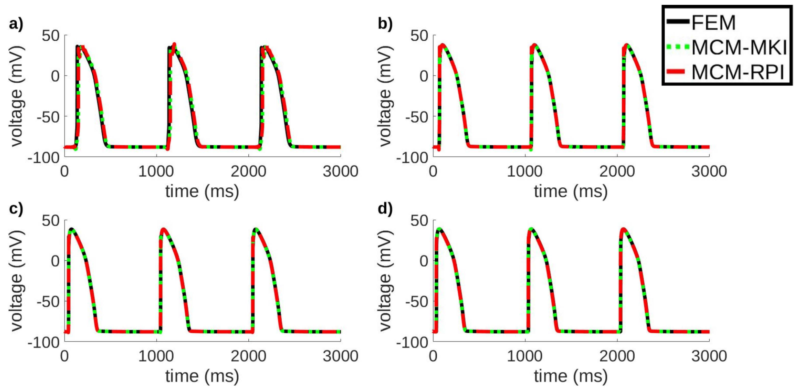
3.1. Electrical Propagation in a 2D Tissue Sheet

We considered a 5 × 5 cm human ventricular tissue sheet, where transmural heterogeneity was included by defining endocardial, midmyocardial, and epicardial regions in a 50:20:30 ratio. The cardiac fiber direction vector l was considered parallel to the x-axis. We used diffusion coefficient d 0 = 0.0013 cm 2 /ms and transversal-to-longitudinal conductivity ratio ρ = 0.2 . Stimuli with amplitude twice the diastolic threshold, period t T = 1 s, and duration t d = 1 ms were applied on the left side of the tissue ( x = 0 cm). The propagation of the action potential (AP) was simulated for a total time t s = 3 s.
We compared the MCM solution with RPI and MKI trial functions against FEM simulation results using bilinear isoparametric elements. We considered regular nodal discretizations and quadrilateral meshes with nodal spacing h = { 0.2 , 0.1 , 0.05 , 0.025 } cm. The considered support domains in the meshfree approximation had size s d = α s d h , with α s d = 2.8 . The generated APs at the center of the tissue sheet ( x = 2.5 cm, y = 2.5 cm) in the time interval t = [ 0 3 ] s for the different nodal spacing values are shown in Figure 1. We quantified the differences between MCM and FEM solutions in terms of mean transmembrane potential difference (TPD). Mean TPD between the FEM and the MCM with MKI trial functions was TPD = {3.111, 0.339, 0.401, 0.583} mV while mean TPD between the FEM and the MCM with RPI trial functions was TPD = {3.112, 0.340, 0.400, 0.582} mV for nodal spacing h = { 0.2 , 0.1 , 0.05 , 0.025 } cm. The efficiency of each simulation was evaluated in terms of execution time in Figure 2a.

3.2. Electrical Propagation in a 3D Tissue Slab

We investigated the effect of the support domain’s dilatation coefficient α s d by computing the normalized root mean square (NRMS) error between MCM and FEM solutions for a 3 × 3 × 3 cm tissue slab. The tissue was assumed to be composed of epicardial ventricular cells. Stimuli of amplitude twice diastolic threshold, period t T = 1 s, and duration t d = 1 ms were applied onto the left side of the tissue slab ( x = 0 cm). The tissue slab was discretized with h = 0.05 cm and varying dilatation coefficient α s d = { 2.25 , 2.50 , 2.75 , 3.00 , 3.25 , 3.50 } . The NRMS error was computed using the formula
NRMS = I = 1 N V M C M I V F E M I 2 N max I V F E M I min I V F E M I
where V M C M I and V F E M I denote the transmembrane potential value at node I computed with the MCM and the FEM, respectively. The NRMS error convergence plot is given in Figure 3.
The maximum NRMS error of the MCM solutions with RPI or MKI trial functions was obtained for α s d = 2.25 and was equal to 0.262 and 0.263, respectively. The minimum NRMS error was obtained for α s d = 3.5 and it was equal to 0.056 for RPI and 0.057 for MKI trial functions. The execution time for the simulations with varying dilatation coefficient is summarized in Figure 2b.

3.3. Electrical Propagation in the Niederer Benchmark Geometry

In this example, we evaluate our proposed method by solving the benchmark problem defined by Niederer et al., which is the standard, accepted approach to verify cardiac tissue electrophysiology simulators [35]. The benchmark problem considers a 3D cuboid of human ventricular tissue ( 3 × 7 × 20 mm). Cardiac fiber orientation is parallel to the Z axis and electrophysiology is described by the Ten Tusscher et al. model [36]. The longitudinal diffusion coefficient is set to d 0 = 0.00115 cm 2 /ms and the transverse-to-longitudinal ratio is ρ = 0.12 . Periodic stimulation with frequency f = 1 Hz, amplitude A = 50 mA and duration t d = 2 ms is applied at a cubic region with dimensions 1.5 × 1.5 × 1.5 mm located at corner P1 (Figure 4).
The activation time at the corners (P1 – P8) and the center (C) of the cuboid were computed for various nodal spacings, h = { 0.1 ,   0.2 ,   0.5 } mm, using MCM-RPI and MCM-MKI with support domain s d = α s d h , with α s d = 2.8 . Integration was performed using the DAETI method with time step d t = 0.1 ms. The activation times obtained by MCM-RPI and MCM-MKI were compared with those of the FEM (Table 1) previously reported in [33] and validated with the reported activation times in [35].

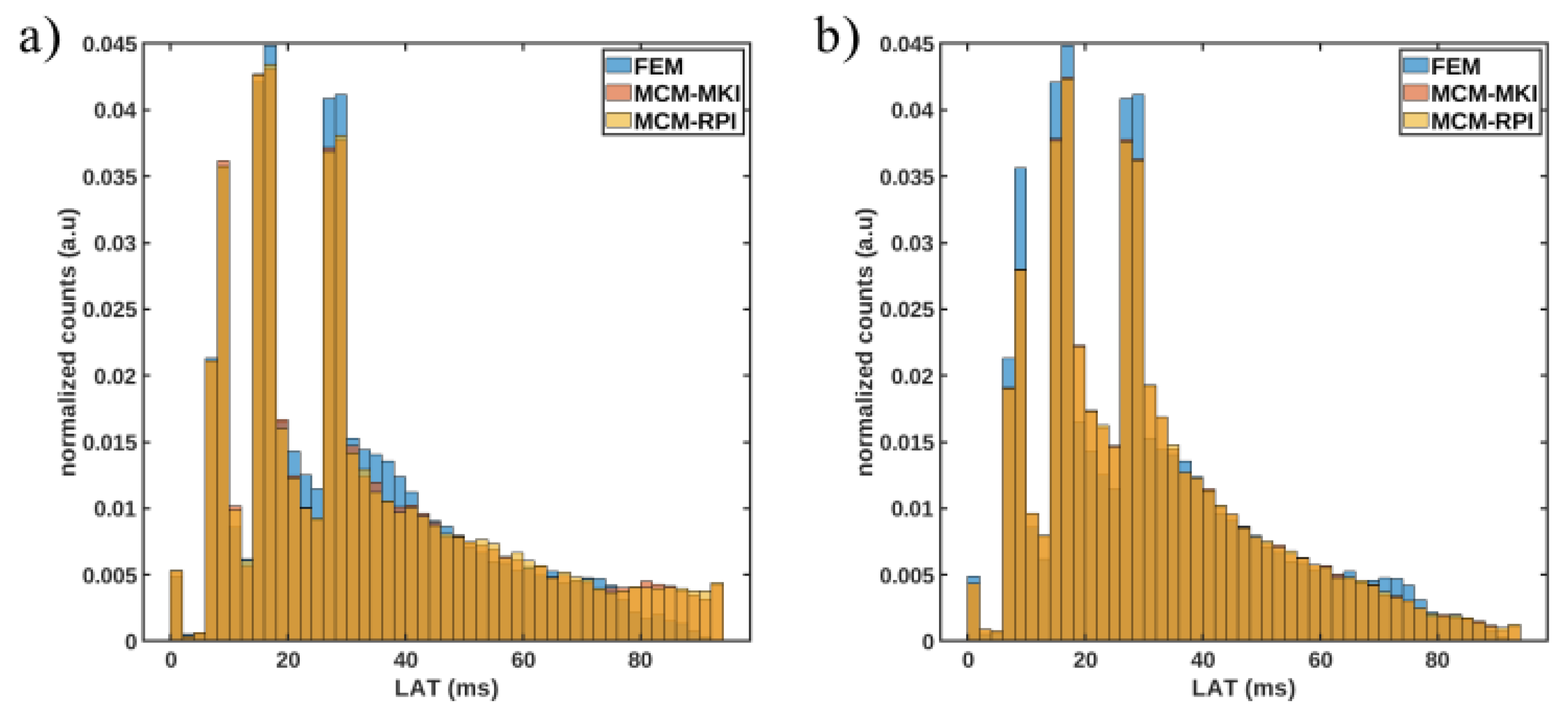
3.4. Electrical Propagation in 3D Biventricular Geometry with Irregular Nodal Distribution

We simulated electrical propagation in a porcine cardiac biventricular model under healthy conditions. The biventricular model was generated from the segmentation of a diffusion weighted-magnetic resonance image (DW-MRI) with dimensions 128 × 128 × 83 mm 3 and voxel size 1.09 × 1.09 × 1.2 mm 3 . Three labels were included in the segmentation to partition the ventricular wall in endocardial, midmyocardial, and epicardial regions with a 45:25:30 ratio. Median filter smoothing with 2 mm kernel size was applied on the segmentated data to ensure a smooth boundary. A tetrahedral mesh (69,621 nodes and 380,299 elements) was generated using the iso2mesh toolkit [37]. An irregular nodal distribution was obtained from the tetrahedral mesh of the DW-MRI segmentation.
The direction of myocardial fibers was obtained by computing the diffusion tensor (DT) field for each voxel of the DW-MRI. In brief, a linear minimum mean squared error (LMMSE) filter was applied to reduce Rician noise before computing the DT fields [38]. DT fields were computed by minimizing the Riemannian distance between an evaluated tensor spline and the DW-MRI data [39]. The principal eigenvector, which was obtained by solving the eigenvalue problem for the DT of each voxel, was considered as the myocardial fiber orientation of the corresponding voxel. The myocardial fiber orientations at the nodes of the tetrahedral mesh were obtained by interpolating the orientations of the image voxels using the MKI approximants.
Electrical propagation was simulated using a value for the diffusion coefficient of d 0 = 0.002 cm 2 /ms in the longitudinal direction of the myocardial fibers and a transverse-to-longitudinal conductivity ratio value of ρ = 0.15 . The electrophysiology of the ventricular myocardial tissue was represented by the O’Hara et al. model, as in previous examples. The points of earliest activation across the ventricles were identified by coupling the biventricular model with a network of Purkinje fibers generated using a fractal-tree generation algorithm [40]. We applied stimuli with t d = 1 ms, t T = 1 s, and amplitude twice the diastolic threshold onto the Purkinje–myocardial junctions (PMJs) which were identified from the terminal nodes of the Purkinje network. Electrical impulse propagation was simulated using the MCM with RPI and MKI approximants as well as the FEM for a simulation time t s = 150 ms.
Rather than constructing dilated support domains, we chose to construct support domains using the nearest-neighbor approach due to the irregular distribution of the nodes in the tetrahedral mesh. For such distributions, dilated support domains require the inclusion of a very large number of neighboring nodes to ensure numerical stability. In the nearest-neighbor approach, we used the 150 nearest nodes to accurately capture the steep voltage gradients of the monodomain model. The MCM solution with RPI approximants (MCM-RPI) and MKI approximants (MCM-MKI) was compared with the FEM in terms of local activation time (LAT) (see Figure 5). The mean local activation time was found to be 35.9 ms for MCM-RPI and 35.3 ms for MCM-MKI, while the mean LAT for FEM was 30.3 ms. To further evaluate LAT differences, we constructed the LAT normalized histogram (Figure 6a). We measured the normalized histogram intersection (NHI) as a metric of histogram similarity, which is given by the equation below:
N H I = i = 1 n m i n ( X i , Y i ) i = 1 n Y i ,
where i is the histogram bin index, n is the number of histogram bins, and X i and Y i denote the entry at the i t h bin of the normalized LAT histogram for the MCM and the FEM, respectively. NHI was found to be 0.937 for MCM-RPI and 0.939 for MCM-MKI. The execution time was 4.7 min for MCM-RPI, 4.6 min for MCM-MKI, and 6.1 min for FEM.

3.5. Electrical Propagation in 3D Biventricular Geometry with Immersed Grid Nodal Distribution

In this section, we simulate electrical propagation in the biventricular geometry using the same protocol as in Section 3.4. However, we perform the simulation with the MCM considering an immersed grid nodal distribution [41]. The immersed grid (70,027 nodes) was generated automatically by assigning field nodes at the center of the DW-MRI voxels. Field nodes were assigned only to the voxels that belonged to the segmentation of the biventricular anatomy. A point containment test algorithm [42] was used to discard nodes outside a triangular surface mesh representing the smooth boundary of the segmented biventricular anatomy. Consequently, the final immersed grid was composed of the nodes inside the biventricular model and the nodes on the boundary surface mesh of the model (Figure 7).
The mean LAT for the solution obtained by MCM-RPI was found to be 31.6 ms, while the mean LAT for MCM-MKI was 31.5 ms, both of them being very close to the mean LAT for FEM, which was 30.3 ms. The LAT maps are shown in Figure 8. As in Section 3.4, the normalized LAT histograms were computed for MCM-RPI and MCM-MKI. NHI was found to be 0.935 for MCM-RPI, and 0.936 for MCM-MKI. The normalized LAT histograms are given in Figure 6b. The execution time was 4.6 min for MCM-RPI and 4.4 min for MCM-MKI.

4. Discussion

In this study, we derived the mixed collocation method (MCM) to solve the monodomain model for the numerical simulation of cardiac electrophysiology. We considered two different interpolating trial functions, the radial point interpolation (RPI) and the moving kriging interpolation (MKI). We solved several numerical examples in 2D and 3D domains, comparing the MCM solution with a solution obtained by the FEM. The accuracy of MCM solutions was found to be similar for both RPI and MKI approximants. However, MKI was more efficient since, in contrast to RPI, it does not require polynomial enrichment. It should be noted that the optimal values of the parameters for the RPI and MKI approximations were obtained manually in this study. However, optimization techniques such as those based on minimizing a predictor function could be applied to obtain the values of these parameters automatically. For further details on the topic we refer the reader to [43].
In all the numerical examples in 2D tissue sheets and 3D tissue slabs, good agreement was found between MCM and FEM solutions. The convergence analysis in 3D tissue slabs demonstrated that the MCM solution improved for larger support domains as the number of included collocation points was increased (see Figure 3). However, as expected, as the size of the support domain increased, the execution time was also increased, as can be seen in Figure 2. Therefore, a compromise between accuracy and execution time must be made. The value α s d = 2.8 represents a good compromise. In the case of the biventricular anatomy model, including the 150 nearest neighbors of each field node in its support domain was found to be an optimal choice balancing accuracy and memory footprint. Local activation time (LAT) maps generated with the MCM were shown to be in good agreement with those obtained by the FEM. The mean LAT difference between the MCM and the FEM was reduced from 18% for irregular nodal distribution to 4% for immersed grid nodal distribution. Normalized histogram intersection with the FEM solution remained similar for both nodal distributions (over 0.93). These results, in combination with the simplicity of field nodes generation with the immersed grid approach, demonstrate an important advantage of the MCM over the FEM, especially for clinical applications where clinical image data could be treated directly as a meshfree model by the MCM, while the FEM requires the generation of a mesh. In addition, the FEM requires mesh preprocessing prior to the simulation to define parameters such as ventricular tissue partition and myocardial fiber orientation. The MCM with the immersed grid approach does not require any preprocessing since there is a one-to-one relationship between image voxels and field nodes. Anatomic partition data and myocardial fiber orientation defined on the voxels of the image are assigned directly to the corresponding immersed grid nodes. The flexibility of the MCM renders it a useful numerical method that could be extended to other applications, such as the investigation of soft tissue mechanical response [17].
In terms of execution efficiency, the simulation time for the MCM was comparable to the FEM for the 2D tissue sheet simulations. In the simulation of the biventricular anatomy model, the MCM presented better performance, with reductions in computational time of up to 28% compared to the FEM for both irregular and immersed grid nodal distributions. This was due to the size of the critical time step that was used during the adaptive explicit integration using the DAETI algorithm. In realistic models of complex geometry, such as the biventricular anatomy, small mesh elements restricting the size of the critical time step may arise. This limitation is relaxed when meshfree approximants are used. Therefore, the MCM presents higher efficiency despite the higher number of support domain nodes. For more information regarding the choice of the critical time step in DAETI, we refer the reader to [33].
The findings of this study support considering the MCM as a promising alternative to the FEM for cardiac electrophysiology simulation since its meshfree nature alleviates the need for the generation of a mesh and can, thus, allow fast model generation in a clinical setting together with an efficient simulation.

Author Contributions

Conceptualization, K.A.M. and E.P.; methodology, K.A.M. and E.P.; software, K.A.M.; validation, K.A.M. and E.P.; formal analysis, K.A.M.; investigation, K.A.M.; resources, E.P.; data curation, K.A.M.; writing—original draft preparation, K.A.M.; writing—review and editing, K.A.M. and E.P.; visualization, K.A.M.; supervision, E.P.; project administration, E.P.; funding acquisition, E.P. All authors have read and agreed to the published version of the manuscript.

Funding

This work was supported by Ministerio de Ciencia e Innovación (Spain) through projects PID2019-105674RB-I00, PID2022-140556OB-I00 and TED2021-130459B-I00, by European Social Fund (EU) and Aragón Government through project LMP94_21 and BSICoS group T39_23R, by European Research Council under G.A. 638284 and by EU H2020 Program under G.A. 874827 (BRAV∃).

Institutional Review Board Statement

Not applicable.

Informed Consent Statement

Not applicable.

Data Availability Statement

Data will be made available on request.

Conflicts of Interest

The authors declare no conflict of interest.

References

  1. Lopez-Perez, A.; Sebastian, R.; Ferrero, J.M. Three-dimensional cardiac computational modelling: Methods, features and applications. Biomed. Eng. Online 2015, 14, 35. [Google Scholar] [CrossRef] [PubMed]
  2. Niederer, S.A.; Lumens, J.; Trayanova, N.A. Computational models in cardiology. Nat. Rev. Cardiol. 2019, 16, 100–111. [Google Scholar] [CrossRef] [PubMed]
  3. Sampedro-Puente, D.A.; Raphel, F.; Fernandez-Bes, J.; Laguna, P.; Lombardi, D.; Pueyo, E. Characterization of spatio-temporal cardiac action potential variability at baseline and under β-adrenergic stimulation by combined unscented Kalman filter and double greedy dimension reduction. IEEE J. Biomed. Health Inform. 2020, 25, 276–288. [Google Scholar] [CrossRef] [PubMed]
  4. Rama, R.R.; Skatulla, S. Towards real-time cardiac mechanics modelling with patient-specific heart anatomies. Comput. Methods Appl. Mech. Eng. 2018, 328, 47–74. [Google Scholar] [CrossRef]
  5. Pueyo, E.; Dangerfield, C.; Britton, O.; Virág, L.; Kistamás, K.; Szentandrássy, N.; Jost, N.; Varró, A.; Nánási, P.P.; Burrage, K.; et al. Experimentally-based computational investigation into beat-to-beat variability in ventricular repolarization and its response to ionic current inhibition. PLoS ONE 2016, 11, e0151461. [Google Scholar] [CrossRef]
  6. Chabiniok, R.; Wang, V.Y.; Hadjicharalambous, M.; Asner, L.; Lee, J.; Sermesant, M.; Kuhl, E.; Young, A.A.; Moireau, P.; Nash, M.P.; et al. Multiphysics and multiscale modelling, data–model fusion and integration of organ physiology in the clinic: Ventricular cardiac mechanics. Interface Focus 2016, 6, 20150083. [Google Scholar] [CrossRef]
  7. Tung, L. A Bi-Domain Model for Describing Ischemic Myocardial DC Potentials. Ph.D. Thesis, Massachusetts Institute of Technology, Cambridge, MA, USA, 1978. [Google Scholar]
  8. Keener, J.P.; Sneyd, J. Mathematical Physiology: Systems Physiology. II; Springer: Berlin/Heidelberg, Germany, 2009. [Google Scholar]
  9. Potse, M.; Dubé, B.; Richer, J.; Vinet, A.; Gulrajani, R.M. A comparison of monodomain and bidomain reaction-diffusion models for action potential propagation in the human heart. IEEE Trans. Biomed. Eng. 2006, 53, 2425–2435. [Google Scholar] [CrossRef]
  10. Mirams, G.R.; Arthurs, C.J.; Bernabeu, M.O.; Bordas, R.; Cooper, J.; Corrias, A.; Davit, Y.; Dunn, S.J.; Fletcher, A.G.; Harvey, D.G.; et al. Chaste: An open source C++ library for computational physiology and biology. PLoS Comput. Biol. 2013, 9, e1002970. [Google Scholar] [CrossRef]
  11. Vigmond, E.J.; Hughes, M.; Plank, G.; Leon, L.J. Computational tools for modeling electrical activity in cardiac tissue. J. Electrocardiol. 2003, 36, 69–74. [Google Scholar] [CrossRef]
  12. Lluch, È.; De Craene, M.; Bijnens, B.; Sermesant, M.; Noailly, J.; Camara, O.; Morales, H.G. Breaking the state of the heart: Meshless model for cardiac mechanics. Biomech. Model. Mechanobiol. 2019, 18, 1549–1561. [Google Scholar] [CrossRef]
  13. Lluch, E.; Doste, R.; Giffard-Roisin, S.; This, A.; Sermesant, M.; Camara, O.; De Craene, M.; Morales, H.G. Smoothed particle hydrodynamics for electrophysiological modeling: An alternative to finite element methods. In Proceedings of the International Conference on Functional Imaging and Modeling of The Heart, Toronto, ON, Canada, 11–13 June 2017; pp. 333–343. [Google Scholar]
  14. Zhang, H.; Ye, H.; Huang, W. A meshfree method for simulating myocardial electrical activity. Comput. Math. Methods Med. 2012, 2012, 936243. [Google Scholar] [CrossRef] [PubMed]
  15. Mountris, K.A.; Sanchez, C.; Pueyo, E. A novel paradigm for in silico simulation of cardiac electrophysiology through the Mixed Collocation Meshless Petrov-Galerkin Method. In Proceedings of the 2019 Computing in Cardiology (CinC), Singapore, 8–11 September 2019; p. 1. [Google Scholar]
  16. Legner, D.; Skatulla, S.; MBewu, J.; Rama, R.; Reddy, B.; Sansour, C.; Davies, N.; Franz, T. Studying the influence of hydrogel injections into the infarcted left ventricle using the element-free Galerkin method. Int. J. Numer. Methods Biomed. Eng. 2014, 30, 416–429. [Google Scholar] [CrossRef] [PubMed]
  17. Zhang, G.; Wittek, A.; Joldes, G.; Jin, X.; Miller, K. A three-dimensional nonlinear meshfree algorithm for simulating mechanical responses of soft tissue. Eng. Anal. Bound. Elem. 2014, 42, 60–66. [Google Scholar] [CrossRef]
  18. Belytschko, T.; Lu, Y.Y.; Gu, L. Element-free Galerkin methods. Int. J. Numer. Methods Eng. 1994, 37, 229–256. [Google Scholar] [CrossRef]
  19. Mountris, K.A.; Bourantas, G.C.; Millán, D.; Joldes, G.R.; Miller, K.; Pueyo, E.; Wittek, A. Cell-based maximum entropy approximants for three-dimensional domains: Application in large strain elastodynamics using the meshless total Lagrangian explicit dynamics method. Int. J. Numer. Methods Eng. 2020, 121, 477–491. [Google Scholar] [CrossRef]
  20. Chen, J.; Beraun, J.; Carney, T. A corrective smoothed particle method for boundary value problems in heat conduction. Int. J. Numer. Methods Eng. 1999, 46, 231–252. [Google Scholar] [CrossRef]
  21. Bonet, J.; Lok, T.S. Variational and momentum preservation aspects of smooth particle hydrodynamic formulations. Comput. Methods Appl. Mech. Eng. 1999, 180, 97–115. [Google Scholar] [CrossRef]
  22. Atluri, S.N. The Meshless Method (MLPG) for Domain and BIE Discretizations; Tech Science Press: Henderson, NV, USA, 2004; p. 677. [Google Scholar]
  23. Atluri, S.N.; Shen, S. The basis of meshless domain discretization: The meshless local Petrov-Galerkin (MLPG) method. Adv. Comput. Math. 2005, 23, 73–93. [Google Scholar] [CrossRef]
  24. Libre, N.; Emdadi, A.; Kansa, E.; Rahimian, M.; Shekarchi, M. A stabilized RBF collocation scheme for Neumann type boundary value problems. Comput. Model. Eng. Sci. 2008, 24, 61–80. [Google Scholar]
  25. Atluri, S.N.; Liu, H.T.; Han, Z.D. Meshless local Petrov-Galerkin (MLPG) mixed collocation method for elasticity problems. Comput. Model. Eng. Sci. 2006, 4, 141. [Google Scholar]
  26. Lancaster, P.; Salkauskas, K. Surfaces generated by moving least squares methods. Math. Comput. 1981, 37, 141–158. [Google Scholar] [CrossRef]
  27. Wang, J.; Liu, G. A point interpolation meshless method based on radial basis functions. Int. J. Numer. Methods Eng. 2002, 54, 1623–1648. [Google Scholar] [CrossRef]
  28. Mountris, K.A.; Pueyo, E. The radial point interpolation mixed collocation method for the solution of transient diffusion problems. Eng. Anal. Bound. Elem. 2020, 121, 207–216. [Google Scholar] [CrossRef]
  29. Gu, L. Moving kriging interpolation and element-free Galerkin method. Int. J. Numer. Methods Eng. 2003, 56, 1–11. [Google Scholar] [CrossRef]
  30. Qu, Z.; Garfinkel, A. An advanced algorithm for solving partial differential equation in cardiac conduction. IEEE Trans. Biomed. Eng. 1999, 46, 1166–1168. [Google Scholar]
  31. Hundsdorfer, W.; Verwer, J.G. Numerical Solution of Time-Dependent Advection-Diffusion-Reaction Equations; Springer Science & Business Media: Berlin/Heidelberg, Germany, 2007; Volume 33. [Google Scholar]
  32. Overvelde, J.T. The Moving Node Approach in Topology Optimization. Master’s Thesis, Delft University of Technology, Delft, The Netherlands, 2012. [Google Scholar]
  33. Mountris, K.A.; Pueyo, E. A dual adaptive explicit time integration algorithm for efficiently solving the cardiac monodomain equation. Int. J. Numer. Methods Biomed. Eng. 2021, 37, e3461. [Google Scholar] [CrossRef]
  34. O’Hara, T.; Virág, L.; Varró, A.; Rudy, Y. Simulation of the undiseased human cardiac ventricular action potential: Model formulation and experimental validation. PLoS Comput. Biol. 2011, 7, e1002061. [Google Scholar] [CrossRef]
  35. Niederer, S.A.; Kerfoot, E.; Benson, A.P.; Bernabeu, M.O.; Bernus, O.; Bradley, C.; Cherry, E.M.; Clayton, R.; Fenton, F.H.; Garny, A.; et al. Verification of cardiac tissue electrophysiology simulators using an N-version benchmark. Philos. Trans. R. Soc. A Math. Phys. Eng. Sci. 2011, 369, 4331–4351. [Google Scholar] [CrossRef]
  36. Ten Tusscher, K.H.; Panfilov, A.V. Alternans and spiral breakup in a human ventricular tissue model. Am. J. Physiol.-Heart Circ. Physiol. 2006, 291, H1088–H1100. [Google Scholar] [CrossRef]
  37. Fang, Q.; Boas, D.A. Tetrahedral mesh generation from volumetric binary and grayscale images. In Proceedings of the 2009 IEEE International Symposium on Biomedical Imaging: From Nano to Macro, Boston, MA, USA, 28 June–1 July 2009; pp. 1142–1145. [Google Scholar]
  38. Tristán-Vega, A.; Aja-Fernández, S. DWI filtering using joint information for DTI and HARDI. Med Image Anal. 2010, 14, 205–218. [Google Scholar] [CrossRef]
  39. Barmpoutis, A.; Vemuri, B.C. A unified framework for estimating diffusion tensors of any order with symmetric positive-definite constraints. In Proceedings of the 2010 IEEE International Symposium on Biomedical Imaging: From Nano to Macro, Barcelona, Spain, 2–5 May 2010; pp. 1385–1388. [Google Scholar]
  40. Costabal, F.S.; Hurtado, D.E.; Kuhl, E. Generating Purkinje networks in the human heart. J. Biomech. 2016, 49, 2455–2465. [Google Scholar] [CrossRef] [PubMed]
  41. Mountris, K.A.; Pueyo, E. Next-generation In Silico Cardiac Electrophysiology Through Immersed Grid Meshfree Modeling: Application To Simulation Of Myocardial Infarction. In Proceedings of the 2020 Computing in Cardiology, Rimini, Italy, 13–16 September 2020; pp. 1–4. [Google Scholar]
  42. Liu, J.; Chen, Y.; Maisog, J.M.; Luta, G. A new point containment test algorithm based on preprocessing and determining triangles. Comput.-Aided Des. 2010, 42, 1143–1150. [Google Scholar] [CrossRef]
  43. Mongillo, M. Choosing basis functions and shape parameters for radial basis function methods. SIAM Undergrad. Res. Online 2011, 4, 2–6. [Google Scholar] [CrossRef]
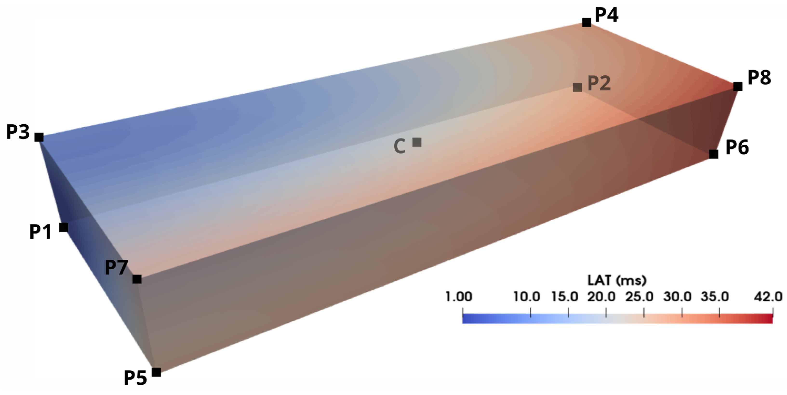
Figure 1. Voltage traces at the center ( x = 2.5 cm, y = 2.5 cm) of a 5 × 5 cm ventricular tissue sheet calculated using the FEM (continuous black), the MCM with MKI (dotted green), and the MCM with RPI (dashed red). The nodal discretization spacing is (a) h = 0.2 cm, (b) h = 0.1 cm, (c) h = 0.05 cm, and (d) h = 0.025 cm.
Applsci 13 11460 g001
Figure 2. Execution time for (a) varying spacing in a 5 × 5 cm tissue sheet and (b) varying support dilatation coefficient in a 3 × 3 × 3 cm tissue slab. Execution time is reported for the FEM (black), the MCM with MKI trial functions (blue), and the MCM with RPI trial functions (red).
Applsci 13 11460 g002
Figure 3. Convergence rate for varying support domain’s dilatation coefficient α s d { 2.25 , 2.50 , 2.75 , 3.00 , 3.25 , 3.50 } for the MCM with MKI (continuous blue) and RPI (slashed red) trial functions. Convergence is evaluated by computing the NRMS error with respect to an FEM simulation.
Applsci 13 11460 g003
Figure 4. Local activation time (LAT) map for the MCM-MKI solution of the Niederer benchmark [35] with space discretization h = 0.1 mm.
Applsci 13 11460 g004
Figure 5. Local activation time maps for FEM (left), MCM-RPI (center), and MCM-MKI (right) simulations in a biventricular model with irregular nodal distribution.
Applsci 13 11460 g005
Figure 6. Local activation time histogram comparison for MCM simulation with RPI approximants (MCM-RPI) or MKI approximants (MCM-MKI) and FEM. (a) Irregular nodal distribution. (b) Immersed grid nodal distribution.
Applsci 13 11460 g006
Figure 7. Immersed grid model generation. (a) The boundary surface mesh is extracted from the tetrahedral biventricular mesh. (b) Nodes are assigned at the image data voxels. (c) Nodes located outside the surface mesh are discarded using a point containment test.
Applsci 13 11460 g007
Figure 8. Local activation time maps for FEM (left), MCM-RPI (center), and MCM-MKI (right) simulations on an immersed grid of the biventricular model. Nonconductive connective tissue is represented in yellow.
Applsci 13 11460 g008
Table 1. Activation times at the corners (P1–P8) and the center (C) of the 3D cuboid benchmark problem.
h (mm)P1P2P3P4P5P6P7P8C
MCM-RPI activation time (ms)
0.515123599911510712056
0.213411363753425826
0.1130833294231442
MCM-MKI activation time (ms)
0.514924609911110111958
0.213312363655395526
0.1130832294231422
FEM activation time (ms)
0.51492258941099811154
0.213111353551395425
0.11298312741294120
Disclaimer/Publisher’s Note: The statements, opinions and data contained in all publications are solely those of the individual author(s) and contributor(s) and not of MDPI and/or the editor(s). MDPI and/or the editor(s) disclaim responsibility for any injury to people or property resulting from any ideas, methods, instructions or products referred to in the content.

