Abstract
One of the fundamental challenges in geophysics is the calculation of distribution models for physical properties in the subsurface that accurately reproduce the measurements obtained in the survey and are geologically plausible in the context of the study area. This is known as inverse modeling. Performing a 3D joint inversion of multimodal geophysical data is a computationally intensive task. Additionally, since it involves a modeling process, finding a solution that matches the desired characteristics requires iterative calculations, which can take days or even weeks to obtain final results. In this paper, we propose a robust numerical solution for 3D joint inversion of gravimetric and magnetic data with Gramian-based structural similarity and structural direction constraints using parallelization as a high-performance computing technique, which allows us to significantly reduce the total processing time based on the available Random-Access Memory (RAM) and Video Random-Access Memory (VRAM)and improve the efficiency of interpretation. The solution is implemented in the high-level programming languages Fortran and Compute Unified Device Architecture (CUDA) Fortran, capable of optimal resource management while being straightforward to implement. Through the analysis of performance and computational costs of serial, parallel, and hybrid implementations, we conclude that as the inversion domain expands, the processing speed could increase from 4× up to 100× times faster, rendering it particularly advantageous for applications in larger domains. We tested our algorithm with two synthetic data sets and field data, showing better results than standard separate inversion. The proposed method will be useful for joint geological and geophysical interpretation of gravimetric and magnetic data used in exploration geophysics for example minerals, ore, and petroleum search and prospecting. Its application will significantly increase the reliability of physical-geological models and accelerate the process of data processing.
1. Introduction
Geophysical methods are one of the main ways to study the Earth’s crust and search and explore the mineral resources in the Earth’s interior [1,2,3]. Geophysical methods can be classified based on the physical fields used in their application. Gravity and magnetic methods thus belong to the so-called potential methods of geophysics since they are based on potential theory [4,5,6,7].
One of the fundamental challenges in geophysics is the calculation of distribution models of physical properties in the subsurface that can accurately reproduce measurements obtained in the field, in turn, these models are geologically possible in the context of the study area, which is known as inverse modeling. Any inversion problem is subject to three constraints: (1) the solution must exist, (2) the process is unstable, and (3) the solution is not unique [4,8,9,10,11].
The informativeness and reliability of the interpretation of geophysical data depend greatly on the method of their inversion. Many studies have been devoted to this topic; we will briefly try to summarize different techniques of joint inversion, their advantages, and their disadvantages. At the same time, it is important to realize that the inversion of different methods may differ in the mathematical apparatus used for their joint processing.
For example, in petrophysical inversion [12,13], a reliable result can be achieved using Newton–Gauss iteration [14]. The authors note that separate inversion of electromagnetic or seismic data is highly ambiguous and leads to great ambiguity in determining porosity and fluid saturation. Using the Gauss-Newton algorithm equipped with multiplicative regularization and a proper data-weighting scheme in the example with real data, the authors showed that up to 20% errors in the saturation and porosity exponents in Archie’s equations do not cause significant errors in the inversion results [12,13].
Spichak [15] in his work on this topic points out that in petrophysical data inversion, it is necessary to apply two levels of initial data, the accuracy and representativeness of which influence the final result. Lelievre [16] introduced so-called weight coefficients (regularization terms) for this purpose. As a result, when applying this type of joint inversion, it is necessary to introduce two regularization levels. Level 1 (conductivity, seismic velocity, and density) and Level 2 (porosity and water content). The disadvantage of this approach is that a lack of accuracy or number of measurements of Level 1 parameters will result in an unreliable inversion as a whole.
Franz et al. [17] analyze the compatibility of different methods in the joint inversion of geophysical data in a study of the Namibian continental margin. They note that electrical resistivity models obtained by inversion of marine data at shallow water depths are characterized by poor resolution for lithologic boundaries. To address this important problem, the authors use a joint inversion of magnetotelluric, gravimetric (fixed structural density model coupling with satellite gravity data), and seismic (fixed gradient velocity model) data. The number of iterations varies from 283 to 380; the Final MT and gravity data RMS are 3.01 and 1.52, respectively.
In turn, Gallardo & Meju [18] proposed a joint inversion of magnetotelluric and seismic data, applying this method to the interpretation of geologic features such as sedimentary basins, crustal and upper mantle structures, oil reservoirs, etc. The joint inversion of these data with added noise has led to good results, but its numerical implementation is often unstable and requires regularization [15]. The main disadvantage of this method is the need for structural semblance of the models and too much computer core memory, especially for three-dimensional inversion.
It is important to note that inversion can be interactive or sequential. Dell’Aversana [19,20] describes this process in detail, using the construction of a velocity model following a tomographic inversion. If necessary, the new seismic section is further used to simulate resistivity, etc. The approach is advantageous as it is relatively simple and requires much less computer core memory than the simultaneous joint inversion [15].
According to Reimann et al. [21], inversion methods can be categorized as follows: Cluster analysis is grouping according to the proximity of samples in the space of properties [22,23]; the Gaussian classifier is based on the assumption that the vector of properties has an n-dimensional Gaussian distribution of the conditional pdf within each lithological group [23]; K-means clustering implies an iterative search of a set of points (centers) so as to minimize the mean squared distance from each data point to its nearest center in training samples [24]; Discriminant analysis searches the functions of properties that separate groups in an optimal way (in terms of root mean square) in order to choose the combination of linear coefficients to maximize the variance of group centroids while minimizing the variance within the groups [25].
In this regard, the approach of the objective function according to the type of problem to be solved and the way to obtain a solution are fundamental to achieving satisfactory results; thus, a mathematical approach to obtain a solution capable of fitting the needs of each particular case is what we call “robust”. The evaluation of uncertainty is an important step in inversion [26] since inverse problems always belong to decision-making processes and, by nature, are ill-posed, i.e., there are different solutions (called equivalents) that are compatible with the prior information and fit the observed data within the same error bounds [11,27,28,29].
The main objective of geophysical data inversion, and in this case, gravity and magnetic data, is to solve the inverse problem of geophysics and related geological problems. Such problems include geologic structure, tectonics and geodynamics, volcanism and seismic processes, hydrogeology and mineral resource studies, etc. The advantages of these methods are relatively low cost, high productivity of work, and the possibility to obtain information about large territories in great depth. Many examples of successful applications of potential methods in different areas of the world and for solving both prospecting and theoretical geologic problems are described [30,31,32]. In the first stages, the inversion of geophysical data is carried out in two dimensions and for each method separately [33,34,35,36,37,38]. The next step may be three-dimensional modeling [39,40]. The last step may be a joint inversion by two or more methods, performed in two and three dimensions [41,42,43]. A serious disadvantage of gravity and geomagnetic methods is the ambiguity of the interpretation of the obtained data. Beyond the reductions as such, data analysis, functional fitting, and regional-local anomaly separation will also introduce errors; however, these remain essentially undefined because the basic assumptions are arbitrary and regional-local separation as such cannot be made in an unambiguous manner [44,45,46]. It should be noted that this is a problem for most geophysical methods. One way to overcome this problem, or at least to reduce uncertainty about the results, is to apply different filters and integrate methods [47,48]. However, this is not always successful either. The best results can currently be achieved by the joint inversion of several methods, significantly improving the reliability of the interpretation [49,50,51,52,53]. On the other hand, it makes the mathematical procedure of data processing more complex and leads to the need for higher time consumption and more computational power; high-performance computing techniques are an important task to improve the mathematical process of joint data processing in order to obtain solutions in a reasonable time with ordinary personal computers.
High-performance computing (HPC) techniques to obtain solutions to inversion problems have been used since the late 1980s, as mentioned before [54]. However, starting in the second decade of the 2000s, a new era of HPC has developed thanks to the arrival of the new graphic processing units (GPU), its high parallelization capacity, and easy access outside the business or academic field due to its low cost. The most commonly used techniques in geophysics have focused mainly on electromagnetic and seismic methods and can be generally classified as parallelization of numerical methods [55,56,57,58,59,60,61], based on neural networks and deep learning [62,63,64,65], and more recently, based on quantum computing [66].
In this case, the variational modeling approach has been employed to construct an objective function or parametric functional consisting of (1) a mismatch term measuring the distance between and y, usually via the L2 norm, and (2) a regularization functional favoring appropriate minimizers and penalizing potential solutions with undesirable structures [67] using the form:
The regularization functional represents a family of linear operators that should stabilize the problem and bound desirable solutions within the infinite space of possible solutions, while is a scalar called the regularization parameter that gives weight to the regularization functional. The higher this value, the more influence it has on the solution; conversely, the closer to zero this value is, the closer it is to a solution without regularization. The purpose of regularization tools is to provide the user with easy-to-use routines based on numerically robust and efficient algorithms for doing experiments with regularization of discrete, ill-posed problems [68]. Two widely used regularizers are the Laplacian, which adds smoothness to the models because it is known that (general) changes in properties occur gradually; therefore, smoothed distributions are expected. On the other hand, sometimes there is subsurface information obtained directly or indirectly in previous studies, and the solution should incorporate such information, so an a priori model is used as a second regularizer. In addition, it is possible to know the predominant orientations of structures in the study area and some directional preference regularizer may be useful; therefore, the implementation of such regularizers allows robust solutions capable of fitting a wide variety of needs according to geological-structural context.
Joint inversion as a regularizer to mitigate the non-uniqueness of solutions has proven to be very effective [69,70,71,72,73,74,75,76]. This assumes that information obtained from different methods, whether directly or indirectly, comes from the same source interacting with different physical fields. Therefore, it is reasonable to expect inversion results where the distribution of different physical properties in the subsurface of the same study area have some relationship, as well as to propose the generation of models that feedback through each other through correspondence relationships that can be (1) intrinsic to rock physics or (2) structural. Zhdanov et al. [73] shows that in a Gramian space, the norm is a function that provides a measurement of the correlation between that function and the different parameters of the model within a Gram matrix. Due to its quadratic form similar to the L2 norm, it can be used as a regularizer of structural similarity, with the advantage that this function is differentiable, thus avoiding resorting to some linearization as in the case of crossed gradients [41].
To perform a 3D inversion of multiple types of geophysical data together is a task with an extremely high computational cost that grows exponentially as the resolution of the solutions increases. Furthermore, since it is a modeling process, finding a solution that meets the desired characteristics involves calculating solutions iteratively, which can take several days or weeks to obtain a final result.
In this work, we propose a robust numerical solution for 3D joint inversion for gravimetric and magnetic data using Gramian-based structural similarity and greater structural direction constraints, using parallelization as a high-performance computing technique, which allows us to significantly increase the processing speed and improve the efficiency of interpretation.
2. Methods
This methodology describes a 3D joint inversion for gravimetric and magnetic data with smoothness, a priori information, directional preference, and Gramian-based structural similarity constraints.
2.1. Regularized Least Squares 3D Joint Inversión with Gramian-Based Constraint
The following parametric functional expressed in its matrix form was used to make joint inversions of two types of geophysical data:
This is composed of the mismatch functional , a smoothing regularizer , an a priori model approximation regularizer , a structural direction regularizer , a verticality regularizer and the structural coupling regularizer using Gramian G(∇m, ∇m). Each of the elements represents the concatenated vectors and matrices of each input data type; in this case, gravimetric (1) and magnetic (2) data.
where I is an identity matrix, A is the linear operator for the direct modeling of gravimetry and magnetometry respectively, m is the vector encoding the model parameters or physical property distribution of a 3D domain (subsurface), d0 is the vector containing the measured data in a 2D domain (surface), mapr is the vector containing a priori information about the distribution of properties in the subsurface, Wd is the weights diagonal matrix of inverse standard deviation assigned to each data and Wm is the weights diagonal matrix of inverse standard deviation assigned to each cell in the model.
The regularization parameters determine the weight of the regularization functionals, which allows varying importance to be given to the regularizers in the inversion solutions for each specific case, thus having more control over the geometries of the contrasts obtained in the inversion models, thereby leaving the freedom to choose what kind of results are expected to the user’s objectivity.
The linear operators L, M, and N correspond to the Laplacian which smoothes the distribution of properties in the solutions, , which is the directional derivative of the strike θ and pitch ϕ angles and whose function is to specify a preferential structural direction, as well as the vertical derivative which depending of its regularization parameter sign favors vertical or horizontal properties distributions in the subsurface. These matrices were computed from the linearization of the 3D domain and discrete numerical derivatives using central differences and forward and backward differences depending on which position of each node in the 3D domain (Figure 1). This allowed us to obtain the curvature and derivatives of the domain without the need to consider extra cells or reduce the domain.
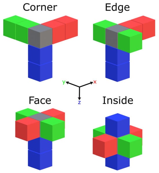
Figure 1.
3D mesh illustrating the cells involved in the computation of discrete numerical derivatives depending on the position of the central node.
The operators A(1) and A(2) were calculated using analytical solutions for straight prisms following the development of [77,78] for gravimetry and magnetometry, respectively (See Appendix A).
The Gramian [73] is defined as the determinant of the Gram matrix for the elements m(1) and m(2). The equivalence of the Gramian with respect to the L2 norm of crossed gradients is detailed in Appendix B of [76].
From Equation (2), we obtain Euler’s equation, which expresses the parameters m at which the parametric functional reaches a minimum (See Appendix B):
Regrouping the terms of Equation (6) as follows will be useful for their computational implementation:
where:
Details of the expressions are given in Appendix C.
2.2. Gravity and Magnetic Inversion Using Conjugate Gradient Algorithm
The following functional was proposed to be minimized through an iterative process to approximate the solution using the conjugate gradient method:
Thus, summarizing the iterative scheme is defined as follows:
where the stopping conditions will be (1) the maximum number of iterations and (2) the minimum misfit error achieved, both configured at the beginning of the process.
2.3. Coding Guidelines
For the computational implementation, memory management, the number of calculations to be performed, and the size of the arrays involved in operations were considered important points to optimize and achieve better performance. The Fortran 2008 standard [79] was used as the programming language because (1) it allowed the management of the memory size used by each array in a simple way, (2) also allowed to implement of the parallelization of matrix-vector type multiplications through the recently (2021) released free Compute Unified Device Architecture (CUDA) Fortran libraries within the Nvidia Corporation (NVIDIA) (Santa Clara, CA, USA) high-performance computing software development kit (HPC SDK v23.9), (3) as well as better performance compared to other high-level programming languages without complicating its parallel programming thanks to the similar syntax between the language and the parallelization library in contrast with other low-level programming languages. CUDA is a general parallel computing library developed by NVIDIA, which is a powerful tool compatible with popular programming languages.
Although it is convenient to process with concatenated arrays and vectors to describe the procedure, it was decided to perform the calculations of each type of geophysical data separately. This allowed to reduce the size of all the matrices to be multiplied by 50% since 2/4 parts of the concatenated matrices are filled with zeros. This implied performing a larger number of operations, but smaller in size, allowing faster processing and using a smaller amount of memory to store the temporary arrays. Even with these considerations, the memory usage and processing time grow exponentially as the inversion domain increases, depending on the number of cells to be processed and not on their dimensions.
In order to take full advantage of the computational power available during the modeling process, three different routines were programmed: A single-core version on the Central Processing Unit (CPU) with the amount of RAM available as the only limiting factor for the inversion domain size at the request of very long processing times, which has been compiled with two different compilers, gfortran and nvfortran, and showed consistently to be at least 4× times faster (Table 1). A parallel version that uses the Graphics processing unit (GPU) to perform all matrix-vector multiplications in the process in parallel, which is many times faster at the cost of relying on the amount of available VRAM memory, a much more difficult computational resource to obtain in large quantities. Finally, a CPU-GPU hybrid version aims to be a balance between speed and resource usage by performing only the calculations of structural similarity regularizer in parallel. Table 1 summarizes the performance of different processing routines for different inversion domain sizes based on RAM usage, VRAM usage, processing time, and how many times faster it is compared to the slower single-core version. Meanwhile, a visual comparison is presented in Figure 2. Performance tests were conducted on an easy to access desktop hardware (CPU: Ryzen 5 3600 3.95 GHz, GPU: NVIDIA 2060 super with 2176 CUDA cores and 8 GB VRAM; Memory: 2 × 16 GB), and processing times may vary in a different setup.

Table 1.
Table of computational performance of the different processing routines.
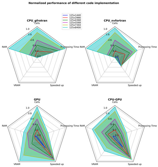
Figure 2.
Radar chart of Table 1 normalized values, highlighting the advantages and disadvantages of each routine as the inversion domain increases.
3. Results and Validation
To demonstrate the capabilities of a more robust parametric functional (Equation (2)), a comparison of results with respect to the standard separate inversion functional (Equation (17)) was performed:
The following expressions [80] were used to evaluate the RMS of normalized residuals and the model convergence for each iteration for each data type:
For gravimetric data when and magnetic data when and where is the covariance matrix associated with the data, n is the number of records corresponding to each type of geophysical data and ε is a small positive arbitrary value to avoid division by zero.
3.1. Synthetic Test Model 1
To validate the correct operation of the parametric functional, a synthetic experiment proposed by [81,82] was replicated, consisting of a dike inclined at 45 degrees and buried at 50 m deep in a half-space of zero contrast, with constant density and magnetization of 1 g/cm3 and 1 A/m, respectively. This model is made up of 20 × 20 × 10 (4000) voxels of 50 m per side, forming a volume of 1000 × 1000 × 500 cubic meters (Figure 3), from which gravity and magnetic anomalies were calculated by direct modeling, obtaining maps of 20 × 20 cells (400 data points) separated each 50 m and contaminated by Gaussian noise with a standard deviation of 2% to verify the sensitivity to noise of the inversion solutions. For the magnetic case, a field strength , I = 45° and D = 45° was considered. Figure 4 shows the resulting gravimetric and magnetic anomalies that were used as input data for the inverse modeling.
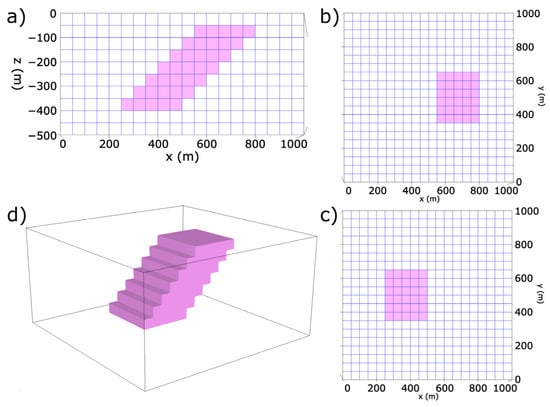
Figure 3.
Synthetic model of an inclined dike of 1 g/cm3 in density and 1 A/m in magnetization buried at a depth of 50 m in a homogeneous bottom of zero contrast, (a) profile, (b) plan section at 50 m depth, (c) plan section at 400 m depth and (d) 3-D view of the buried dike.
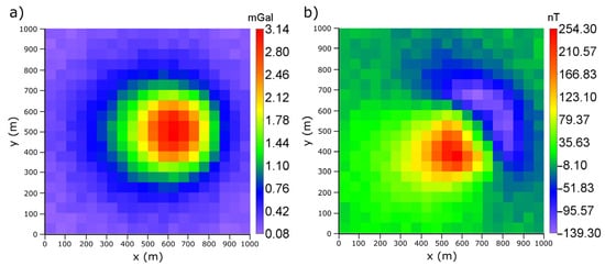
Figure 4.
(a) Gravity anomaly (mGal) and (b) magnetic anomaly (nT) produced by buried dike model in Figure 3. The data were contaminated with Gaussian noise of 2% of the standard deviation in order to test the noise sensitivity of the inversion solutions.
Standard Separate versus Robust Joint Inversion Results of Test Data 1
This experiment was performed with data contaminated by Gaussian noise to consider its effect on the inversion results. We considered hypothetical clipping information from two wells with real density values as a priori information for the gravity case the Well_1 at 350–400 m and Well_2 at 650–700 m on the x-axis in order to evaluate how the magnetic case improves with joint inversion. 40 iterations were run, and the stopping condition was convergence between models of less than 1%. The regularizers shared in standard separate (Equation (17)) and robust joint inversion functional (Equation (2)) were kept constant. For the joint inversion case, the “structural direction” regularizer was also used to indicate the strike and dip angles of the structure. Table 2 specifies the rest of the inversion parameters.
Table 2.
Inversion parameters for separate and joint inversion.
The results of the experiment at epoch 30 are plotted in Figure 5 with a general color scale ranging from 0 to 1 g/cm3 and A/m for the gravimetric and magnetic cases, respectively. Figure 6 also plots the model convergence of each iteration in percentage, which represents how much a model changes with respect to the past iteration and the RMS error of normalized residuals, which reflects the mismatch between the input synthetic data and the data calculated from the inversion models of each iteration.
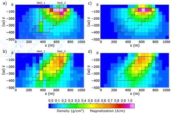
Figure 5.
Profiles of inversion results sliced at 500 m in y axis. Density distribution models (g/cm3) for (a) standard separate inversion, (b) our robust joint inversion. Magnetization distribution (A/m) for (c) standard separate inversion and (d) our robust joint inversion. Black markers represent the original position of buried dike and red markers represent Well location used as a priori information.
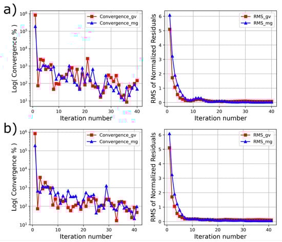
Figure 6.
Model convergence (Equation (18)) and data misfit (Equation (19)) were achieved in inversion of test data 1 at each iteration, (a) for standard separate inversion and (b) for our robust joint inversion.
We have shared access to an alpha version of the program under development at supplementary materials section where this synthetic model can be reproduced. All needed instructions are found within the repository description.
3.2. Synthetic Test Model 2
A second test model with bodies in different positions and property contrast, inspired by the synthetic models of [61,83], was used to further test the operation of the proposed parametric function in more complex situations. It is made of 30 × 20 × 15 (9000) voxels of 50 m per side, forming a volume of 1500 × 1000 × 750 cubic meters (Figure 7), from which gravity and magnetic anomalies were calculated by forward modeling, obtaining maps of 30 × 20 cells (600 data points) separated by 50 m; also, these maps were contaminated with Gaussian noise with a standard deviation of 5%. For the magnetic case, a field strength , I = 45° and D = 15° was considered. Figure 8 shows the resulting gravimetric and magnetic anomalies that were used as input data for the inverse modeling.
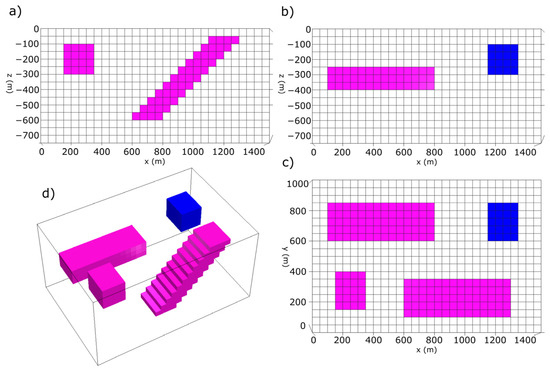
Figure 7.
Synthetic test model 2 of simple geometric buried bodies with +1 g/cm3 density contrast, +1 A/m magnetization contrast (rose bodies) and −1 g/cm3 density contrast, −1 A/m magnetization contrast (blue body). (a) profile view at y = 250 m, (b) profile view at y = 700 m, (c) top view at z = 0 m and (d) 3D view.
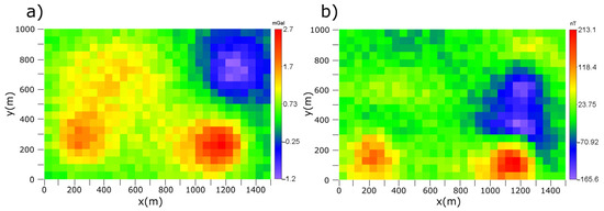
Figure 8.
(a) Gravity anomaly (mGal) and (b) magnetic anomaly (nT) produced by test model 2 in Figure 7. The data were contaminated with Gaussian noise of 5% of the standard deviation in order to test the noise sensitivity of the inversion solutions.
Standard Separate versus Robust Joint Inversion Results of Test Data 2
For this inversion test, maps generated by forward modeling of test model 2 were used as input data automatically generating a domain of 32 × 22 × 15 (10,560) voxels of 50 m on each side. Moreover, 20 iterations were run, and the stopping condition was convergence between models less than 1%. Only a smoothness regularizer was used in standard separate inversion (Equation (17)), while for robust joint inversion (Equation (2)), more information was given to demonstrate how more information apart from a priori data can be crucial to obtain better results. The parameters used in the inversion are described in Table 3.
Table 3.
Inversion parameters for separate and joint inversion.
The results of the experiment at epochs 1, 10, and 20 are plotted in Figure 9 with a general color scale ranging from −1 to 1 g/cm3 and A/m for the gravimetric and magnetic case, respectively. Figure 10 also plots the model convergence of each iteration in percentage, which represents how much a model changes with respect to the past iteration and the RMS error of normalized residuals that reflects the mismatch between the input synthetic data and the data calculated from the inversion models of each iteration.
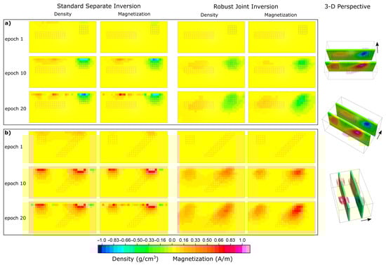
Figure 9.
Profile comparation of separate vs. joint inversion results of test data 2. Density distribution models (g/cm3) and Magnetization distribution (A/m) sliced at (a) 300 m in y-axis and (b) 750 m in y-axis to better show position of four buried bodies. Rose and blue markers represent the original position of buried bodies.
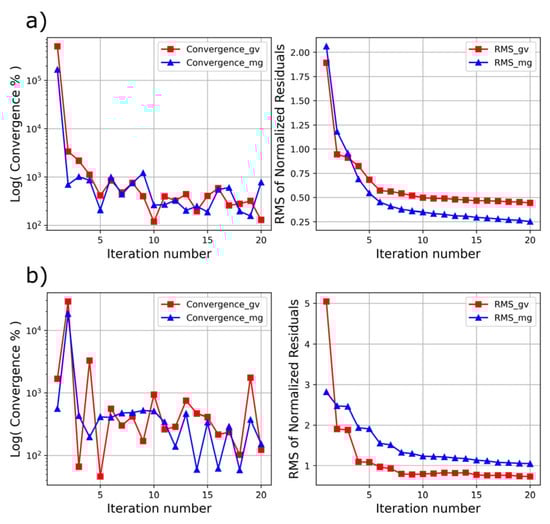
Figure 10.
Model convergence (Equation (18)) and data misfit (Equation (19)) achieved in inversion of test data 2 at each iteration, (a) for standard separate inversion and (b) for our robust joint inversion.
3.3. Field Data Testing
To test the program and the robust joint inversion algorithm, we performed the inversion of preliminary field data from Los Contreras phreatomagmatic maar (Figure 11), located at the San Luis Potosí volcanic field, Central Mexico [84,85]. Gravity data were obtained at 50 m through walks using a CG-5 Autograv gravity meter with a reading resolution of 0.001 mGal. Measurement of the Earth’s magnetic field was realized at the same spots using a GSM-19 high-sensitivity Overhauser effect magnetometer with 0.01 nT resolution and 0.2 nT absolute accuracy. The magnetic field in the area is characterized by B = 41,922.8, I = 50.86, and D = 4.51.
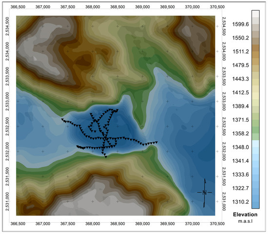
Figure 11.
Topography of the maar Los Contreras, SLP. Acquired gravity and magnetic data location in black marks.
After corrections were performed to the raw data, the residual gravity anomaly was calculated by subtraction of the regional components from the observed complete Bouguer anomaly, and simultaneously, the regional magnetic field was subtracted from the observed magnetic anomaly data. After data reduction, we statistically interpolate the data using variograms to obtain better coverage of the study area and resample a regular mesh at 100 m of spacing, obtaining 128 data points for each (gravity and magnetic) method (Figure 12).
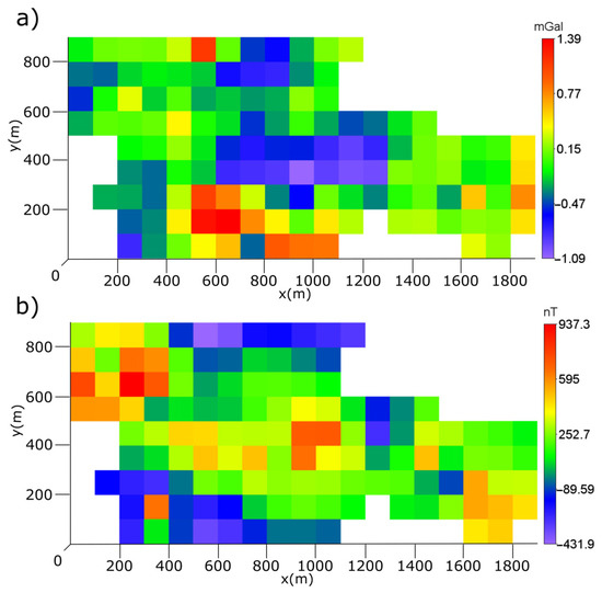
Figure 12.
Observed geophysical data in Los Contreras area. (a) Residual complete Bouguer gravity anomaly and (b) Residual magnetic anomaly.
We performed a joint inversion with a smoothness regularizer for 20 iterations with a stopping condition of convergence between models less than 1%. No a priori information, structural direction, variable standard deviation to data or models was introduced due to better results according to the area geological-structural context, which are beyond the scope of this article. A domain of 21 × 11 × 10 (2310) voxels was automatically generated based on the spatial limits of the input data and the voxel size of 100 m per side. Results are shown in Figure 13, slicing density and magnetization domains from top to bottom at 300 m until no more physical property contrast is visible. Additionally, the convergence and RMS graphs are also displayed in Figure 13.
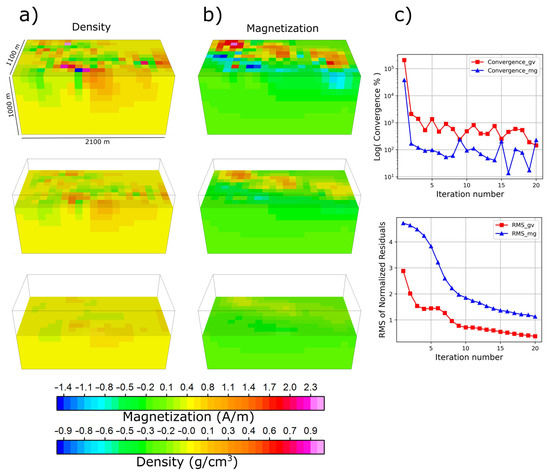
Figure 13.
Inversion results of preliminary field data, slicing the 3-D view each 300 meters from top to bottom until no more physical property contrast is visible, (a) Density contrast, (b) Magnetization contrast and (c) Convergence and RMS plots.
4. Discussion
Here we list the main discussion issues related to the solution to the problem posed in the paper. In brief, they can be summarized as follows:
It is possible to further optimize the computational implementation, e.g., by CPU parallelization using MPI; however, this only decreases the processing time (objective already met) without enhancing memory management. On the other hand, by incorporating variable resolution both horizontally and vertically through cells of varying dimensions, we would be able to differentiate the domain more efficiently, thereby reducing memory usage.
At this point in development, the program is only capable of working with an equal amount of data for both types of input data; likewise, the resolution of the joint inversion models is the same for both geophysical techniques, limiting its application to the spatial coverage of both data types. Additionally, the way we construct our 3D domain does not consider topography yet.
The shown processing times are representative, as they depend on the quantity of data to be processed, how the calculations were implemented, the compiler and the packages used, as well as the capabilities of the hardware employed. Thus, processing times may vary as any of these factors change.
The main advantages of this implementation are (1) the approach to obtain inversion solutions (parametric functional) is versatile, applicable to a wide variety of study objects because the linear regularizers that it integrates seek to promote general characteristics in the solutions, (2) the structural similarity regularizer allows reducing the uncertainty of the results, integrating two geophysical methods within the process of obtaining the solution, overcoming one of the great disadvantages of any geophysical method (ambiguity), finally (3) saves computational costs by reducing processing times which improves the efficiency of the process to obtain results and makes better use of available memory allowing to solve joint inversion problems for larger domains with less powerful hardware.
The use of other linear regularizers, such as the case of L, M, and N, can be incorporated without altering the performance too much since they are part of the expression (Equation (8)), which is calculated only once at the beginning of the inversion process. Therefore, changing the behavior of the solutions with other linear regularizers has no repercussions on the overall performance.
On the other hand, as can be seen in the convergence graphs (Figure 6, Figure 10, and Figure 13), the iterative process is unstable; that is, the models change with respect to the previous iteration by a high percentage. We associate this characteristic to the method we employ to minimize the parametric functional but overall to the use of many regularizers within the minimization process, as we noticed solutions with fewer regularizers active tend to be more stable, however, as also shown in the same figures, there is a tendency to stabilize the solution as the number of iterations increases, while in the RMS graph, it can be seen that the fit of the solutions is very good since early iterations. Therefore, this instability is not a problem for the quality of the results.
Finding the optimal combination of regularization parameter values where a solution exists and a low misfit of solutions with respect to observed data is achieved is a task that becomes more complex as more regularizers are non-zero in the parametric function. It is possible to resort to several methods, such as L-curve plots, which allow the moment of change between under-regularization and over-regularization to be visualized for many trials. The value of each regularization parameter controls the trade-off between fidelity to the observed data and the regularization conditions; in addition, other factors such as initial models, the quantity of a priori information, or data noise levels impact the inversion outcomes, making each particular case different. In this case, we overcame this drawback by using the trial-and-error approach, using near-zero values for regularization parameters and slowly increasing them until we achieved acceptable levels of error. Hence, several trials were performed to obtain these results (Figure 5 and Figure 9). This is an opportunity area to improve by finding a way to obtain good results semi-automatically.
5. Conclusions
The inversion results with structural similarity and greater structural direction constraints (Equation (2)) are an improvement with respect to standard separate inversion (Equation (17)), allowing to better estimate of the form and depth of the buried dike (Figure 5). Despite being sensitive to the noise of the input data, they do present structural similarity, in this example, we give prior information in one method through the cuttings of a pair of hypothetical wells (density in two wells) to show how structural similarity regularizer can use this information together with dip and strike to improve magnetization distribution, while both models can justify observed data. In addition to that, our parametric function proved to better estimate the form and depth of different buried bodies (Figure 9) compared to standard separate inversion.
Processing time does not depend on the size (dimensions) of the cells but on the size of the matrices needed for processing; the major issue in obtaining higher resolution inversion models is the amount of RAM or VRAM to which one has access, as the amount of memory required for an inversion grows exponentially and is highly dependent on the number of voxels in the 3D domain of the models and, to a lesser extent, on the number of observed data. However, good results can be obtained even with lower resolution models (fewer cells), as the minimum resolution required for studies is defined by the scale of the study, the objectives, and the scope of each study.
Having three versions of code allows us to obtain preliminary results within minutes, either by employing the fully parallel or hybrid version of the code, to minimize the total processing time. In cases where the VRAM available on the graphics card falls short, reducing the resolution of the 3D domains during the initial modeling stages proves to be a viable strategy. Once the regularization parameters achieve fidelity to observed data and results align with geologically expected distributions, it is possible to revert to a higher model resolution and utilize the single-core version of the code with associated time-related costs. This is feasible due to the lower cost and ease of obtaining additional RAM instead of VRAM.
Through the analysis of performance and computational costs of serial, parallel, and hybrid implementations, we conclude that as the inversion domain expands, the processing speed could increase from 4× up to 100× times faster, as shown in Table 1, rendering it particularly advantageous for application in larger domains.
Supplementary Materials
The following supporting information can be downloaded at: https://github.com/abdrg/Gram_Joint_Inversion.git accessed on 15 August 2023. In this link the repository of the Fortran code and the test data to reproduce synthetic test model 1 can be found under a BSD license to use the source code in non-free software.
Author Contributions
Conceptualization, methodology, A.D.R.G. and V.Y.; software, data curation, A.D.R.G. validation, V.Y.; investigation, V.Y. and A.D.R.G.; writing—original draft preparation, A.D.R.G. and V.Y.; writing—review and editing, V.Y.; discussion, interpretation of physical results and conclusions, all authors; visualization (preparation of figures), A.D.R.G.; supervision, V.Y.; project administration, V.Y. All authors have read and agreed to the published version of the manuscript.
Funding
This work was supported by CONACYT-Fondos Sectoriales Project A1-S-29604 to Vsevolod Yutsis. Abraham Del Razo received support from CONACYT PhD scholarship with CVU 816921. The APC was partially funded by the Instituto Potosino de Investigación Científica y Tecnológica, A.C.
Institutional Review Board Statement
Not applicable.
Informed Consent Statement
Not applicable.
Data Availability Statement
No applicable.
Acknowledgments
This work was partially supported by CONACYT Project A1-S-29604. Abraham del Razo gratefully acknowledges support from CONACYT Ph.D. scholarship with CVU 816921. The APC was partially funded by the Instituto Potosino de Investigación Científica y Tecnológica, A.C. The authors are grateful to Emilia Fregoso Becerra and Daniel Ignacio Salgado Blanco for their valuable suggestions, which greatly improved the work. The authors are grateful to Graham Matthew Tippett for editing the English version of manuscript.
Conflicts of Interest
The authors declare no conflict of interest.
Appendix A. Linear Operators for Gravimetric and Magnetic Direct Modeling
The operators and are calculated using analytical solutions for straight prisms with the dimensions described by the limits following the development of [77,78] for gravimetry and magnetometry, respectively.
For the number of data and the number of prisms the matrices are defined by:
where:
And are directional cosines of the magnetic field.
Appendix B. Development of the 1st Variation of the Objective Function
We express the parametric functional using the following notation, where ⟨,⟩ denotes an inner product:
The least squares method is used to find the solution, so the first variation of the functional must be calculated and equaled to zero. Using Calculus of Variations, the Gateaux derivative is calculated, whereas most of the terms are quadratic it is trivial:
The variation where is called the Fréchet derivative of A. However, the Fréchet derivative of a linear operator is the operator itself . Additionally, expressing the first variation of the coupling term in inner product form:
The constants are factored using the linearity property of the inner product and adjoint operators are used to obtain the expression:
From the above expression we obtain the Euler equation whose main characteristic is that it expresses the minimum of the parametric functional , i.e., the parameters m with which the parametric functional finds a minimum are a solution to the Euler equation.
Adjoint operators such as simplify to transposes . Since they belong to the reals they have no imaginary part:
The terms can also be regrouped in the following way, which will be useful later:
Appendix C. First Variation of the Structural Coupling Term of the Parametric Functional
The structural coupling term for iteration is expressed as:
For reasons of simplifying the notation a little, is replaced by . For the first variation of the coupling term in the functional with respect to
By applying the linearity property to each term of the matrix, we obtain:
The term is actually the Gramian G of the original functional, but since it does not contain it will be a null term when deriving. Therefore, the variation of the Gramian is expressed as:
By performing the derivative of Gateaux for each term and making use of a property of the inner producer product, we obtain:
For the first term, using the product of inner products :
Deriving with respect to t, then evaluating at the remaining terms:
By using the same procedure to calculate the variations of the other 3 terms, we obtain:
Summing the above 4 terms, the first variation of the Gramian is as follows:
Rearranging and factorizing:
Thus:
where we define as
Similarly, the first variation of the coupling term in the functional with respect to can be obtained:
where:
Finally, the vectors are concatenated to use this new vector in the process of defining the optimal value of .
References
- Wiederhold, H.; Kallesøe, A.J.; Kirsch, R.; Mecking, R.; Pechnig, R.; Skowronek, F. Geophysical methods help to assess potential groundwater extraction sites. Grund.-Z. Der Fachsekt. Hydrogeol. 2021, 26, 367–378. [Google Scholar] [CrossRef]
- Xu, M.L.; Yang, C.B.; Wu, Y.G.; Chen, J.Y.; Huan, H.F. Edge detection in the potential field using the correlation coefficients of multidirectional standard deviations. Appl. Geophys. 2015, 12, 23–34. [Google Scholar] [CrossRef]
- Mauriello, P.; Patella, D. Localization of magnetic sources underground by a probability tomography approach. Prog. Electromagn. Res. 2008, 3, 27–56. [Google Scholar] [CrossRef]
- Blakely, R.J. Potential Theory in Gravity and Magnetic Applications; Cambridge University Press: Cambridge, UK, 1996. [Google Scholar]
- Telford, W.M.; Geldart, L.P.; Sheriff, R.E. Applied Geophysics, 2nd ed.; Cambridge University Press: Cambridge, UK; New York, NY, USA; Port Chester, NY, USA; Melbourne, Australia; Sydney, Australia, 1991; 770p, ISBN 0-521-3269-3-1/0-521-33938-3. [Google Scholar]
- Kearey, P.; Brooks, M.; Hill, I. An Introduction to Geophysical Exploration; John Wiley & Sons: Hoboken, NJ, USA, 2002; Volume 4. [Google Scholar]
- Lowrie, W.; Fichtner, A. Fundamentals of Geophysics; Cambridge University Press: Cambridge, UK, 2020. [Google Scholar]
- Jackson, D.D. The use of a priori data to resolve non-uniqueness in linear inversion. Geophys. J. Int. 1979, 57, 137–157. [Google Scholar] [CrossRef]
- Grana, A.; Passos de Figueiredo, L.; Azevedo, L. Uncertainty quantification in Bayesian inverse problems with model and data dimension reduction. Geophysics 2019, 84, M15–M24. [Google Scholar] [CrossRef]
- Zhdanov, M.S.; Ellis, R.; Mukherjee, S. Three-dimensional regularized focusing inversion of gravity gradient tensor component data. Geophysics 2004, 69, 925–937. [Google Scholar] [CrossRef]
- Pallero, J.L.G.; Fernández-Martínez, J.L.; Bonvalot, S.; Fudym, O. Gravity inversion and uncertainty assessment of basement relief via Particle Swarm Optimization. J. Appl. Geophys. 2015, 116, 180–191. [Google Scholar] [CrossRef]
- Abubakar, A.; Gao, G.; Habashy, T.M.; Liu, J. Joint inversion approaches for geophysical electromagnetic and elastic full-waveform data. Inverse Prob. 2012, 28, 055016. [Google Scholar] [CrossRef]
- Gao, G.; Abubakar, A.; Habashy, T.M. Joint petrophysical inversion of electromagnetic and full-waveform seismic data. Geophysics 2012, 77, WA3–WA18. [Google Scholar] [CrossRef]
- Habashy, T.M.; Abubakar, A. A general framework for constraint minimization for the inversion of electromagnetic measurements. Prog. Electromagn. Res. Symp. 2004, 46, 265–312. [Google Scholar] [CrossRef]
- Spichak, V. Modern Methods for Joint Analysis and Inversion of Geophysical Data. Russ. Geol. Geophys. 2020, 61, 341–357. [Google Scholar] [CrossRef]
- Lelièvre, P.G.; Farquharson, C.G.; Hurich, C.A. Joint inversion of seismic travel times and gravity data on unstructured grids with application to mineral exploration. Geophysics 2012, 77, K1–K15. [Google Scholar] [CrossRef]
- Franz, G.; Moorkamp, M.; Jegen, M.; Berndt, C.; Rabbel, W. Comparison of Different Coupling Methods for Joint Inversion of Geophysical Data: A Case Study for the Namibian Continental Margin. J. Geophys. Res. Solid Earth 2021, 126, e2021JB022092. [Google Scholar] [CrossRef]
- Gallardo, L.A.; Meju, M.A. Joint two-dimensional cross-gradient imaging of magnetotelluric and seismic traveltime data for structural and lithological classification. Geophys. J. Int. 2007, 169, 261–1272. [Google Scholar] [CrossRef]
- Dell‘Aversana, P. Integration of seismic, MT and gravity data in a thrust belt interpretation. First Break 2001, 6, 335–341. [Google Scholar]
- Dell’Aversana, P.; Bernasconi, G.; Miotti, F.; Rovetta, D. Joint inversion of rock properties from sonic, resistivity and density welllog measurements. Geophys. Prosp. 2011, 59, 1144–1154. [Google Scholar] [CrossRef]
- Reimann, C.; Filzmoser, P.; Garrett, R.; Dutter, R. Statistical Data Analysis Explained; John Wiley & Sons: London, UK, 2008. [Google Scholar]
- Kaufman, L.; Rousseeuw, P.J. Finding Groups in Data; John Wiley & Sons: London, UK, 2005. [Google Scholar]
- Williams, C.K.I.; Rasmussen, C.E. Gaussian Processes for Machine Learning; MIT Press: Cambridge, MA, USA, 2006; Volume 2, Number 3. [Google Scholar]
- Kanungo, T.; Mount, D.M.; Netanyahu, N.S.; Piatko, C.D.; Silverman, R.; Wu, A.Y. An efficient k-means clustering algorithm: Analysis and implementation. IEEE Trans. Pattern Anal. Mach. Intell. 2002, 24, 881–892. [Google Scholar] [CrossRef]
- Huberty, C.J. Applied Discriminant Analysis; John Wiley & Sons, Inc.: New York, NY, USA, 1994. [Google Scholar]
- Scales, J.A.; Snieder, R. The anatomy of inverse problems. Geophysics 2000, 65, 1708–1710. [Google Scholar] [CrossRef]
- Fernández-Martínez, J.L.; Mukerji, T.; García-Gonzalo, E.; Suman, A. Reservoir characterization and inversion uncertainty via a family of particle swarm optimizers. Geophysics 2012, 77, M1–M16. [Google Scholar] [CrossRef]
- Fernández-Martínez, J.L.; Fernández-Muñiz, Z.; Pallero, J.L.G.; Pedruelo-González, L.M. From Bayes to Tarantola: New insights to understand uncertainty in inverse problems. J. Appl. Geophys. 2013, 98, 62–72. [Google Scholar] [CrossRef]
- Fernández-Martínez, J.L.; Pallero, J.L.G.; Fernández-Muñiz, Z.; Pedruelo-González, L.M. The effect of noise and Tikhonov’s regularization in inverse problems. Part I: The linear case. J. Appl. Geophys. 2014, 108, 176–185. [Google Scholar] [CrossRef]
- Abdelrahman, E.; El-Arby, H.; El-Arby, T.; Essa, K.S. A Least-squares Minimization Approach to Depth Determination from Magnetic Data. Pure Appl. Geophys. 2003, 160, 1259–1271. [Google Scholar] [CrossRef]
- Abdullahi, M.; Singh, U.K.; Roshan, R. Mapping magnetic lineaments and subsurface basement beneath parts of Lower Benue Trough (LBT), Nigeria: Insights from integrating gravity, magnetic and geologic data. J. Earth Syst. Sci. 2019, 128, 17. [Google Scholar] [CrossRef]
- Kumar, C.R.; Kesiezie, N.; Pathak, B.; Maiti, S.; Tivar, R.K. Mapping of basement structure beneath the Kohima Synclinorium, north-east India via Bouguer gravity data modelling. J. Earth Syst. Sci. 2020, 129, 56. [Google Scholar] [CrossRef]
- Alatorre-Zamora, M.A.; Campos-Enriquez, J.O.; Fregoso, E.; Belmonte-Jiménez, S.I.; Chávez-Segura, R.; Gaona-Mota, M. Basement faults deduction at a dumpsite using advanced analysis of gravity and magnetic anomalies. Near Surf. Geophys. 2020, 18, 307–331. [Google Scholar] [CrossRef]
- Jishun, P.; Wang, X.; Zhang, X.; Xu, Z.; Zhao, P.; Tian, X.; Pan, S. 2D multi-scale hybrid optimization method for geophysical inversion and its application. Appl. Geophys. 2009, 6, 337–348. [Google Scholar] [CrossRef]
- Oldenburg, D. Inversion of electromagnetic data: An overview of new techniques. Surv. Geophys. 1990, 11, 231–270. [Google Scholar] [CrossRef]
- Tarantola, A. Inverse Problem Theory and Methods for Parameter Estimation; Society of Industrial and Applied Mathematics (SIAM): Philadelphia, PA, USA, 2005; ISBN 10:0898715725/13:9780898715729. [Google Scholar]
- Aster, R.C.; Borchers, B.; Thurber, C.H. Parameter Estimation and Inverse Problems, 3rd ed.; Elsevier: Amsterdam, The Netherlands, 2019; 392p, ISBN 978-0-12-804651-7. Library of Congress Cataloging-in-Publication Data; Available online: https://gr.xjtu.edu.cn/c/document_library/get_file?folderId=2777518&name=DLFE-136223.pdf (accessed on 15 August 2023).
- Salem, A.; Ravat, D.; Martin, F.M.; Ushijima, R. Linearized least-squares method for interpretation of potential-field data from sources of simple geometry. Geophysics 2004, 69, 783–788. [Google Scholar] [CrossRef]
- Witter, J.B.; Siler, D.L.; Faulds, J.E.; Hinz, N.H. 3D geophysical inversion modeling of gravity data to test the 3D geologic model of the Bradys geothermal area, Nevada, USA. Geotherm. Energy 2016, 4, 14. [Google Scholar] [CrossRef]
- Panzera, F.; Alber, J.; Imperatori, W.; Bergamo, P.; Fah, D. Reconstructing a 3D model from geophysical data for local amplification modelling: The study case of the upper Rhone valley, Switzerland. Soil Dyn. Earthq. Eng. 2022, 155, 107163. [Google Scholar] [CrossRef]
- Gallardo, L.A.; Meju, M.A. Characterization of heterogeneous near-surface materials by joint 2D inversion of dc resistivity and seismic data. Geophys. Res. Lett. 2003, 30, 1–4. [Google Scholar] [CrossRef]
- Liu, S.; Jin, S.; Xuan, S.; Liu, X. Three-dimensional data-space joint inversion of gravity and magnetic data with correlation-analysis constrains. Ann. Geophys. 2022, 65. [Google Scholar] [CrossRef]
- Zhang, R.; Li, T.; Liu, C.; Huang, X.; Jensen, K.; Sommer, M. 3-D Joint Inversion of Gravity and Magnetic Data Using Data-Space and Truncated Gauss–Newton Methods. IEEE Geosci. Remote Sens. Lett. 2022, 19, 8012105. [Google Scholar] [CrossRef]
- Jacoby, W.; Smilde, P.L. Gravity Interpretation. In Fundamentals and Application of Gravity Inversion and Geological Interpretation; Springer: Berlin/Heidelberg, Germany, 2009; ISBN 978-3-540-85328-2/978-3-540-85329-9. [Google Scholar]
- Al-Garni, M.A. Inversion of residual gravity anomalies using neural network. Arab. J. Geosci. 2013, 6, 1509–1516. [Google Scholar] [CrossRef]
- Al-Garni, M.A. Inversion of magnetic anomalies due to isolated thin dike-like sources using artificial neural networks. Arab. J. Geosci. 2017, 10, 337. [Google Scholar] [CrossRef]
- Núñez-Demarco, P.; Bonilla, A.; Sánchez-Bettucci, L.; Prezzi, C. Potential-Field Filters for Gravity and Magnetic Interpretation: A Review. Surv. Geophys. 2023, 44, 603–664. [Google Scholar] [CrossRef]
- Shang, Y.-J.; Yang, C.-G.; Jin, W.-J.; Chen, Y.-W.; Hasan, M.; Wang, Y.; Li, K.; Lin, D.-M.; Zhou, M. Application of Integrated Geophysical Methods for Site Suitability of Research Infrastructures (RIs) in China. Appl. Sci. 2021, 11, 8666. [Google Scholar] [CrossRef]
- Linde, N.; Tryggvason, A.; Peterson, J.E.; Hubbard, S.S. Joint inversion of crosshole radar and seismic traveltimes acquired at the south oyster bacterial transport site. Geophysics 2008, 73, G29–G37. [Google Scholar] [CrossRef][Green Version]
- Fregoso, E.; Gallardo, L.A. Cross-gradients joint 3D inversion with applications to gravity and magnetic data. Geophysics 2009, 74, L31–L42. [Google Scholar] [CrossRef]
- Moorkamp, M.; Heincke, B.; Jegen, M. A framework for 3D joint inversion of MT, gravity and seismic refraction data. Geophys. J. Int. 2011, 184, 477–493. [Google Scholar] [CrossRef]
- Moorkamp, M.; Roberts, A.W.; Jegen, M.; Heincke, B.; Hobbs, R.W. Verification of velocity-resistivity relationships derived from structural joint inversion with borehole data. Geophys. Res. Lett. 2013, 40, 3596–3601. [Google Scholar] [CrossRef]
- Liu, S.; Wan, X.; Jin, S.; Jia, B.; Xuan, S.; Lou, Q.; Qin, B.; Peng, R.; Sun, D. 2023. Fast 3D joint inversion of gravity and magnetic data based on cross gradient constraint. Geod. Geodyn. 2023, 14, 331–346. [Google Scholar] [CrossRef]
- Newman, G.A. A review of high-performance computational strategies for modeling and imaging of electromagnetic induction data. Surv. Geophys. 2014, 35, 85–100. [Google Scholar] [CrossRef]
- Martin, R.; Monteiller, V.; Komatitsch, D.; Perrouty, S.; Jessell, M.; Bonvalot, S.; Lindsay, M. Gravity inversion using wavelet-based compression on parallel hybrid CPU/GPU systems: Application to southwest Ghana. Geophys. J. Int. 2013, 195, 1594–1619. [Google Scholar] [CrossRef]
- Hou, Z.; Huang, D.; Wei, X. Fast inversion of probability tomography with gravity gradiometry data based on hybrid parallel programming. J. Appl. Geophys. 2016, 124, 27–38. [Google Scholar] [CrossRef]
- Rücker, C.; Günther, T.; Wagner, F.M. pyGIMLi: An open-source library for modelling and inversion in geophysics. Comput. Geosci. 2017, 109, 106–123. [Google Scholar] [CrossRef]
- Ravasi, M.; Vasconcelos, I. An open-source framework for the implementation of large-scale integral operators with flexible, modern high-performance computing solutions: Enabling 3D Marchenko imaging by least-squares inversion. Geophysics 2021, 86, WC177–WC194. [Google Scholar] [CrossRef]
- Fu, N.; Tai, H.M. Accelerated Geophysical Inversion for Airborne Transient Electromagnetic Data Using GPU. In Proceedings of the 2023 IEEE International Conference on Industrial Technology (ICIT), Orlando, FL, USA, 4–6 April 2023; IEEE: Piscataway, NJ, USA, 2023; pp. 1–5. [Google Scholar] [CrossRef]
- Epov, M.I.; Nechaev, O.V.; Glinskikh, V.N.; Danilovskiy, K.N. Pulsed Electromagnetic Sounding of the Bazhenov Formation: High-Performance Computing to Justify a New Geophysical Technology. Russ. Geol. Geophys. 2023, 64, 102–108. [Google Scholar] [CrossRef]
- Zhou, S.; Jia, H.; Lin, T.; Zeng, Z.; Yu, P.; Jiao, J. An Accelerated Algorithm for 3D Inversion of Gravity Data Based on Improved Conjugate Gradient Method. Appl. Sci. 2023, 13, 10265. [Google Scholar] [CrossRef]
- Laloy, E.; Linde, N.; Ruffino, C.; Hérault, R.; Gasso, G.; Jacques, D. Gradient-based deterministic inversion of geophysical data with generative adversarial networks: Is it feasible? Comput. Geosci. 2019, 133, 104333. [Google Scholar] [CrossRef]
- Isaev, I.; Obornev, I.; Obornev, E.; Rodionov, E.; Shimelevich, M.; Dolenko, S. Integration of Geophysical Methods for Solving Inverse Problems of Exploration Geophysics Using Artificial Neural Networks. In Problems of Geocosmos; Springer Proceedings in Earth and Environmental Sciences; Springer: Cham, Switzerland, 2020. [Google Scholar] [CrossRef]
- Liu, M.; Vashisth, D.; Grana, D.; Mukerji, T. Joint Inversion of Geophysical Data for Geologic Carbon Sequestration Monitoring: A Differentiable Physics-Informed Neural Network Model. J. Geophys. Res. Solid Earth 2023, 128, e2022JB025372. [Google Scholar] [CrossRef]
- Wu, X.; Ma, J.; Si, X.; Bi, Z.; Yang, J.; Gao, H.; Zhang, J. Sensing prior constraints in deep neural networks for solving exploration geophysical problems. Proc. Natl. Acad. Sci. USA 2023, 120, e2219573120. [Google Scholar] [CrossRef] [PubMed]
- Dukalski, M.; Rovetta, D.; van der Linde, S.; Möller, M.; Neumann, N.; Phillipson, F. Quantum computer-assisted global optimization in geophysics illustrated with stack-power maximization for refraction residual statics estimation. Geophysics 2023, 88, V75–V91. [Google Scholar] [CrossRef]
- Benning, M.; Burger, M. Modern Regularization Methods for Inverse Problems. arXiv 2017, arXiv:1801.09922. [Google Scholar] [CrossRef]
- Hansen, P.C. Regularization tools: A Matlab package for analysis and solution of discrete ill-posed problems. Numer. Algorithms 1994, 6, 1–35. [Google Scholar] [CrossRef]
- Vozoff, K.; Jupp, D.L.B. Joint Inversion of Geophysical Data. Geophys. J. R. Astron. Soc. 1975, 42, 977–991. [Google Scholar] [CrossRef]
- Zhang, J.; Morgan, F.D. Joint Seismic and Electrical Tomography. In Proceedings of the Symposium on the Applicatión of Geophysical to Engineering and Environmental Problems SAGEEP, Houston, TX, USA, 23–26 March 1997; pp. 391–396. [Google Scholar] [CrossRef]
- Haber, E.; Oldenburg, D. Joint inversion: A structural approach. Inverse Probl. 1997, 13, 63–77. [Google Scholar] [CrossRef]
- Gallardo, L.A. Multiple cross-gradient joint inversion for geospectral imaging. Geophys. Res. Lett. 2007, 34, 1–5. [Google Scholar] [CrossRef]
- Zhdanov, M.S.; Gribenko, A.; Wilson, G. Generalized joint inversion of multimodal geophysical data using Gramian constraints. Geophys. Res. Lett. 2012, 39, 1–7. [Google Scholar] [CrossRef]
- Gallardo, L.A.; Fontes, S.L.; Meju, M.A.; Buonora, M.P.; de Lugao, P.P. Robust geophysical integration through structure-coupled joint inversion and multispectral fusion of seismic reflection, magnetotelluric, magnetic, and gravity images: Example from Santos Basin, offshore Brazil. Geophysics 2012, 77, B237–B251. [Google Scholar] [CrossRef]
- Zhdanov, M.S. Inverse Theory and Applications in Geophysics, 2nd ed.; Elsevier: Amsterdam, The Netherlands, 2015. [Google Scholar] [CrossRef]
- Tu, X.; Zhdanov, M.S. Joint Gramian inversion of geophysical data with different resolution capabilities: Case study in Yellowstone. Geophys. J. Int. 2021, 226, 1058–1085. [Google Scholar] [CrossRef]
- Banerjee, B.; Das Gupta, S.P. Gravitational Attraction of a Rectangular Parallelepiped. Geophysics 1977, 42, 1053–1055. [Google Scholar] [CrossRef]
- Bhattacharya, B.K. Magnetic Anomalies Due to Prism Shaped Bodies with Arbitrary Polarization. Geophysics 1964, 29, 517–531. [Google Scholar] [CrossRef]
- Reid, J. The new features of Fortran 2008. ACM SIGPLAN Fortran Forum 2008, 27, 8–21. [Google Scholar] [CrossRef]
- Gallardo, L.A.; Meju, M.A. Joint two-dimensional DC resistivity and seismic travel time inversion with cross-gradients constraints. J. Geophys. Res. 2004, 109. [Google Scholar] [CrossRef]
- Li, Y.; Oldenburg, D.W. 3-D inversion of magnetic data. Geophysics 1996, 61, 394–408. [Google Scholar] [CrossRef]
- Li, Y.; Oldenburg, D.W. 3-D inversion of gravity data. Geophysics 1998, 63, 109–119. [Google Scholar] [CrossRef]
- Varfinezhad, R.; Parnow, S.; Florio, G.; Fedi, M.; Mohammadi Vizheh, M. DC resistivity inversion constrained by magnetic method through sequential inversion. Acta Geophys. 2023, 71, 247–260. [Google Scholar] [CrossRef]
- Aranda-Gómez, J.J.; Luhr, J.F.; Housh, T.B.; Valdez-Moreno, G.; Chávez-Cabello, G. El volcanismo tipo intraplaca del Cenozoico tardío en el centro y norte de México: Una revisión. Bol. Soc. Geol. Mex. 2005, 57, 187–225. [Google Scholar] [CrossRef]
- Peredo, C.R.; Yutsis, V.; Martin, A.J.; Aranda-Gómez, J.J. Crustal structure and Curie point depth in Central Mexico deduced from the spectral analysis and forward modeling of potential field data. J. S. Am. Earth Sci. 2021, 112, 103565. [Google Scholar] [CrossRef]
Disclaimer/Publisher’s Note: The statements, opinions and data contained in all publications are solely those of the individual author(s) and contributor(s) and not of MDPI and/or the editor(s). MDPI and/or the editor(s) disclaim responsibility for any injury to people or property resulting from any ideas, methods, instructions or products referred to in the content. |
© 2023 by the authors. Licensee MDPI, Basel, Switzerland. This article is an open access article distributed under the terms and conditions of the Creative Commons Attribution (CC BY) license (https://creativecommons.org/licenses/by/4.0/).