Abstract
The generalized k- formulation provides a relatively new flexible eddy-viscosity Reynolds-averaged Navier–Stokes modeling approach to turbulent flow simulation, where free coefficients allow for fine-tuning and optimal adjusting of the turbulence closure procedure. The present study addressed the calibration of this versatile model for the aerodynamic design of an innovative mid-range commercial airplane by carrying out a series of simulations for varying model coefficients. Comparing the different solutions with each other, as well as with reference experimental and higher-fidelity numerical data, the performance of the generalized procedure in predicting the aerodynamic loading on the aircraft model was systematically examined. While drawing particular attention to the high-lift regime, the set of model parameters giving the best results was practically determined.
1. Introduction
Due to the marked environmental impact of increased air transportation that is expected in the future, the long-term scenarios for civil aviation are mostly concerned with reducing carbon dioxide (CO2) and nitrous oxide (NO) emissions. The release of these substances from aviation is estimated to be more dangerous than comparable emissions at sea level, making it a significant driver of the climate change. In fact, though recent advancement in airframe and engine technologies leads to increased aircraft efficiency and reduced emissions, the total amount of global aviation emissions could nevertheless increase as a result of the predicted large rise in air transport [1]. To understand how potential next-generation aircraft might look, alternative and environmentally friendly energy sources, as well as modern aircraft designs, need to be considered, because it appears that the set-out goals cannot be achieved using traditional airframes and classical propulsion systems [2].
In the context of future aircraft technologies, computational fluid dynamics (CFD) has been continuously developing as a powerful design and analysis tool, where novel and physics-based numerical methods have gained great attention [3]. Distinguishing features for the aircraft design based on CFD methods include geometric flexibility, accuracy and efficiency, robustness, and scalability. Basically, in the aeronautical industry, the low-cost Reynolds-averaged Navier–Stokes (RANS) simulation remains the most widely followed approach for engineering design, analysis, and optimization of high-Reynolds-number flows [4]. The method, which is generally based on the turbulent eddy-viscosity concept, has been proven to be quite useful in determining the mean flow over airplanes at cruising speeds, being actively employed in the design of the most recent commercial aircrafts by leading companies [5].
In the framework of aerodynamic applications, although the Spalart–Allmaras one-equation model [6] remains often used, owing to its low computational complexity, two-equation eddy-viscosity turbulence models have become very popular. Also, considering the unsuitability of the k- model for problems involving adverse pressure gradients, large separations, and reattachments, the k- model is the one usually employed. In particular, the shear stress transport (SST) version of this model likely represents the most commonly used model in the aerospace industry, given its high accuracy-to-cost ratio [7]. Indeed, the k- SST model provides a better prediction of flow separation than most RANS models, owing to its good behavior in adverse pressure gradients. On the negative side, it causes unphysical large turbulence levels in stagnation flow regions, even though this effect is much less pronounced than with the k- model.
However, unfortunately, the RANS-based methods frequently fail to predict highly separated flows, which are dominated by unsteady flow structures with a broad range of scales and, thus, require more complex modeling of the turbulence Reynolds stresses [8]. On the other hand, scale-resolving simulation (SRS) methods, such as large eddy simulation (LES) and hybrid RANS-LES techniques, which are known to be significantly more accurate, are generally deemed to be prohibitively expensive by industrial researchers [9]. In addition, the wide range of flow configurations, depending on either geometry (shape, angle of attack, computational domain) or freestream conditions (Reynolds number, turbulence intensity), makes it difficult to accurately predict practical aeronautical flows using a single turbulence model, amplifying the unavoidable inconsistencies between experiments and numerical simulations [10]. In fact, the development of universal modeling techniques, especially valid for largely separated flows, is critical in achieving the CFD technology needs for modern aircraft design.
To overcome some limitations of the RANS approach, a novel generalized turbulence modeling procedure was recently introduced in the framework of the CFD code Ansys Fluent 2023 R2 [11]. This commercial software package is based on the finite volume (FV) approach, where the conservation principles are applied over each control volume, representing a commonly used tool for building virtual wind tunnels in the aerospace industry [12]. The new procedure is referred to as a generalized k- (GEKO) model, since it constitutes a reformulation of this well-established two-equation eddy-viscosity model. The proposed formulation employs six free coefficients that can be tuned by the user without compromising the built-in model calibration for fundamental flows. As a result, CFD analysts can optimize the turbulence closure procedure for the particular application in a safe parameter space.
Furthermore, with the advancement of machine learning (ML) algorithms, which are able to make predictions based on huge amounts of available flow data, data-driven RANS turbulence modeling has been recently developing [13]. The data extracted from either experiments or high-fidelity CFD simulations are infused into the learning procedure, while ML techniques are used to link the turbulence modeling behavior to geometric and mean flow variables [14]. In the future, the GEKO model could evolve into an adaptive data-driven turbulence modeling procedure, where the primary objective of achieving high prediction capability is pursued by training the free coefficients using available data and artificial intelligence algorithms rather than exploiting the various traditional turbulence models [15].
The very first step toward the development of an innovative data-driven RANS approach supplied with the GEKO scheme will be taken here by assessing the capability of the generalized model to predict aeronautical flows of practical engineering interest, which is the main aim of this work. For this purpose, the computational evaluation of the mean turbulent flow around the scaled model of a modern regional turboprop aircraft is performed. A series of different RANS calculations will be conducted, where the free coefficients fine-tuning methodology will be proven by comparing the various solutions with each other as well as to both wind tunnel (WT) and higher-fidelity numerical data. Drawing particular attention to the stall regime of the cruise wing, it will be demonstrated that two free parameters of the generalized model, namely, the separation and the near wall coefficients, play the main role in adjusting the prediction of the separated boundary layer (BL) flow on the main wing of the aircraft model. This way, the current investigation provides a clear preliminary idea of the effectiveness of the new GEKO concept, paving the way for future further developments for complex full aircraft configurations.
The remainder of this paper is organized as follows. In Section 2, the generalized two-equation turbulence model is briefly presented together with the reference higher-fidelity SRS method. The particular aeronautical application under consideration is described in Section 3, where the main settings of the numerical calculations are also provided. The results of the model calibration are made known and discussed in Section 4, while some concluding remarks are drawn in Section 5.
2. Turbulence Modeling
In the RANS framework, two-equation eddy-viscosity turbulence models have gained great popularity for industrial CFD applications. These models solve two partial differential equations to calculate two independent turbulence variables for determining the turbulent viscosity field. The basic models typically include some coefficients that can be adjusted to fit the particular flow problem, being calibrated to match experimental findings for fundamental flows (flat plate BL, free shear flows, decaying freestream turbulence). However, these coefficients must meet a number of different criteria while being linked with each other. Due to the limited flexibility of the basic models, several different versions have been developed for specific purposes. In particular, since its conception, the k- model has been constantly revised and improved, becoming one of the most commonly used RANS models for highly separated flows [7,16]. For instance, this two-equation model was recently further developed for the wavelet-based adaptive RANS approach [17]. The modeling procedure uses the turbulent kinetic energy k and the specific turbulence dissipation rate as additional turbulence variables. In the current work, the SST version of the k- model was used as the baseline RANS model [7]. The unknown Reynolds stresses are approximated by means of the classical Boussinesq hypothesis:
where is the deviatoric component of the resolved strain-rate tensor. The turbulent eddy-viscosity is determined in terms of the resolved turbulence variables as follows:
where a realizability constraint is imposed.
2.1. Generalized Two-Equation Turbulence Model
The new GEKO procedure has been recently introduced as a two-equation eddy-viscosity turbulence model capable of providing a single RANS approach that may be customized to a wide range of general flow conditions and applications [11]. The model has been claimed to achieve flexibility by extending the k- SST model with six free coefficients that can be prescribed by the user without compromising the fundamental model calibration for both free shear flows and boundary layers. This allows the user to fine-tune the turbulence closure in a safe parameter space, which requires (at least in principle) no advanced skills or great knowledge in turbulence modeling and simulation. Even though not fully described in the literature, this generalized modeling procedure appears very promising, and various works calibrating the GEKO model coefficients for different industrial fluid dynamics applications have been presented, e.g., [18,19,20].
Following the GEKO approach, the transport equations for the two turbulence variables are reformulated as:
where the additional functions , , and contain the free model coefficients that were introduced [11]. In the above equations, represents the production of turbulence kinetic energy. Standard values can be used for the constants , , and as well as for the turbulent Prandtl numbers and [16].
The six free parameters of the GEKO model are summarized in Table 1 together with their specific controlling function, recommended range of variation, and default value [21]. Two of these coefficients are explicitly designed for wall-bounded flows, namely and , while is however correlated with . The coefficient takes into account the corner flow correction. In this study, the effect of these four coefficients was systematically examined for testing the accuracy of the model in predicting aeronautical flows of engineering significance. The other two coefficients, controlling the accurate prediction of jet flows () and flows with curvature (), were not considered here while being maintained to the associate default values.

Table 1.
Specific function and recommended range of variation for the GEKO parameters [21].
2.2. Scale-Resolving Simulation
The present RANS results were validated against the data attained using a more sophisticated SRS method. Specifically, to generate a reference high-fidelity solution, we used the stress-blended eddy simulation (SBES) approach, which represents a hybrid RANS-LES method specially developed for industrial CFD [4]. Basically, SBES follows the same principle as detached-eddy simulation (DES), using RANS for near-wall flows and LES for bulk flows [22], with the turbulent eddy-viscosity being determined through model blending:
The main difference with respect to previous hybrid formulations is that SBES employs a much stronger shielding function by adopting a novel methodology of combining RANS and LES approaches to achieve optimal performance. In practice, SBES exhibits a faster transition between the two different solutions, resulting in lower eddy-viscosity levels and more resolved turbulent fluctuations. This makes it a suitable method for highly separated shear layer flows of aeronautical interest.
The SBES approach provides a certain flexibility to choose different formulations for the RANS and LES components. In this study, the k- SST model [7] was used for RANS in conjunction with the wall-adapting local eddy-viscosity (WALE) model [23] for LES. While the k- SST model is commonly taken as the benchmark for developing data-driven methods in applied computational aerodynamics [24], the WALE approach was selected as a straightforward LES method that automatically provides vanishing turbulent viscosity for laminar shear flows.
Finally, it should be noted that at present, some important details of both the above modeling procedures are still proprietary. For instance, the exact definition of the GEKO functions , , and in (4), as well as that of the SBES function in (5) (containing the complexity of the model), is not publicly available.
3. Aeronautical Application
The aerodynamic analysis of a new mid-range commercial airplane (with an advanced wing design) was used as an example of aeronautical engineering applications [25].
3.1. Engineering Case Study
The aircraft model was taken from the EU-funded project LOSITA (low subsonic investigation of a large complete turboprop aircraft), where the design and testing of an advanced turboprop regional aircraft was tackled. The experimental campaign, with the various WT conditions simulating the cruise, take-off and landing configurations, allowed for an accurate evaluation of the low-speed performance of the associate scaled-down (1:) aircraft model [26].
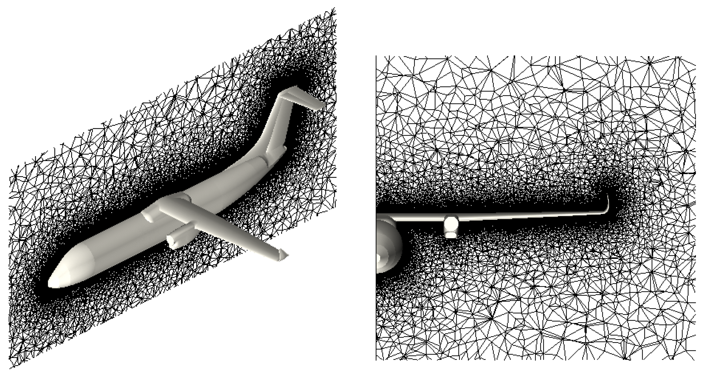
In the present work, three-dimensional CFD computations were conducted to predict the mean turbulent flow around the aircraft model that was provided by the industrial researchers. The simplified aircraft geometry, which is depicted in Figure 1, contained the horizontal and vertical tails as well as the engine nacelle. The model has a length of m, a height of m, and a span of m. The clean configuration of the aircraft was considered, with no high-lift surfaces deployed, while not modelling the effect of the propellers. The calculations were performed for a freestream velocity of 68 m/s, with the Mach and Reynolds numbers corresponding to and , respectively, where the mean aerodynamic chord (MAC) was used as a reference length [26].
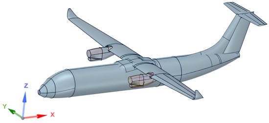
Figure 1.
Computational geometry of the mid-range aircraft model.
The “free-air” simulations (as neither the WT walls nor the model support system were included in the computational geometry) were conducted for zero sideslip angle () while varying the incidence angle in a typical range of interest (that is, ) [26]. Owing to the mean flow symmetry, the computational domain was constructed around the semi-aircraft geometry model with while imposing a symmetry boundary condition at . Specifically, the governing equations were solved in a hemisphere with a radius of 100 MAC. Figure 2 shows a schematic illustration of the computational domain with artificially reduced size. As to the boundary conditions, the aircraft surfaces were considered as adiabatic no-slip walls, while characteristic-based relations were employed for the farfield conditions. Note that some further details can not be provided for industrial property reasons.
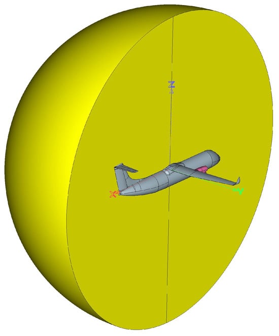
Figure 2.
Schematic illustration of the hemispherical computational domain for (not real scale).
3.2. CFD Solver Settings
In the framework of the FV-based CFD code Ansys Fluent, the compressible RANS governing equations were solved employing the pressure-based coupled flow solver, where the cell face fluxes were determined adopting the Roe scheme. The pressure field was discretized with the central difference scheme. For momentum and turbulence variables, a second-order upwind technique was employed while adopting the least-squares cell-based method for computing the gradients. The resulting large sparse linear system was solved using the AmgX library, which provides a drop-in CPU/GPU acceleration of distributed algebraic multigrid and preconditioned iterative methods. The method allows the parallel solver to minimize communication costs while fully taking advantage of the available high-performance computing (HPC) resources. The interested reader can find more details, for instance, in [27]. Also, the parallel computations were realized by following a domain decomposition approach using the partitioning tool Metis.
As to reference SBES, the corresponding unsteady solution was computed using a second-order implicit iterative dual time-advancement method, starting from the baseline SST RANS solution as initial condition. The constant time-step size was such that the cell-convective Courant number was of the order unity in the vicinity of the aircraft surfaces, while ten inner loop iterations for every time step were used to ensure the convergence of the normalized residuals. The spatial discretization of the convective terms in the momentum equation was performed through bounded central differencing, which enables low numerical diffusion but still ensures stability by blending in first and second-order upwind schemes in case the convection boundedness criterion is violated [28]. The simulation was run for ten convective flow units to achieve statistically steady flow conditions. Then, the time statistics were accumulated for a further ten units, resulting in less than a half drag count fluctuation of the varying mean drag value.
3.3. Mesh Generation
The mesh generation was carried out using the commercial software Pointwise V18.4 R4, by following an iterative grid refinement procedure, as is usual for industrial CFD applications [29]. First, the various surfaces of the aircraft model were meshed using triangular elements. For instance, the tessellation of the main wing suction-side, including the winglet, is depicted in Figure 3, where the mesh resolution is artificially reduced for illustration purposes. Note that the surface grid was refined at the leading and trailing edges of the wing. For the production mesh, fine surface grid cells with a linear size close to MAC were used. Then, three-dimensional viscous-type unstructured meshes were constructed by employing prism layers along the solid walls and tetrahedral cells in the rest of the computational domain. The discretization of the BL regions was performed using the T-Rex meshing algorithm, with the first cell spacing dictated by the desired near-wall resolution. The FV mesh had two prismatic layers with constant cell spacing in the wall-normal direction with a subsequent growth rate that was less than or equal to . For illustration, the slices through the three-dimensional mesh at and are drawn in Figure 4.
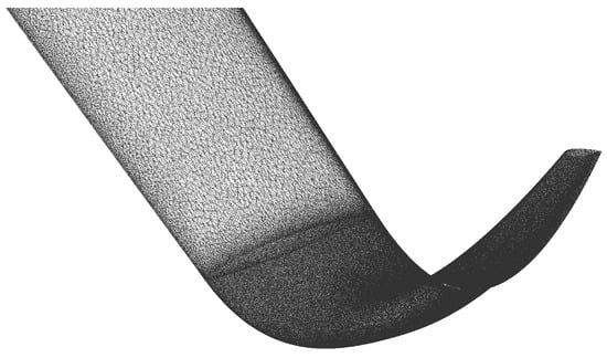
Figure 3.
Surface mesh on the main wing, including the winglet.
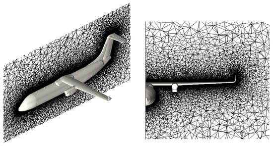
Figure 4.
Slices through the prismatic/tetrahedral three-dimensional mesh at (left) and (right).
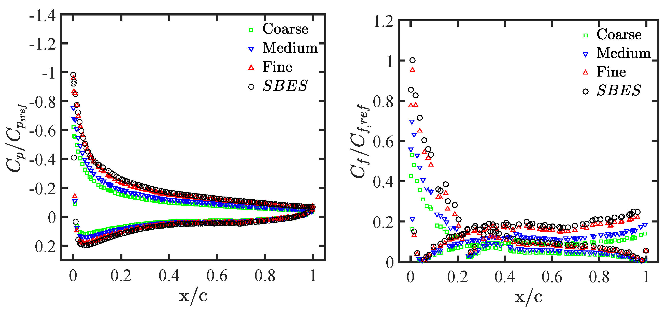
The production mesh used for investigating the GEKO procedure was selected after a preliminary grid convergence analysis, which was performed for the baseline SST RANS. Three different (similar) grids were tested with varying near-wall mesh resolution, corresponding to (coarse), 10 (medium), and 1 (fine), for the first wall spacing. Practically, given the target resolution to be achieved, a tentative simulation was initially carried out by prescribing the first cell size based on the theoretical estimation of the local skin-friction for the flat-plate turbulent BL flow. Then, by measuring the actual value of resulting from the simulation, the first wall spacing was suitably adjusted. Finally, based on this procedure, a sufficiently small first wall distance for the whole mesh was selected.
The convergence of the SST RANS solution toward the high-fidelity SBES, for increasing spatial resolution, is demonstrated by looking at the results obtained for , for example. Figure 5 shows the normalized pressure and skin-friction coefficient distributions for the wing section at the semispan fraction , with b representing the wing span. Moreover, the errors for the predicted aerodynamic force coefficients for the different solutions with varying mesh resolution are reported in Table 2.
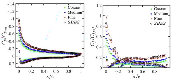
Figure 5.
Normalized sectional pressure (left) and skin-friction (right) coefficients at , for , and varying mesh resolution compared to SBES.
Table 2.
Number of FV cells and errors for the predicted aerodynamic force coefficients at against the experimental data for varying mesh resolution.
4. Results and Discussion
The practical effect of modifying the four GEKO coefficients under consideration, which are , , , and , was systematically examined by carrying out a series of different steady RANS simulations. Specifically, a parametric study, where only one parameter was varied while keeping the others constant, was performed. The different RANS solutions were compared with each other as well as with the reference high-fidelity SRS. This allowed for a clear understanding of the influence of each model coefficient.
4.1. Varying Coefficient
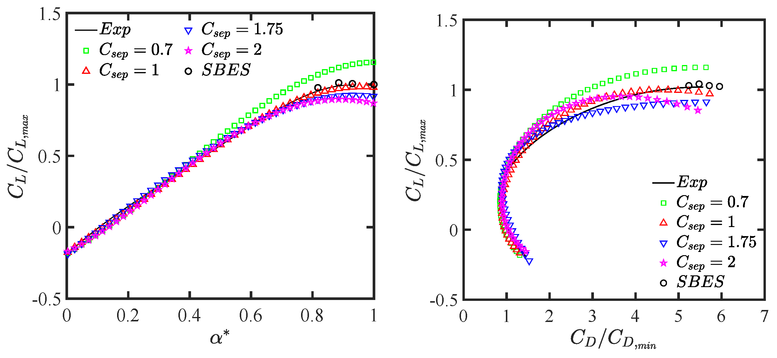
The numerical predictions of the global aerodynamic loading on the aircraft model, for varying coefficients, are reported in Figure 6, in terms of lift curve and drag polar, compared to WT data [26]. Here, the lift and drag coefficients are normalized by the experimental values of and , respectively, while the angle of incidence is normalized as . To perform a systematic analysis, four different calculations were carried out for each incidence by selecting different values for the coefficient in the recommended range, namely , 1, , and 2 (see Table 1). Moreover, a few (costly) SBES solutions were obtained for the stall regime, namely for , demonstrating the conformity between the present SRS results and experimental data.
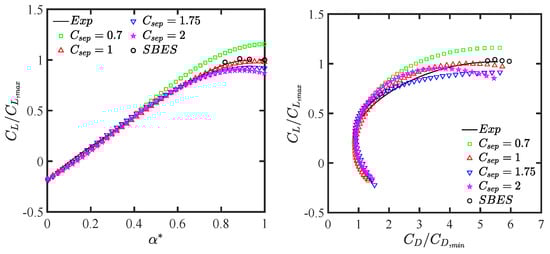
Figure 6.
Global aerodynamic loading on the aircraft model: lift curve (left) and drag polar (right), for different values of , compared to SBES and experimental data.
In the linear lift regime, the predicted lift curve shows good agreement with the experiments regardless of the level, while marked discrepancies are observed at high angles of attack. Apparently, both the lift curve slope and the zero-lift angle result in being quite accurate. The errors against experimental values for these aerodynamic parameters, together with that for the zero-lift drag coefficient , are summarized in Table 3. Furthermore, by inspection of the drag polar, the drag force is evidently overestimated by choosing the default value , especially at high incidences. Note that near the maximum lift condition, the variation of affects both drag and lift forces. As expected, the “separation” coefficient plays a key role for adjusting the predicted aerodynamic performance of the aircraft model. As it will be demonstrated in the following, this strong dependence has to be attributed to the more or less accurate prediction of the separated turbulent flow on the main wing of the aircraft. In fact, the free parameter directly affects the onset and evolution of the separated BL flow on the suction-side of the main wing, which becomes crucial at high incidences. Therefore, we focused our attention on the GEKO prediction of the cruise wing aerodynamics at the stall regime by considering three different angles of attack, namely , , and .
Table 3.
Errors for the predicted aerodynamic parameters, against the experimental data, for different values of .
First, let us note that due to the three-dimensional character of the wing BL, the choice of also influenced the spanwise behavior of the aerodynamic loading. This is clearly illustrated, for instance, by looking at the contours of the skin-friction coefficient on the suction-side of the main wing, which are depicted in Figure 7, for the three different incidences and two different values of .
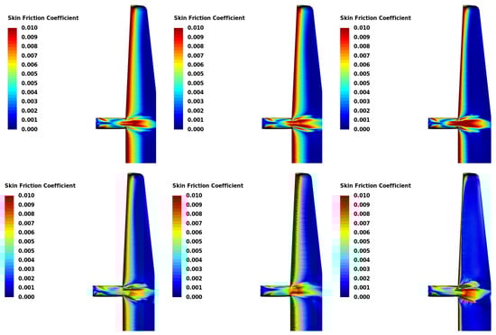
Figure 7.
Contours of surface skin-friction coefficient on the main wing suction-side, for (top) and 2 (bottom), at three different incidences that are (left), (middle), and (right).
Apparently, the choice of the higher value for this parameter, which is , alters the BL flow evolution along the wing, providing the early onset of flow separation. On the contrary, fixing provided skin-friction contours that are practically indistinguishable from the higher-fidelity SBES solution (not reported for brevity).
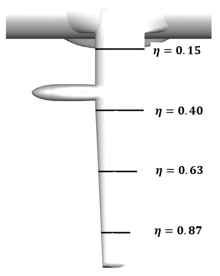
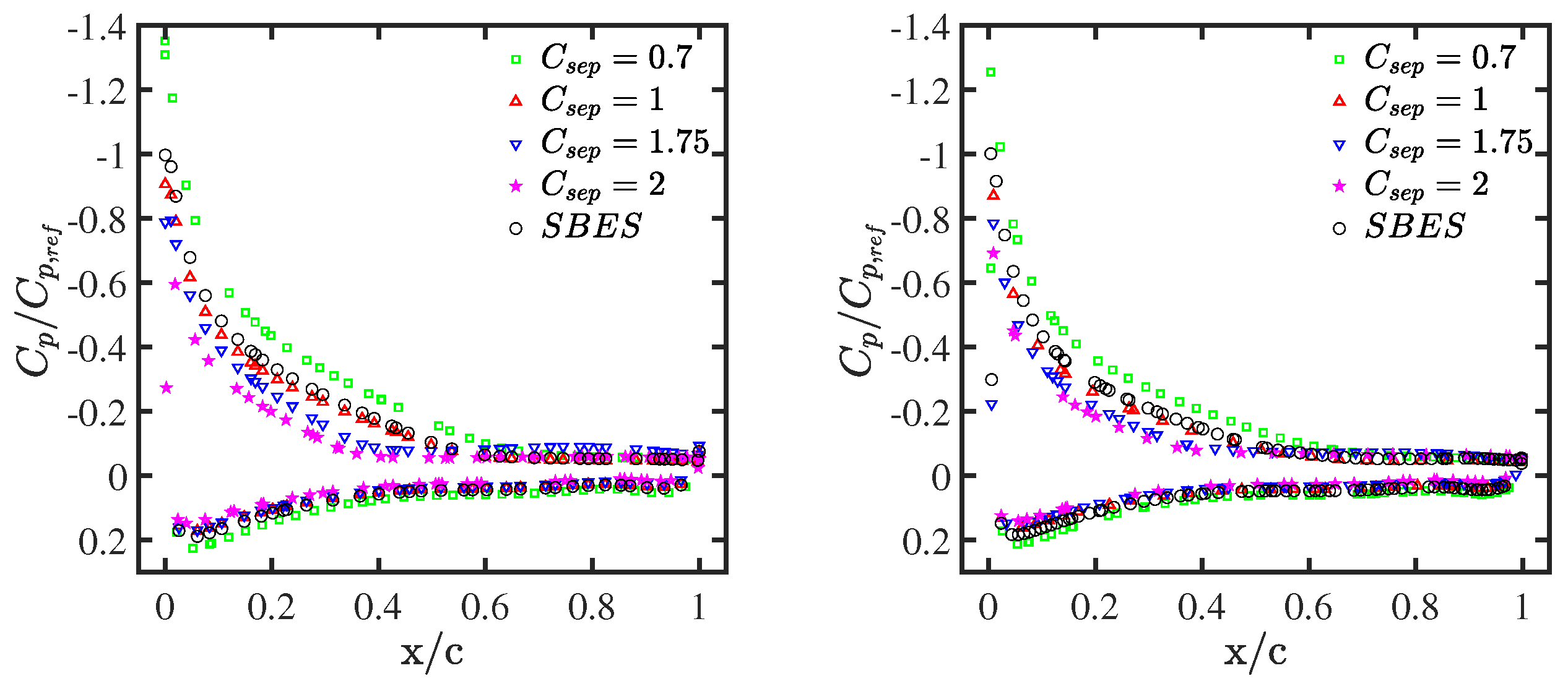
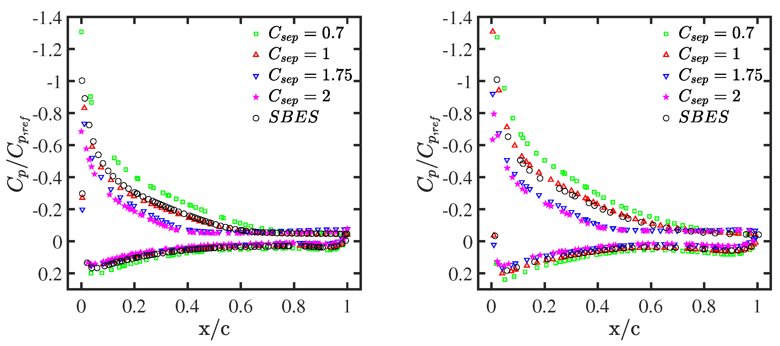
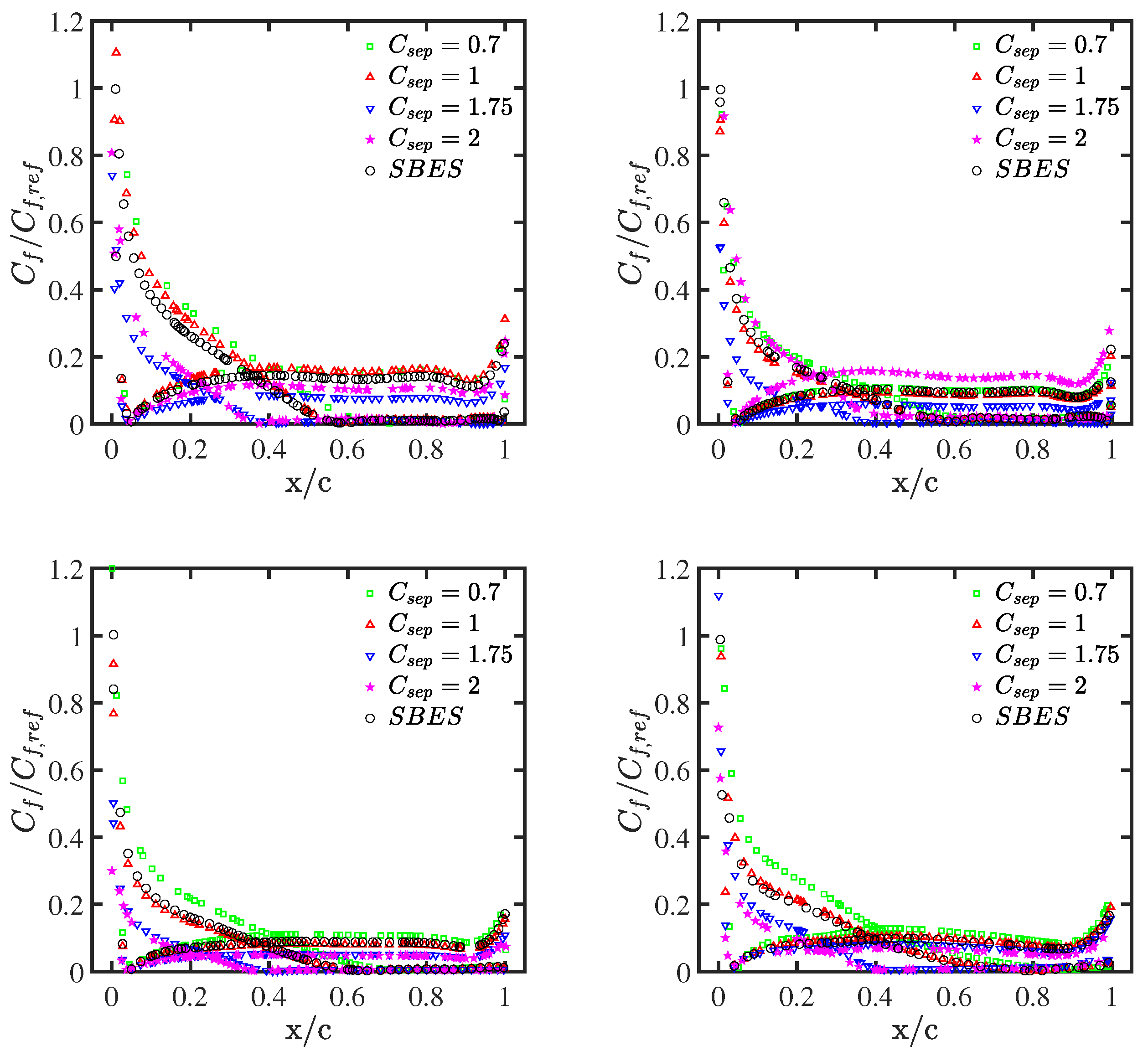
The quantitative analysis of the main wing aerodynamics was performed by examining the distributions of sectional pressure and skin-friction coefficients at four different spanwise locations. As depicted in Figure 8, the selected sections correspond to the semispan fractions: (near the wing root), (near the engine nacelle), , and (near the wing tip). Unless otherwise indicated, the following data refer to the case , while similar results obtained for the other two incidences are not reported for conciseness. Figure 9 shows the pressure coefficient distributions, with the corresponding skin-friction coefficient distributions being drawn in Figure 10, while making a comparison with the time-averaged SBES results. The aerodynamic loading coefficients are normalized by using the following reference data: and .

Figure 8.
Spanwise locations of the four main wing sections under consideration.
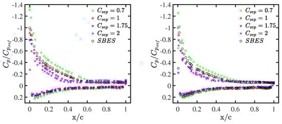
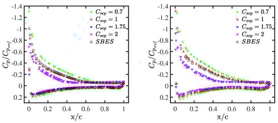
Figure 9.
Normalized sectional pressure coefficient at (top left), (top right), (bottom left), and (bottom right) for different values of compared to SBES.
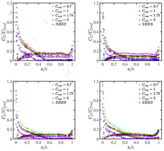
Figure 10.
Normalized sectional skin-friction coefficient at (top left), (top right), (bottom left), and (bottom right) for different values of compared to SBES.
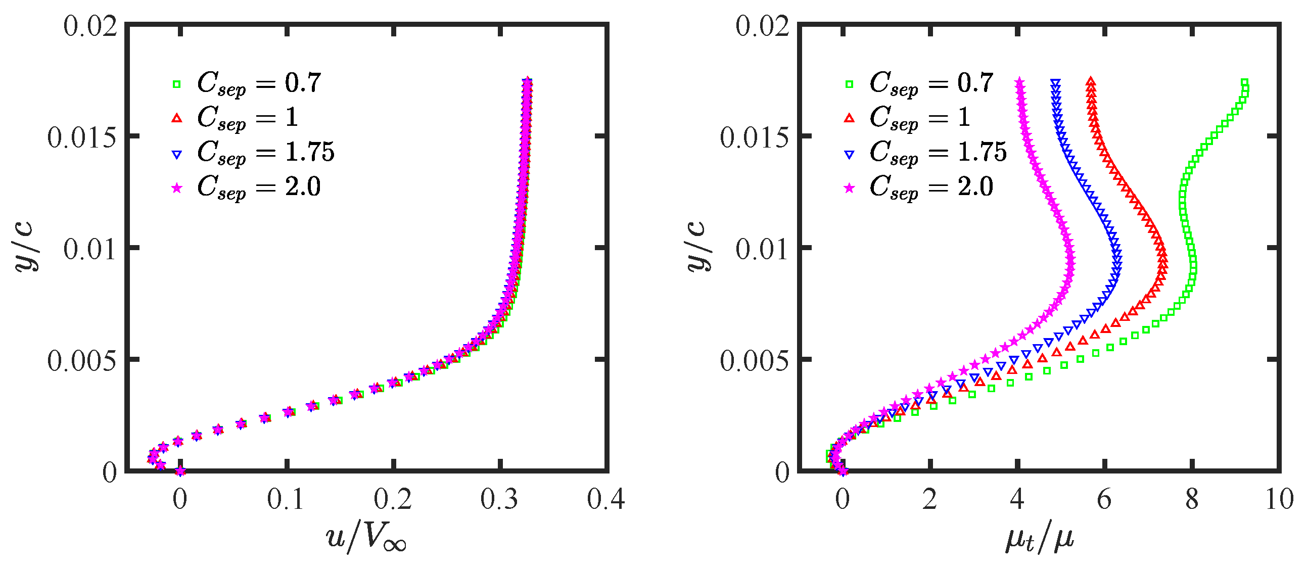
By inspection of these figures, the higher levels of (say ) provide completely wrong or anticipated BL separations. Apparently, decreasing leads to more accurate predictions of pressure recovery regions while approaching the reference SBES solution. This is particularly evident for the wing sections where the BL separation is more important. For instance, Figure 11 shows the velocity profile at and , normalized by the freestream velocity , along with the profile of the turbulent viscosity ratio that is . While the BL velocity field is practically not affected by the variation of , the modeled eddy-viscosity increases with decreasing this parameter, leading to less sensitivity of the BL flows to the high adverse pressure gradients on the suction-side of the wing. Therefore, the separation onset is more correctly represented by the lowest levels of this parameter. However, for , the eddy-viscosity was overly increased, and the accuracy of the solution was lost, with both pressure and skin-friction coefficients being overestimated. On the contrary, by increasing too much this parameter, the BL separation is anticipated, and the separated flow region is erroneously enlarged. This is particularly evident by looking at the skin-friction coefficient plots, where determines the separated flow zone. Overall, the prescription of resulted in being the optimal choice for the present aeronautical application (when keeping the other coefficients unchanged).
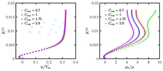
Figure 11.
Normalized profiles of velocity (left) and turbulent viscosity (right) at and .
4.2. Varying Coefficient
Unfortunately, modifying the parameter alters the modeled eddy-viscosity in the entire flow field, including free shear flow regions (such as wakes). In particular, decreasing and, thus, increasing the eddy-viscosity, results in higher spreading rates and turbulence levels. To avoid a possible negative impact on free shear flows, the following optimal value of the “mixing” coefficient was suggested in the original report [21]:
which corresponds to the default choice in Table 1. In practice, the above correlation decreases with decreasing to maintain the correct spreading rate.
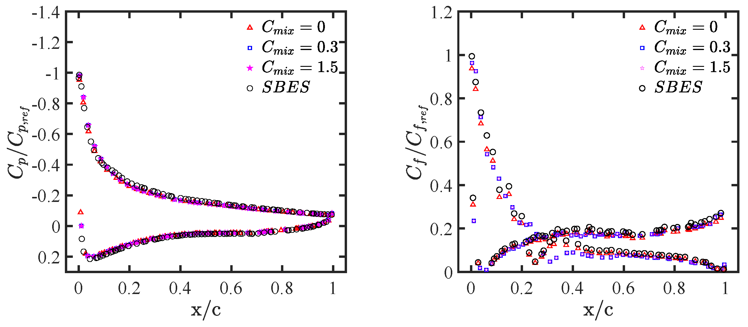
Herein, to empirically test the effect of varying , two additional calculations were performed, fixing by prescribing either or . Figure 12 shows the predicted distributions of sectional pressure and skin-friction coefficients compared to the solution corresponding to the default value that is as well as to SBES. Only the wing section at is reported, as the effect of varying resulted in being practically negligible almost everywhere. The superiority of the suggested default level (6) is however confirmed when looking at the skin-friction distribution.
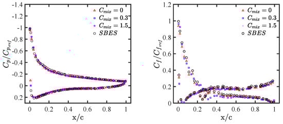
Figure 12.
Normalized sectional pressure (left) and skin-friction (right) coefficients at for different values of compared to SBES.
4.3. Varying Coefficient
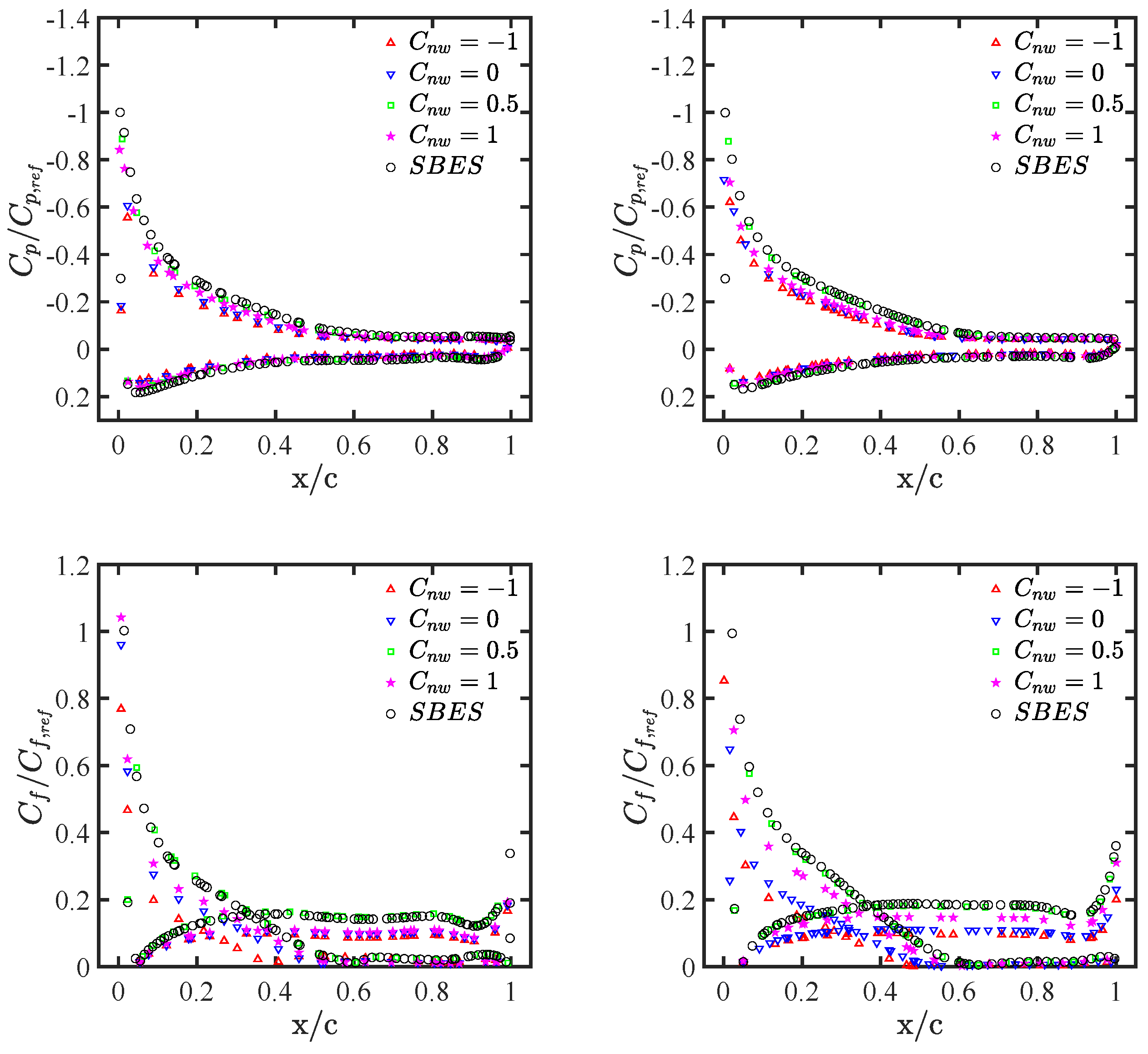
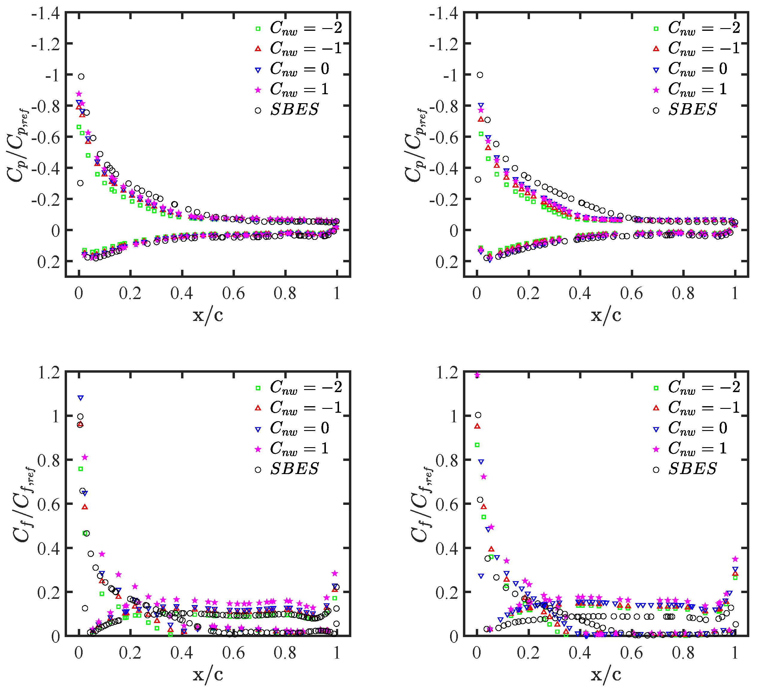
The “near-wall” coefficient is designed to control the inner part of BL flows while not affecting free shear flows [21]. Specifically, both the wall shear-stress and wall heat transfer rate (for non-adiabatic walls) increase as this parameter increases (in non-equilibrium flows). Therefore, the surface skin-friction exhibits a larger sensitivity to this parameter than the surface pressure, as is confirmed by looking at the coefficient distributions reported in Figure 13, corresponding to GEKO solutions with and various levels of . According to these results, fixing the default value that is represents a good choice for this particular application.
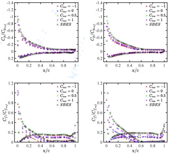
Figure 13.
Normalized sectional pressure (top) and skin-friction (bottom) coefficients at (left) and (right) for and different values of compared to SBES.
However, in order to determine whether the previous conclusion about the optimal choice of was affected by the prescribed coefficient, a further analysis was conducted by setting at the suggested default value—that is, —while varying . By looking at the sectional pressure and skin-friction coefficient distributions drawn in Figure 14, the choice of the default value for turns out not to be optimal regardless of the level.
Figure 14.
Normalized sectional pressure (top) and skin-friction (bottom) coefficients at (left) and (right) for and different values of compared to SBES.
4.4. Varying Coefficient
The GEKO procedure is based on the k- two-equation model employing the classical linear Boussinesq hypothesis (1), which leads to predicting identical Reynolds normal stresses near walls. That makes it difficult to accurately predict flows with high turbulence anisotropy, as it happens for the current aeronautical application featured by three-dimensional corner separation at the wing/fuselage junction subjected to adverse pressure gradient. For the current high incidences with largely separated flows, however, varying the coefficient was empirically found not to substantially affect the RANS-based predictions, whereas the corner flow correction was demonstrated to play a crucial role at low angles of attack, e.g., [30].
5. Conclusions
The practical performance of the GEKO turbulence model for the RANS simulation of aeronautical flows of engineering significance was investigated. The specific application example concerned the mean turbulent flow around the realistic geometry of an innovative mid-range commercial aircraft in the cruise wing stall regime. The effect of varying the model coefficients of interest for the accurate prediction of the separated BL flow on the main wing was systematically examined. By means of the appropriate calibration, the generalized model was demonstrated to be able to reproduce the results of a more sophisticated (and more costly) scale-resolving turbulence modeling procedure.
As a conclusion, the optimal selection of the model coefficients under examination resulted in using while keeping the other coefficients at the prescribed default levels. The separation coefficient was found standing for the dominant parameter, which represents a very important outcome of the present study. Predictably, this coefficient will play an even more crucial role when simulating either take-off or landing aircraft configurations, where the deployment of high-lift surfaces leads to the presence of highly separated turbulent flow regions.
Let us point out two facts suggested by the present study. First, the variation of the GEKO model coefficients provided a strong effect on the RANS predictions. This is not surprising, since the actual formulation of the turbulence model, which is integrated through the viscous sublayer, plays a crucial role in defining both the robustness and the accuracy of the solution, with the possible occurrence of undesired pseudo-transition. Second, in contrast to the similar analysis that was addressed in the original report [21] for two-dimensional simulations of airfoils, the present study examined the effect of varying GEKO coefficients for three-dimensional simulations of a realistic aircraft model. This way, the performance of the model fine-tuning procedure could be tested for a true industrial application.
The present applied CFD work was intended as a proof-of-concept—namely, the preliminary testing of an industrial CFD-based prediction tool for the aerodynamic design of a new commercial aircraft. This study contributed to the development of affordable and reliable computational models, paving the way for ML-assisted optimization procedures for the generalized two-equation turbulence modeling of aeronautical flows based on experimental measurements and/or high-fidelity numerical data [15,31]. In this regard, more sophisticated wavelet-based adaptive SRS methods for wall-bounded turbulent flows are under development [32,33].
Author Contributions
Conceptualization, G.D.; methodology, G.D.; validation, V.R. and G.D.; investigation, V.R. and G.D.; resources, V.R. and G.D.; data curation, V.R.; writing—original draft preparation, G.D.; writing—review and editing, G.D.; visualization, V.R.; supervision, G.D. All authors read and agreed to the published version of the manuscript.
Funding
This research received no external funding.
Institutional Review Board Statement
Not applicable.
Informed Consent Statement
Not applicable.
Data Availability Statement
Not applicable.
Conflicts of Interest
The authors declare no conflict of interest.
Abbreviations
The following abbreviations are used in this manuscript:
| BL | Boundary layer |
| CFD | Computational fluid dynamics |
| DES | Detached-eddy sumulation |
| FV | Finite volume |
| GEKO | Generalized k- |
| HPC | High-performance computing |
| LES | Large-eddy simulation |
| MAC | Mean aerodynamic chord |
| ML | Machine learning |
| RANS | Reynolds-averaged Navier–Stokes |
| SBES | Stress-blended eddy simulation |
| SRS | Scale-resolving simulation |
| SST | Shear-stress transport |
| WT | Wind tunnel |
References
- Vedantham, A.; Oppenheimer, M. Long-term scenarios for aviation: Demand and emissions of CO2 and NOx. Energy Policy 1998, 26, 625–641. [Google Scholar] [CrossRef]
- Piwek, K.; Wiśniowski, W. Small air transport aircraft entry requirements evoked by FlightPath 2050. Aircr. Eng. Aerosp. Technol. 2016, 88, 341–347. [Google Scholar] [CrossRef]
- Slotnick, J.; Khodadoust, A.; Alonso, J.; Darmofal, D.; Gropp, W.; Lurie, E.; Mavriplis, D. CFD Vision 2030 Study: A Path to Revolutionary Computational Aerosciences; Technical Report NASA/CR-2014-218178; NASA Langley Research Center: Hampton, VA, USA, 2014; pp. 1–51. [Google Scholar]
- Menter, F.R.; Hüppe, A.; Matyushenko, A.; Kolmogorov, D. An overview of hybrid RANS-LES models developed for industrial CFD. Appl. Sci. 2021, 11, 2459. [Google Scholar] [CrossRef]
- Spalart, P.R.; Venkatakrishnan, V. On the role and challenges of CFD in the aerospace industry. Aeronaut. J. 2016, 120, 209–232. [Google Scholar] [CrossRef]
- Spalart, P.R.; Allmaras, S.R. A one-equation turbulence model for aerodynamic flows. Rech. Aérospat. 1994, 1, 5–21. [Google Scholar]
- Menter, F.R. Two-equation eddy-viscosity turbulence models for engineering applications. AIAA J. 1994, 32, 1598–1605. [Google Scholar] [CrossRef]
- Park, J.; Ha, S.; You, D. On the unsteady Reynolds-averaged Navier-Stokes capability of simulating turbulent boundary layers under unsteady adverse pressure gradients. Phys. Fluids 2021, 33, 065125. [Google Scholar] [CrossRef]
- Goc, K.A.; Lehmkuhl, O.; Park, G.I.; Bose, S.T.; Moin, P. Large eddy simulation of aircraft at affordable cost: A milestone in computational fluid dynamics. Flow 2021, 1, E14. [Google Scholar] [CrossRef]
- Tank, J.; Smith, L.; Spedding, G. On the possibility (or lack thereof) of agreement between experiment and computation of flows over wings at moderate Reynolds number. Interface Focus 2017, 7, 20160076. [Google Scholar] [CrossRef]
- Menter, F.R.; Matyushenko, A.; Lechner, R. Development of a generalized k-ω two-equation turbulence model. In Notes on Numerical Fluid Mechanics and Multidisciplinary Design; Springer: Cham, Switzerland, 2018. [Google Scholar]
- De Stefano, G.; Natale, N.; Reina, G.P.; Piccolo, A. Computational evaluation of aerodynamic loading on retractable landing-gears. Aerospace 2020, 7, 68. [Google Scholar] [CrossRef]
- Tang, H.; Wang, Y.; Wang, T.; Tian, L.; Qian, Y. Data-driven Reynolds-averaged turbulence modeling with generalizable non-linear correction and uncertainty quantification using Bayesian deep learning. Phys. Fluids 2023, 35, 055119. [Google Scholar] [CrossRef]
- Wang, Z.; Zhang, W. A unified method of data assimilation and turbulence modeling for separated flows at high Reynolds numbers. Phys. Fluids 2023, 35, 025124. [Google Scholar] [CrossRef]
- Amstad, P.; So, K.K.; Fischer, M. Machine-learning assisted optimization of generalized k-omega (GEKO) turbulence model parameters for turbocharger radial compressor. In Proceedings of the ASME Turbo Expo 2022: Turbomachinery Technical Conference and Exposition, Rotterdam, The Netherlands, 6–10 June 2022; Volume 10D. [Google Scholar]
- Wilcox, D.C. Formulation of the k-ω turbulence model revisited. AIAA J. 2008, 46, 2823–2838. [Google Scholar] [CrossRef]
- Ge, X.; Vasilyev, O.V.; De Stefano, G.; Hussaini, M. Wavelet-based adaptive unsteady Reynolds-averaged Navier-Stokes computations of wall-bounded internal and external compressible turbulent flows. In Proceedings of the 56th AIAA Aerospace Sciences Meeting, Kissimmee, FL, USA, 8–12 January 2018. AIAA Paper 2018-0545. [Google Scholar]
- Strokach, E.; Zhukov, V.; Borovik, I.; Sternin, A.; Haidn, O.J. Simulation of a GOx-GCH4 rocket combustor and the effect of the GEKO turbulence model coefficients. Aerospace 2021, 8, 341. [Google Scholar] [CrossRef]
- Szudarek, M.; Piechna, A.; Prusiński, P.; Rudniak, L. CFD study of high-speed train in crosswinds for large yaw angles with RANS-based turbulence models including GEKO tuning approach. Energies 2022, 15, 6549. [Google Scholar] [CrossRef]
- Banh Duc, M.; Tran The, H.; Pham Van, K.; Dinh Le, A. Predicting aerodynamic performance of Savonius wind turbine: An application of generalized k-ω turbulence model. Ocean Eng. 2023, 286, 115690. [Google Scholar] [CrossRef]
- Menter, F.R.; Lechner, R.; Matyushenko, A. Best Practice: Generalized k-ω (GEKO) Two-Equation Turbulence Modeling in Ansys CFD; Technical Report Ansys; Ansys: Canonsburg, PA, USA, 2019. [Google Scholar]
- Escobar, J.A.; Suarez, C.A.; Silva, C.; Lopez, O.D.; Velandia, S.; Lara, C.A. Detached-eddy simulation of a wide-body commercial aircraft in high-lift configuration. J. Aircr. 2015, 52, 1112–1121. [Google Scholar] [CrossRef]
- Nicoud, F.; Ducros, F. Subgrid-scale stress modelling based on the square of the velocity gradient tensor. Flow Turbul. Combust. 1999, 62, 183–200. [Google Scholar] [CrossRef]
- Wu, L.; Cui, B.; Xiao, Z. Two-equation turbulent viscosity model for simulation of transitional flows: An efficient artificial neural network strategy. Phys. Fluids 2022, 34, 105112. [Google Scholar] [CrossRef]
- Natale, N.; Salomone, T.; De Stefano, G.; Piccolo, A. Computational evaluation of control surfaces aerodynamics for a mid-range commercial aircraft. Aerospace 2020, 7, 139. [Google Scholar] [CrossRef]
- Di Marco, A.; Camussi, R.; Burghignoli, L.; Centracchio, A.; Averado, M.; Gemma, R.; Pelizzari, A. Aerodynamic and aeroacoustic investigation of an innovative regional turboprop scaled model: Numerical simulations and experiments. CEAS Aeronaut. J. 2020, 11, 575–590. [Google Scholar] [CrossRef]
- Naumov, M.; Arsaev, M.; Castonguay, P.; Cohen, J.; Demouth, J.; Eaton, J.; Layton, S.; Markovskiy, N.; Reguly, I.; Sakharnykh, N.; et al. AmgX: A Library for GPU accelerated algebraic multigrid and preconditioned iterative methods. SIAM J. Sci. Comput. 2015, 37, S602–S606. [Google Scholar] [CrossRef]
- Jasak, H.; Weller, H.G.; Gosman, A.D. High resolution NVD differencing scheme for arbitrarily unstructured meshes. Int. J. Numer. Meth. Fluids 1999, 31, 431–449. [Google Scholar] [CrossRef]
- Woeber, C.D.; Gantt, E.J.; Wyman, N.J. Mesh generation for the NASA high lift common research model (HL-CRM). In Proceedings of the 55th AIAA Aerospace Sciences Meeting, Grapewine, TX, USA, 9–13 January 2017; p. 0363. [Google Scholar]
- Yamamoto, K.; Tanaka, K.; Murayama, M. Effect of a nonlinear constitutive relation for turbulence modeling on predicting flow separation at wing-body juncture of transonic commercial aircraft. In Proceedings of the 30th AIAA Applied Aerodynamics Conference, New Orleans, LA, USA, 25–28 June 2012; p. 2895. [Google Scholar]
- Bhushan, S.; Burgreen, G.W.; Brewer, W.; Dettwiller, D. Assessment of neural network augmented Reynolds averaged Navier Stokes turbulence model in extrapolation modes. Phys. Fluids 2023, 35, 055129. [Google Scholar] [CrossRef]
- Ge, X.; Vasilyev, O.V.; De Stefano, G.; Hussaini, M.Y. Wavelet-based adaptive unsteady Reynolds-averaged Navier–Stokes simulations of wall-bounded compressible turbulent flows. AIAA J. 2020, 58, 1529–1549. [Google Scholar] [CrossRef]
- De Stefano, G.; Brown-Dymkoski, E.; Vasilyev, O.V. Wavelet-based adaptive large-eddy simulation of supersonic channel flow. J. Fluid Mech. 2020, 901, A13. [Google Scholar] [CrossRef]


Disclaimer/Publisher’s Note: The statements, opinions and data contained in all publications are solely those of the individual author(s) and contributor(s) and not of MDPI and/or the editor(s). MDPI and/or the editor(s) disclaim responsibility for any injury to people or property resulting from any ideas, methods, instructions or products referred to in the content. |
© 2023 by the authors. Licensee MDPI, Basel, Switzerland. This article is an open access article distributed under the terms and conditions of the Creative Commons Attribution (CC BY) license (https://creativecommons.org/licenses/by/4.0/).