Article

GLCM-Based FBLS: A Novel Broad Learning System for Knee Osteopenia and Osteoprosis Screening in Athletes

1
The College of Information Science and Technology, Jinan University, Guangzhou 510632, China
2
School of Physical Education, Jinan University, Guangzhou 510632, China
3
Subingtian Center for Speed Research and Training/Guangdong Key Laboratory of Speed-Capability Research, Guangzhou 510632, China
*
Authors to whom correspondence should be addressed.
Appl. Sci. 2023, 13(20), 11150; https://doi.org/10.3390/app132011150
Submission received: 22 August 2023 / Revised: 2 October 2023 / Accepted: 9 October 2023 / Published: 10 October 2023

Abstract

:
Due to the physical strain experienced during intense workouts, athletes are at a heightened risk of developing osteopenia and osteoporosis. These conditions not only impact their overall health but also their athletic performance. The current clinical screening methods for osteoporosis are limited by their high radiation dose, complex post-processing requirements, and the significant time and resources needed for implementation. This makes it challenging to incorporate them into athletes’ daily training routines. Consequently, our objective was to develop an innovative automated screening approach for detecting osteopenia and osteoporosis using X-ray image data. Although several automated screening methods based on deep learning have achieved notable results, they often suffer from overfitting and inadequate datasets. To address these limitations, we proposed a novel model called the GLCM-based fuzzy broad learning system (GLCM-based FBLS). Initially, texture features of X-ray images were extracted using the gray-level co-occurrence matrix (GLCM). Subsequently, these features were combined with the fuzzy broad learning system to extract crucial information and enhance the accuracy of predicting osteoporotic conditions. Finally, we applied the proposed method to the field of osteopenia and osteoporosis screening. By comparing this model with three advanced deep learning models, we have verified the effectiveness of GLCM-based FBLS in the automatic screening of osteoporosis for athletes.

1. Introduction

Osteoporosis is a medical condition characterized by increased bone fragility and a higher risk of fractures [1]. Athletes who engage in intense and prolonged physical training are particularly susceptible to developing osteoporosis [2]. However, the current diagnostic methods for osteopenia and osteoporosis are time-consuming, making it difficult to incorporate regular screening into athletes’ training regimens. Therefore, the development of an automated screening method is crucial. X-ray imaging, widely used in various medical applications, has been found to be suitable for screening purposes [3]. Consequently, researchers are showing increasing interest in developing automated diagnostic techniques utilizing X-ray images.
Machine learning, a subset of artificial intelligence (AI), is concerned with the development of algorithms and models that enable computers to learn and make predictions or decisions without explicit programming. In recent years, there has been growing interest in the use of machine learning-based methods for osteoporosis screening, as they offer convenient and efficient diagnosis for patients. Researchers have applied various machine learning models, such as support vector machine, random trees, and XGBoost, to achieve automatic analysis, prediction, and diagnosis of osteoporosis and osteopenia [4,5,6]. While these methods are effective and interpretable, their learning ability is not robust enough for large-scale datasets, raising questions about their performance on multi-center, large-scale datasets. Deep learning, a popular machine learning technology, has emerged as a promising approach for osteopenia and osteoporosis screening [7]. By leveraging deep learning techniques, researchers have proposed methods that can automatically extract features from imaging data and perform screening for osteopenia and osteoporosis [8,9,10]. These deep learning methods demonstrate excellent classification performance and have made significant advancements in detecting osteoporosis based on radiographs in various regions, such as the chest and lumbar spine. However, these methods often require a substantial amount of data, and overfitting can occur when the sample size is small. Additionally, the complex parameter settings and network structures of deep learning systems pose challenges in model training [11].
The broad learning system (BLS) is a flat network that has a simpler structure and fewer parameters compared to deep learning [12]. It can quickly extract important features from raw data using sparse auto-encoders and random matrices. This makes it a potential alternative for deep learning in automated osteoporosis screening. However, when trained on X-ray image datasets, the BLS may struggle to obtain effective information and achieve satisfactory results due to the complexity of the information contained within the images. The fuzzy broad learning system (FBLS) that combines fuzzy logic with the BLS is capable for mining critical information from input data that may contain uncertainty or imprecision. This makes the FBLS suitable for real-world problems where the data may be vague or uncertain. Inspired by the robust learning ability of the FBLS, we propose using the FBLS for osteopenia and osteoporosis screening to improve performance. However, directly applying the FBLS to process X-ray images may still limit the screening performance due to the presence of redundant information and noise in the images.
Feature extraction is a process in which pertinent information or features are obtained from raw data. A proficient feature extractor has the ability to acquire critical features while eliminating redundant information from the original data [13]. In [14], Zulpe and Pawar explored the application of the gray-level co-occurrence matrix (GLCM) for extracting texture features from medical images. The experimental findings demonstrated that the GLCM texture feature extraction method outperformed traditional image feature extraction methods in terms of obtaining more distinguishable features. Motivated by the efficiency of the GLCM texture features and the fuzzy system, we developed a novel GLCM-based fuzzy broad learning system. Our objective is to propose an effective method that offers athletes accurate and convenient screening for osteopenia and osteoporosis based on X-ray images. Initially, the texture characteristics of X-ray images were extracted using the GLCM. Subsequently, these extracted features were integrated with the fuzzy broad learning system to effectively mine crucial information and enhance the accuracy of predicting osteoporotic conditions.
Our critical contributions are summarized and listed as follows:
(1)
To the best of our knowledge, it is for the first time that the FBLS is utilized for the screening of osteopenia and osteoporosis for athletes based on X-ray images. With significant advantages in uncertain and non-linear modeling and rapid calculation ability, the FBLS is a potentially alternative approach for regular testing of osteopenia and osteoporosis for athletes.
(2)
A novel GLCM-based fuzzy broad learning system (GLCM-based FBLS) is first proposed for superior classification performance. Effective features are extracted through the use of gray-level co-occurrence matrix and then combined with the fuzzy systems. The feature extraction method with the GLCM can provide the fuzzy systems with detailed texture information. The fuzzy systems in the proposed model can handle uncertain or incomplete features in the learning process, contributing to higher screening accuracy.
(3)
We compare the proposed GLCM-based FBLS with three State-of-the-Art CNN models to analyze the advantages of using the proposed model in athletes’ osteoporosis screening application. Based on deep learning, the CNN models have achieved significant progress in the field of osteopenia and osteoporosis automatic screening for athletes. This paper offers a new way to achieve better screening performance without numerous parameters and deep architecture.
The following parts in the paper are organized as follows: In Section 2, we briefly introduce the related works and the proposed method including feature representation and we mainly describe the GLCM-based BLS. Experiment results and analysis are shown in Section 3. Lastly, the discussion is outlined in Section 4.

2. Materials and Methods

2.1. Existing Screening Methods for Osteoporosis in Athletes

Various techniques can be utilized for the detection of osteoporosis in athletes, such as bone density tests, transmission ultrasound, X-rays, magnetic resonance imaging (MRI), and body mass index (BMI). Among these methods, bone density testing is the most commonly employed approach, which evaluates the calcium content of bones to determine the severity of osteoporosis. BMI is also a simple method for assessing body composition. However, it may not be suitable for athletes with significant muscle mass. Athletes with a mesomorphic physique or those who engage in muscle-building training may surpass the thresholds for being classified as overweight (BMI 25+) and obese (BMI 30+). Another method for assessing bone quality is the use of transmission ultrasound or reflected ultrasound beams to measure the extent to which bone attenuates the sound beam. Additionally, the measurement of collagen degradation products, such as βCTX, can be utilized to evaluate osteoclast activity during bone resorption [15]. Bone metabolism tests can also be employed to detect the activity and metabolism of bone cells, aiding in the identification of the underlying cause of osteoporosis. Dual-energy X-ray absorptiometry (DXA) is considered the most effective imaging tool for diagnosing osteoporosis; however, its availability is notably limited, particularly in developing countries [16,17]. According to the 2013 International Osteoporosis Foundation Asia-Pacific Regional Audit report, seven countries have less than one DXA scanner per million people [18]. Therefore, it is crucial to develop an automated detection method based on computers and algorithms to address these challenges. Currently, several advanced deep learning models, including RESNET [19], EfficientNet [20], and Densenet [21], have been applied to the detection stage of osteoporosis.

2.2. Proposed Methods

Figure 1 illustrates the study pipeline, including data source, pre-processing, gray-level co-occurrence matrix (GLCM) feature extraction, and GLCM-based FBLS model training, and comparison of the FBLS model with the pre-trained CNN models.

2.2.1. Data Pre-Processing

This dataset consists of 239 images, which include 36 images with no findings, 154 images with osteopenia, and 49 images with osteoporosis. To address the issue of an imbalanced sample distribution in the dataset, we employed the synthetic minority oversampling technique (SMOTE) [22]. SMOTE involves analyzing the minority samples, artificially generating additional samples based on them, and adding them to the dataset. This technique helps to prevent the model from becoming overly specialized and lacking generalizability. After applying SMOTE, the dataset was expanded to include 154 images with no findings, 154 images with osteopenia, and 154 images with osteoporosis [23]. The regions of interest (ROIs) in this study were the patella, femoral condyle, and tibia regions of the patient’s legs. The patella is a triangular bone structure located at front of the thigh, in front of the knee, and is attached to the condyle of the femur. The condyles of the femur are two enlarged parts of the lower end of the femur that connect with the tibia to form the knee joint. The tibia is a long bone in the front of the lower leg, just below the knee. Since the data provider has already manually segmented these areas, we can directly utilize these images for further processing.
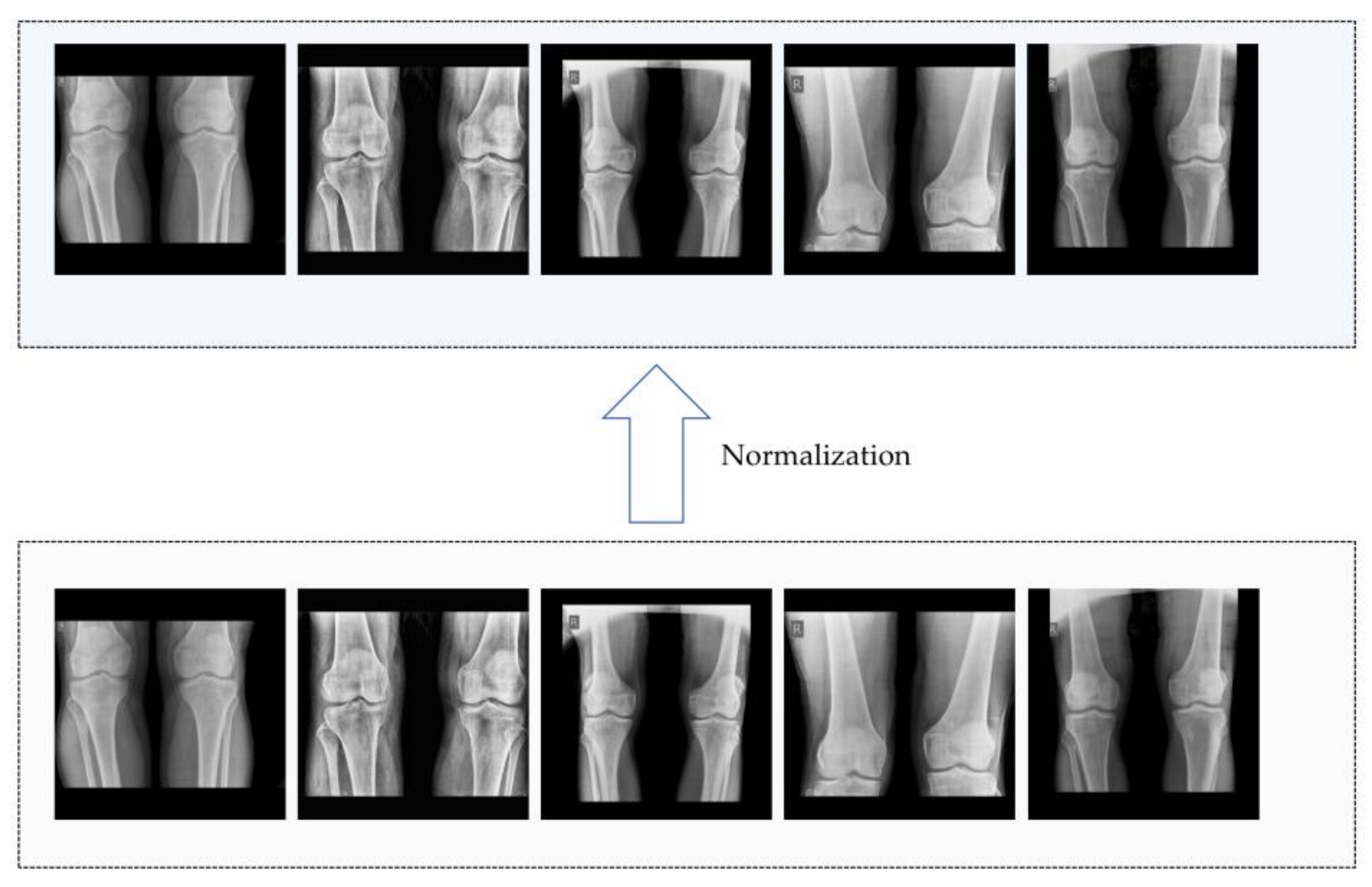
To normalize the images, they were converted to grayscale and resized to 1024 × 1024 pixels using nearest neighbor interpolation [24], which calculates the value of the target pixel with linear interpolation between the four nearest neighbor pixels in the original image. Subsequently, the max/min normalization method was applied to each image, and partial results of the normalization process are depicted in Figure 2. This normalization ensures that the medical images have a consistent grayscale representation, facilitating the detection of features within the images. Furthermore, the images were enhanced using the contrast-limited adaptive histogram equalization (CLAHE) algorithm to improve contrast and provide a clearer visualization of the feature details [25]. This approach avoids the potential problem of noise enhancement associated with the adaptive histogram equalization (AHE) method by constraining the range of contrast enhancement. The advantage of using CLAHE is that it achieves effective contrast enhancement without introducing excessive noise.

2.2.2. GLCM Feature Extraction

Accumulated evidence has provided substantial support for the effectiveness of the gray-level co-occurrence matrix (GLCM) in capturing bone architecture properties. This approach has been successfully applied in various domains, including the assessment of bone quality [26], the diagnosis of osteosarcoma [27,28,29,30], and the prediction of fractures [31]. In this study, the GLCM was computed for each sample, and significant texture features were extracted from each GLCM. These features were subsequently concatenated into a vector to represent the information within a specific ROI. The resulting ROI feature vectors were then generated and utilized as input for the FBLS model.
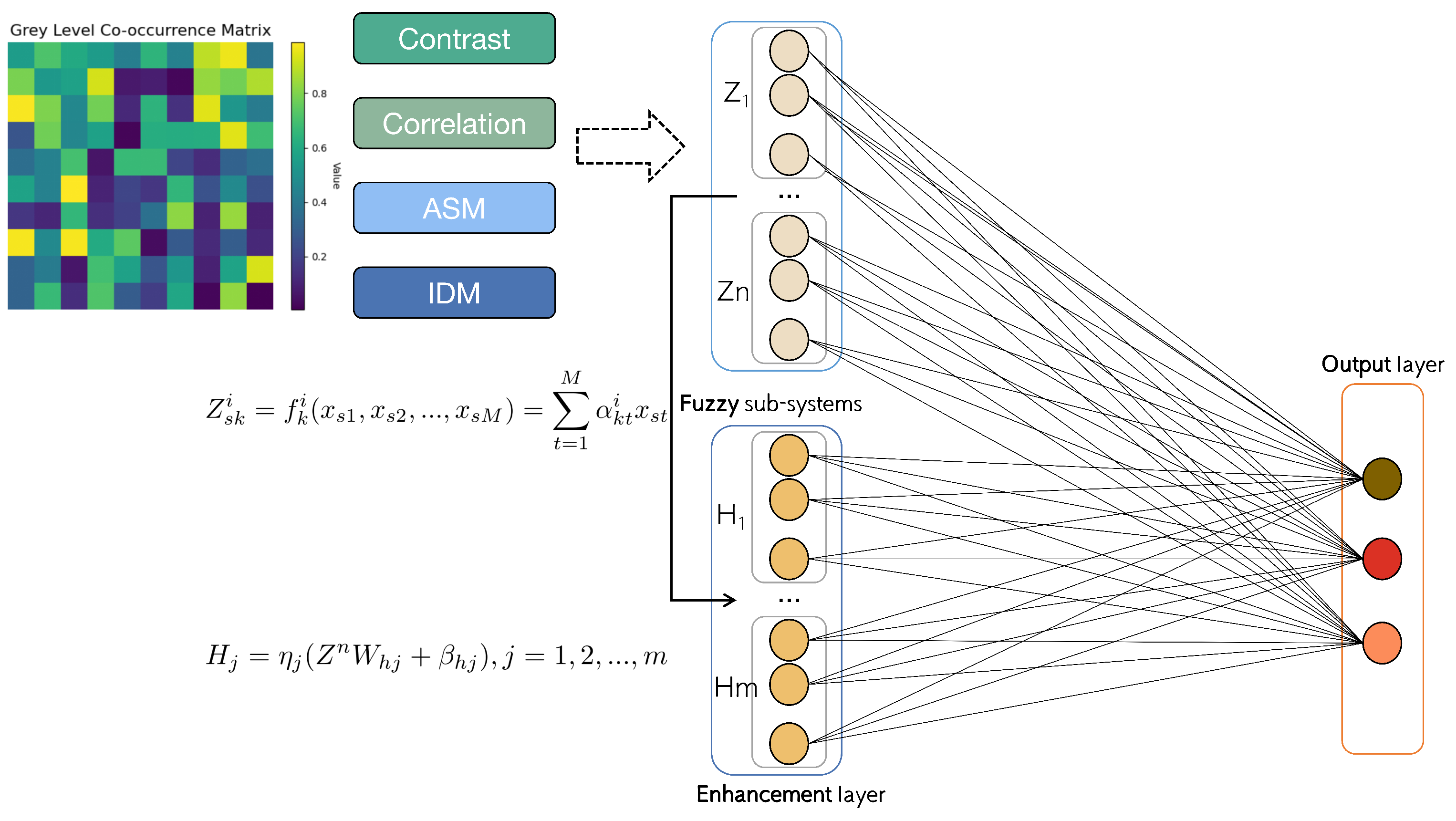
The GLCM is a mathematical representation that offers significant information about the intricate characteristics of an image. As shown in Figure 3, each element within the matrix corresponds to the statistical probabilities of changes between various gray levels at specific displacement distances and angles, commonly 0°, 45°, 90°, and 135°. For the classification task in this study, the following uncorrelated features were selected: contrast, angular second moment, inverse different moment, and correlation. The subsequent content will provide detailed explanations of these selected features.

Contrast

The contrast reflects the image clarity and depth of the grooves in the texture. The greater the contrast, the deeper the grooves. Conversely, if the contrast is small, the grooves are shallow. The contrast is obtained using the following equation:
Contrast   = i , j = 0 N 1 i j × P i , j
where N − 1 is the number of gray levels; P(i,j) is the gray-level co-occurrence matrix; i and j are the spatial coordinates of the function.

Angular Second Moment (Energy)

The ASM describes the uniformity of an image’s gray distribution. If all the element values of the GLCM are very close, the ASM value will be small. However, if the values differ greatly, the ASM will be large. The ASM is obtained using the following equation:
Energy   = i , j = 0 N 1 P i , j 2

Inverse Different Moment

The IDM reflects the change in an image’s local texture. If the textures of different regions of the image are uniform and change slowly, the inverse variance will be large; otherwise, it will be small. The IDM is obtained using the following equation:
IDM   = i , j = 0 N 1 1 / 1 + i j 2 × P i , j

Correlation

The correlation reflects the consistency of the image texture, and it measures the degree of similarity of the spatial gray-level co-occurrence matrix elements in the direction of a row or column. When the matrix element values are uniform and tend to be equal, the correlation value will be large. Conversely, if the matrix element values differ greatly, the correlation value will be small. The correlation is obtained using the following equation:
Correlation   = i , j = 0 N 1 i μ j μ × P i , j σ 2
where
μ = i , j = 0 N 1 i × P i , j
σ 2 = i , j = 0 N 01 i μ 2 × P i , j
The selected features can distinguish osteoporosis from non-osteoporosis (Table 1 and Table 2). The details of using the GLCM method to obtain these features are as follows:
Suppose that there is a medical image dataset. First, for the input data X, we select a suitable neighborhood size N × N to calculate the spatial relationship of pixel pairs in the image. Second, through Equation (7), the frequency of gray value pairs of neighboring pixels is calculated within a defined neighborhood for each pixel in one image.
GLCM i , j = [ X p , g = i , X p + d , q + θ = j ]
where i, j belong to [0, N − 1]; d and θ are predefined parameters which represent distance and direction, respectively.
Second, we normalized the gray-level co-occurrence matrix through Equation (8). Divide each element in the matrix GLCM by the sum of GLCM to eliminate the effect of image size and gray-level range on features.
P i , j = GLCM i , j , d , θ GLCM k , l , d , θ
Finally, we use Equations (1)–(4) to calculate the following four features mentioned above: contrast, energy, IDM, and correlation.
Fea = Merge Contrast , Energy , IDM , Correlation
Then, through Equation (9), these features are merged into a vector describing a single image.

2.2.3. Fuzzy Broad Learning System Architecture

The fuzzy broad learning system (FBLS) [32] is architecture based on the random vector functional link neural network and pseudo-inverse theory. This design enables the system to learn quickly and incrementally, as well as to remodel the system without the need for retraining. The FBLS model, depicted in Figure 3, consists of an input layer, a fuzzy subsystem layer, an enhancement node composite layer, and an output layer. In the composite layer, multiple groups of fuzzy subsystems are generated from the input data using fuzzy rules. These fuzzy subsystems are then enhanced as enhancement nodes, each with different random weights. The output is computed by connecting all the features and enhancement nodes to the output layer.
The main concept behind the fuzzy BLS is to map the input data into a set of fuzzy rules and then utilize the BLS algorithm to learn and optimize the weights and parameters of these rules. These fuzzy rules are composed of fuzzy sets and their corresponding membership functions, which describe the fuzzy relationship between the inputs and outputs. By employing fuzzy logic’s inference, the system can make predictions and classifications based on the fuzzy representation of the input data.
The FBLS is a neural network model that incorporates the random vector functional link neural network and pseudo-inverse theory. This design allows the system to learn and adapt quickly, without the need for retraining. As shown in Figure 3, it consists of an input layer, a fuzzy subsystem layer, an enhancement layer, and an output layer. In the fuzzy subsystem layer, multiple groups of fuzzy subsystems are generated from the input data using fuzzy rules. These fuzzy subsystems are then transformed as enhancement nodes using random weights. The output is computed by connecting all the fuzzy subsystems and enhancement nodes to the output layer.
The fuzzy rules consist of fuzzy sets and their corresponding membership functions, which describe the fuzzy relationship between the inputs and outputs. By employing fuzzy logic’s inference, the system can make predictions and classifications based on the fuzzy representation of the input data.
The specific implementation steps are as follows:
In a fuzzy BLS, suppose there are n fuzzy systems and m groups of enhancement nodes. The input features are denoted by X R N × M , where M is the dimension of each feature vector. Assume that the i th fuzzy subsystem has K i fuzzy rules of the following form.
if   x 1 is   A k 1 , x 2 is   A k 2 , ... , and   x M is   A kM then z sk i = f k i x s 1 , x s 2 , ... , x sM ,   k = 1 ,   2 , , K i
where Akj is a fuzzy set, xj is the system input (j = 1, 2, …, M), and K is the number of rules.
Then, we adopt the first-order Takagi–Sugeno (TS) fuzzy system and we let
z sk i = f k i x s 1 , x s 2 , ... , x sM = t = 1 M α kt i x st
where αikt is the coefficient. The fire strength of the k th fuzzy rule in the i th fuzzy subsystem is
τ sk i = t = 1 M μ kt i x st
Then, we denote the weighted fire strength for each fuzzy rule as
ω sk i τ sk i k = 1 K i τ sk i
The Gaussian membership function is chosen for μikt(x) that corresponds to fuzzy set Aikt, which is defined as follows:
μ kt i x = e x c kt i σ kt i 2
where cikt and σikt are width and center, respectively.
In the FBLS, fuzzy subsystems deliver the intermediate vectors to the enhancement layer, which performs a further non-linear modification while retraining the input features. The intermediate vector xs, without aggregation in the i th fuzzy subsystem, is
Z si = ω s 1 i z s 1 i , ω s 2 i z s 2 i , ... , ω sK i i z sK i i
For all training samples X, the i th fuzzy subsystem’s output matrix is
Z i = Z 1 , Z 2 , ... , Z n ϵ R N × K i , i = 1 ,   2 , , n
Then, we designate an intermediate output matrix for n fuzzy subsystems by
Z n = Z 1 , Z 2 , ... , Z n ϵ R N × K 1 + K 1 + ... + K n
Then, Zn is passed to the enhancement layer for further non-linear processing. Consider the j th enhancement node group to be made up of Lj neurons represented by
H j = δ j Z n W h j + b h j ϵ R N × L j
where Whj and bhj are the j th enhancement node group’s random weights and bias terms, respectively. The enhancement layer’s output matrix is
H j = H 1 , H 2 , ... , H m
We now consider the output of each fuzzy subsystem, a process known as defuzzification. The defuzzification output Fn and the enhancement layer output matrix Hm will then be combined and sent to the top layer. First, consider the j th fuzzy subsystem’s output vector.
F si = k = 1 K i ω sk i t = 1 M φ k 1 i α kt i x st , ... , k = 1 K i ω sk i t = 1 M φ kC i α kt i x st = t = 1 M α kt i x st ω s 1 i , ... , ω sK i i φ 11 i φ 1 C i φ K i 1 i φ K i C i
where φ kC i is a new parameter in the FBLS. To reduce the number of parameters, we convert α kt i to φ kC i α kt i and calculate the pseudo-inverse. For all fuzzy subsystems, we set
D = diag t = 1 M α kt i x 1 t , ... , t = 1 M α kt i x Nt
π i = ω 11 i ω 1 K i i ω N 1 i ω NK i i
φ i = φ 11 i φ 1 C i φ K i 1 i φ K iC i
The three terms are then combined and rewritten as F. The output of i th fuzzy subsystem for the input data X is
F i = F 1 i , F 2 i , ... , F Ni T D π i φ i ϵ R N × C
The top layer’s aggregate output of n fuzzy subsystems can then be obtained as follows:
F n = i = 1 n F i = i = 1 n D π i φ i
Now consider the top layer. We send the value of defuzzification Fn, which is related to the output of the enhancement layer Hm and is connected to the weight matrix of the enhancement layer, denoted as We ∈ R(L1+L2+Lm)×C, to the top layer of the FBLS. As a result, the FBLS final output is equal to 2.
Y ^ = F n + H m W e = D π φ + H m W e = D π , H m W
W denotes the parameter matrix of a fuzzy BLS. W can be quickly calculated via the pseudo-inverse given training targets Y.
W = D π , H m + Y = D π , H m T D π , H m 1 D π , H m T
A certain number of features and enhancement nodes are selected in advance to train the BLS model. The parameters’ range for selectionis 10–20 for the number of enhancement node groups and 10–50 for the number of feature node groups. Suitable parameters are selected from these ranges to enhance the robustness of the model.

3. Results

3.1. State-of-the-Art CNN Models for Automatic Screening of Athletes Osteopenia and Osteoporosis

Deep learning (DL) models have made significant advancements in the field of osteoporosis screening [33,34,35,36]. ResNet, DenseNet, and EfficientNet are among the most widely utilized State-of-the-Art DL models for osteoporosis screening and have demonstrated impressive performance in screening tasks. EfficientNet is particularly renowned for its ability to achieve excellent classification results while also being computationally efficient. This is achieved through the combination of depthwise separable convolution and residual connection techniques, which effectively reduce computational costs. Consequently, several studies have proposed the use of EfficientNet for osteoporosis screening [37,38,39]. On the other hand, ResNet focuses on learning the residual between the input and the desired output. By formulating the problem as learning residuals, the network can learn the incremental changes necessary to improve the representation. Due to its robust representation capability, ResNet and its variants have been widely adopted for osteoporosis screening using various types of datasets, such as knee X-rays, musculoskeletal radiographs, and panoramic radiographs [40,41,42]. DenseNet, on the other hand, introduces dense connectivity, where each layer is directly connected to every other layer in a feed-forward manner. This dense connectivity allows for maximum information flow between layers, enabling feature reuse and facilitating gradient propagation throughout the network. As a result, DenseNet has demonstrated great performance in osteopenia and osteoporosis screening [43,44].
These three DL models are widely applied in the screening of osteopenia and osteoporosis. Consequently, when compared to these models, our proposed GLCM-based FBLS can be validated as a viable alternative to DL-based methods for screening osteoporosis and osteopenia.

3.1.1. ResNet

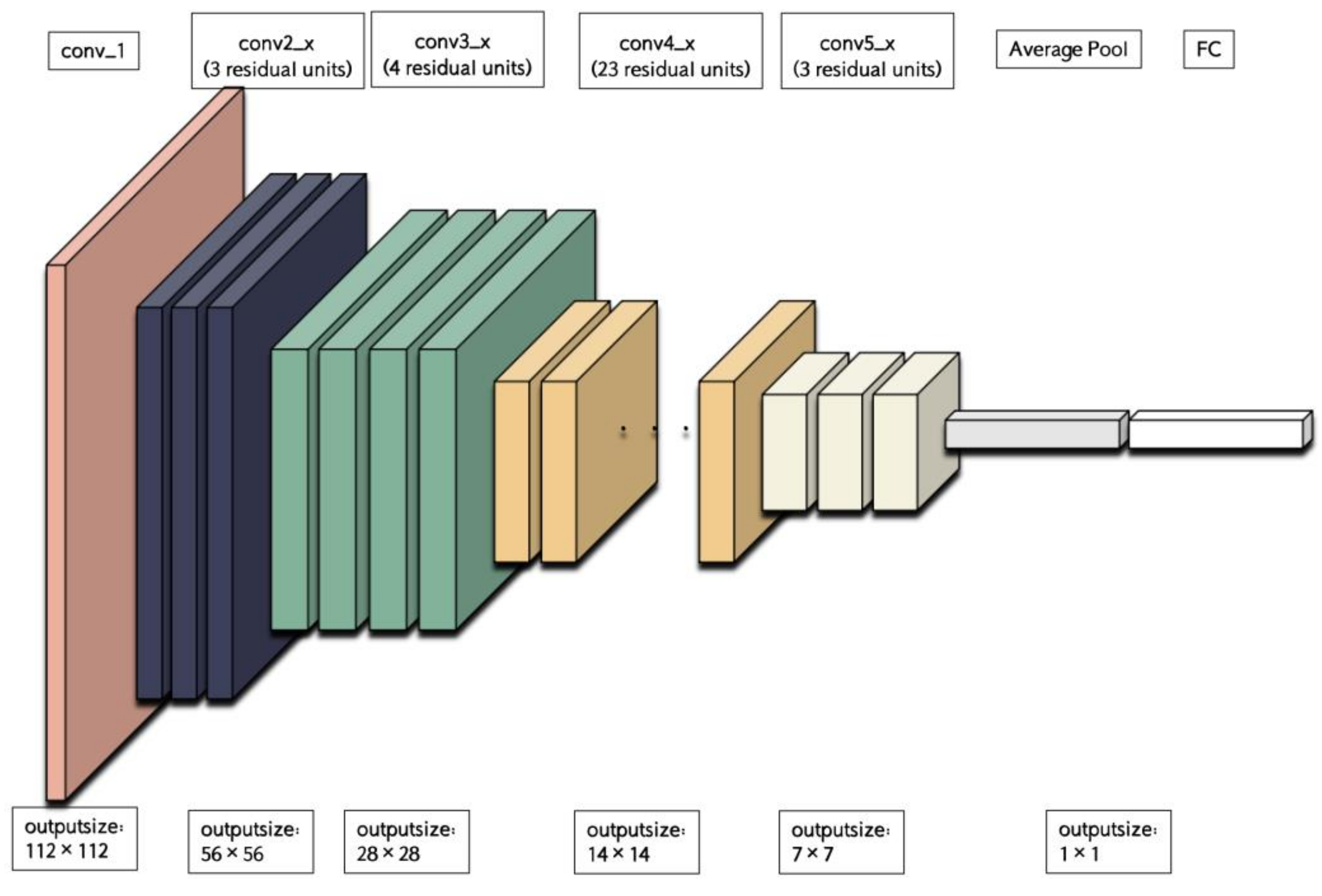
ResNet (Residual Network) is a deep neural network architecture that has gained significant popularity in the field of computer vision. It is designed based on the concept of residual learning, which enables the network to learn residual mappings instead of directly learning the underlying mapping. This approach has proven to be effective in mitigating the vanishing gradient problem commonly encountered in deep neural networks, thereby enabling the training of much deeper networks. In this study, we have specifically chosen ResNet-101, which consists of five convolutional groups. As shown in Figure 4, the first group comprises a single basic convolutional operation, with each operation consisting of a convolutional layer with a kernel size of 7 × 7, a batch normalization layer, and a ReLU layer. ReLU, short for Rectified Linear Unit, is a widely used activation function in deep learning. It is defined as f(x) = max(0, x), where x represents the input value and f(x) represents the resulting output. The primary purpose of the ReLU layer is to introduce non-linearity, enabling the model to learn intricate patterns and relationships within the data. By utilizing ReLU as an activation function, deep learning models can effectively capture complex features and enhance their representation capabilities. The second to fifth convolutional groups consist of 3, 4, 23, and 3 residual units, respectively, with each unit containing three convolutional layers (with kernel sizes of 1 × 1, 3 × 3, and 1 × 1, respectively). Each convolutional group performs a downsampling operation at the end, reducing the size of the feature map by half. Subsequently, through average downsampling, a fully connected layer, and a softmax function layer, the classification results can be obtained.
Several studies have utilized ResNet for the automatic screening of osteoporosis using radiographs. For instance, Melek Tassoker et al. evaluated the performance of ResNet on panoramic radiographs and achieved a sensitivity of 76.52%, specificity of 87.37%, and accuracy of 75.08% in detecting osteoporosis and osteopenia [40]. I. M. Wani et al. employed ResNet with transfer learning techniques to diagnose osteoporosis based on knee X-ray images, achieving an accuracy of 74.3% after 10 training epochs [41]. Additionally, Bhan A et al. applied ResNet to detect osteoporosis in musculoskeletal radiographs, achieving an area under the curve (AUC) of 89.23% and an accuracy of 86.49% [42]. The residual module in ResNet enables it to learn residual mappings, thereby capturing complex patterns and representations within the image. However, the deeper architecture and residual connections of ResNet increase the computational complexity and memory requirements during both training processes.

3.1.2. DenseNet

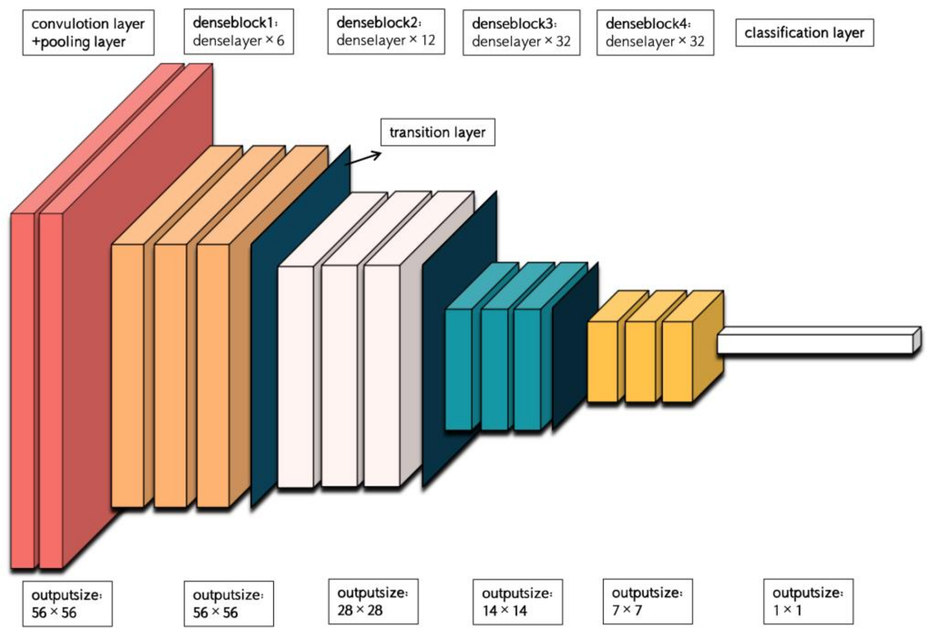
DenseNet (Densely Connected Convolutional Network) is a deep neural network architecture, which is designed based on the concept of densely connecting each layer to every other layer in a feedforward manner. This connectivity pattern allows for efficient information flow and feature reuse throughout the network. The architecture of DenseNet-169 is depicted in Figure 5. DenseNet-169 consists of a conventional layer with a kernel size of 7 × 7, a pooling layer with a size of 3 × 3 for maximum pooling, four dense blocks with a transition layer between each pair of blocks, and a classification layer. Each dense block contains multiple conventional groups, which are composed of two conventional layers with kernel sizes of 1 × 1 and 3 × 3. The four dense blocks have different numbers of conventional groups, specifically 6, 12, 32, and 32. The transition layer is responsible for reducing computational complexity and consists of a conventional layer with a kernel size of 1 × 1 and a pooling layer with a size of 2 × 2 for average pooling. Finally, the classification layer includes a pooling layer with a size of 7 × 7 for global average pooling, a fully connected layer, and a softmax function layer to obtain the final result.
DenseNet has been applied in various studies for the automatic screening of osteoporosis using radiographs. For instance, researchers proposed a 3D DenseNet model for the detection of osteoporotic vertebral compression fractures. The model achieved high sensitivity (95.7%) and specificity (92.6%), as well as positive predictive value (PPV) of 91.7% and negative predictive value (NPV) of 96.2% [43]. Another study conducted by Tang et al. utilized a novel convolutional neural network (CNN) model based on DenseNet to qualitatively detect bone mineral density for osteoporosis screening [44]. The classification precision for normal bone mass, low bone mass, and osteoporosis was reported as 80.57%, 66.21%, and 82.55%, respectively. The AUC exhibited a similar distribution pattern as the precision. The dense connectivity in DenseNet enables direct access to feature maps from all preceding layers, facilitating feature reuse and enhancing the network’s ability to learn and utilize feature information, thereby improving classification performance. However, the dense connection mechanism of DenseNet leads to increased computational complexity as each layer needs to connect with all previous layers. Moreover, DenseNet requires a significant amount of memory to store numerous feature maps, which can pose memory limitations when working with large medical datasets.

3.1.3. EfficientNet

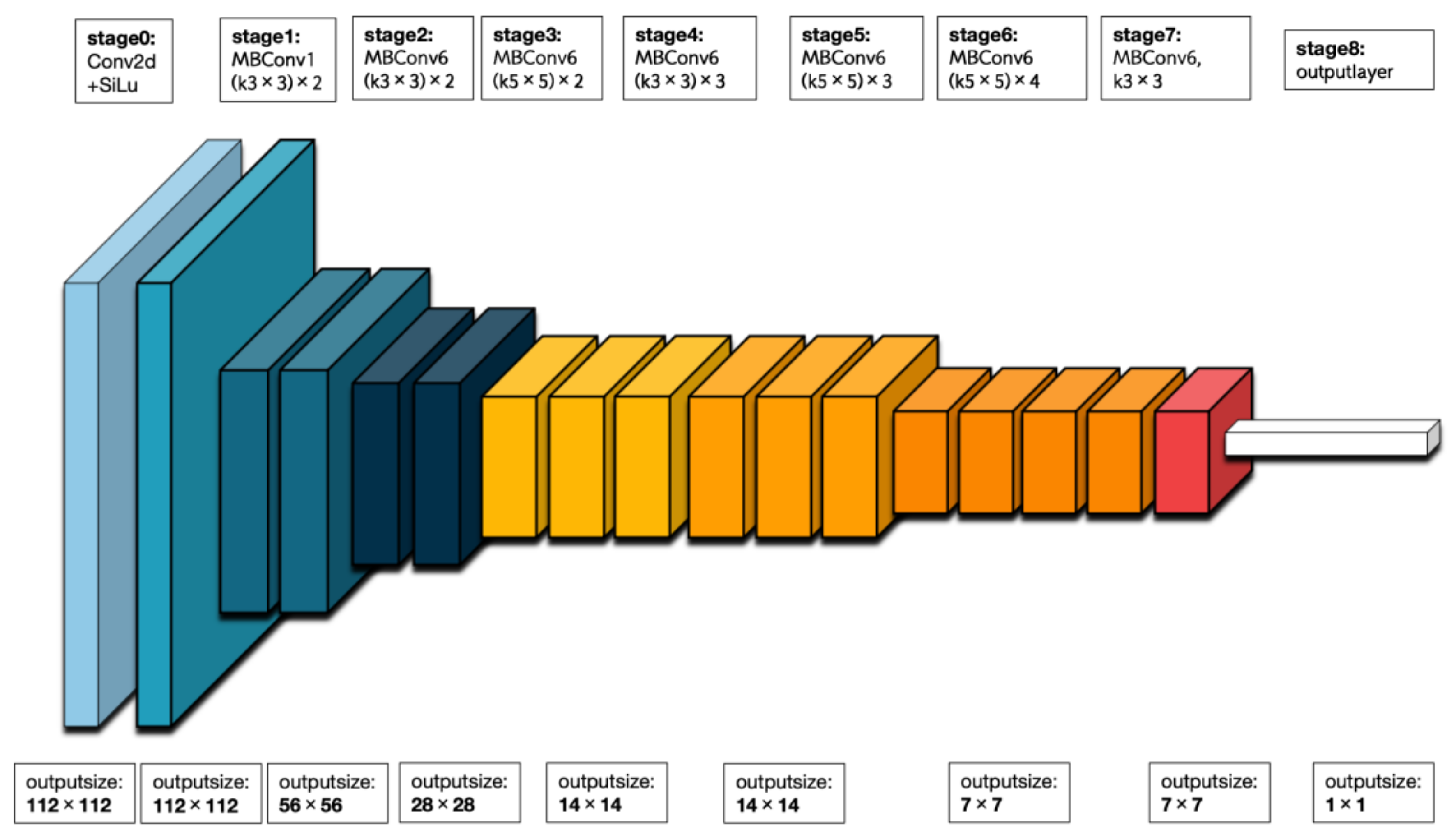
EfficientNet is a family of deep neural network architectures. These architectures are constructed using a compound scaling method that simultaneously scales up the depth, width, and resolution of the network. Among the variants of EfficientNet, EfficientNet-B0 is the smallest, possessing fewer parameters and lower computational complexity compared to its larger counterparts. Figure 6 illustrates the division of EfficientNet-B0 into nine stages. The initial stage consists of a standard convolutional layer with a kernel size of 3 × 3, including batch normalization (BN) and the Swish activation function. Stages 2 to 8 involve the repetition of MBConv structures, while stage 9 comprises an ordinary 1 × 1 convolutional layer (including BN and Swish), an average pooling layer, a fully connected layer, and a softmax function layer. The MBConv structure itself consists of a 1 × 1 ordinary convolutional operation (which raises the dimensionality, including BN and Swish), a k × k (3 × 3 or 5 × 5) depthwise convolution (including BN and Swish), an SE module, a 1 × 1 ordinary convolution (which reduces dimensionality, including BN), and a dropout layer.
EfficientNet has been utilized in various studies for the automatic screening of osteoporosis using radiographs. For instance, Norio Yamamoto et al. evaluated the predictive ability of EfficientNet on hip radiographs and achieved a sensitivity of 82.26%, specificity of 92.16%, and an AUC of 92.19% [37]. Usman Bello Abubakar et al. employed EfficientNet with fine-tuning techniques to classify osteoporosis in knee radiographs, achieving a sensitivity and specificity of 86% [39]. EfficientNet effectively manages model complexity and computational costs through composite scaling factors, while still maintaining high performance. It can achieve performance comparable to larger models with smaller model sizes. However, it is important to note that EfficientNet’s high performance often relies on the availability of large training datasets and ample computing resources. In the context of osteoporosis classification, if the training dataset is limited or computational resources are constrained, it may have an impact on the training and performance of the model.

3.2. Experimental Settings

We compared the BLS model with ResNet-101, DenseNet-169, and EfficientNet-B0. For these three CNN models, we used Adaptive Moment Estimation as our optimizer and set the learning rate of ResNet-101, DenseNet-169, and EfficientNet-B0 to 0.1, 0.01, and 0.001 with a batch size of 32.
The BLS and CNN models were implemented using MATLAB R2021b (The MathWorks Inc., Natick, MA, USA) and Pycharm CE (JetBrains, PyCharm 2020.1.2). All analyses were performed under Google Collaboratory on a machine with a graphics processing unit (GPU) with a Driver Version 460.32.03 and CUDA Version 11.2.

3.3. Results Analysis

Table 3 and Figure 7 present the diagnostic performances of the GLCM-based FBLS and CNN models in distinguishing osteoporosis, osteopenia, and non-findings in each cohort. Additionally, we indicated the experimental results on the trained cohort to demonstrate that every model has successfully avoided overfitting. From Table 3, we can see that GLCM-based FBLS achieved a 2.90% increase in AUC, 6.55% increase in accuracy, 11.31% increase in specificity, and 7.38% increase in NPV. The performance results demonstrate that the proposed GLCM-based FBLS can provide athletes with accurate screening of osteopenia and osteoporosis, especially in classifying those with no findings.
However, the proposed model does not perform well in terms of sensitivity and PPV. After careful study, we believe that there is a large overlap between the samples of osteoporosis and osteopenia, which are different stages of the disease. It limits the model’s performance when classifying the different stages of osteoporosis. Nevertheless, our model has shown considerable advantages in terms of AUC, accuracy, specificity, and NPV, demonstrating its potential in accurately determining whether athletes are suffering from osteoporosis. In our future work, we will further focus on improving the ability of the proposed model to screen for different conditions of osteoporosis, hoping to completely improve this problem in the future.

4. Discussion

We have developed and validated a novel artificial intelligence method called the GLCM-based FBLS, which combines gray-level co-occurrence matrix with fuzzy BLS. This method considers the texture information of X-ray images and utilizes fuzzy systems to enhance the robustness of the BLS model. Our experimental results demonstrate that this method is effective and efficient in detecting osteoporosis and osteopenia.
Osteoporosis is a significant concern for athletes as it can have a detrimental impact on their health and athletic performance. It can lead to weakened bones and increased susceptibility to fractures, which can hinder an athlete’s ability to train and compete. Currently, conventional screening strategies for osteoporosis, such as calcaneal quantitative ultrasonography (QUS), quantitative computed tomography (QCT), and magnetic resonance imaging (MRI) [45], are not widely used due to limitations such as high radiation doses and complex post-processing. This makes it challenging to incorporate these strategies into regular screening for athletes. Opportunistic osteoporosis screening using machine learning models based on X-ray images may be a more efficient approach, as X-ray images are widely available for training the model. Previous studies have applied various machine learning models to analyze, predict, and diagnose osteoporosis and osteopenia. Deep learning algorithms have also been utilized, achieving significant progress in the detection of osteoporosis. However, these deep learning methods are computationally intensive and lack interpretability.
In contrast, our proposed GLCM-based FBLS method offers advantages in terms of its lightweight nature and ease of training compared to deep learning models. By utilizing the GLCM-based feature extraction method, complex information in images can be transformed into texture information, resulting in reduced noise. The incorporation of fuzzy systems in the FBLS allows for handling uncertainty and imprecision in data, resulting in robust and reliable results. Our experimental results demonstrate that our method outperforms traditional CNN models on various indices. Therefore, our proposed model shows promise in achieving more accurate and reliable results in osteoporosis screening for athletes, particularly in determining the presence of the disease. Additionally, the lightweight nature of our model enhances its portability and eliminates the need for storing a large number of parameters and features. Moreover, our model enables fast and accurate predictions directly from X-ray images, offering potential for integration with the daily examination of athletes.
However, our study has several limitations that should be acknowledged. Firstly, it was a retrospective study with a relatively small sample size. Future prospective studies are needed to validate the generalization ability of the BLS model. Secondly, our study focused on a classification task rather than a regression task, aiming to predict BMD T-scores categories rather than exact values. This decision was made due to the complex non-linear relationship between knee bones and BMD T-scores, which poses challenges for regression modeling. Thirdly, to apply the proposed method to real-world scenarios, adjustments may be necessary in the fuzzy rules used in the FBLS algorithm to enhance its performance. Lastly, we did not evaluate the potential contribution of clinical factors, such as age and body mass index, to the AI models. Although a recent study found that demographic characteristics did not significantly improve the sensitivity of osteoporosis identification, another study suggested that biochemical indicators could enhance the accuracy of an image-based model.

5. Conclusions

We have developed and validated a novel FBLS for the purpose of screening osteoporosis in athletes. This model utilizes GLCM features extracted from knee X-ray images as input data, which significantly reduces redundant information and noises. The GLCM features are then combined with the fuzzy broad learning system, which is advantageous in handling uncertainty and imprecision in the extracted features. Our findings demonstrate that the proposed model is an effective and efficient method for diagnosing osteoporosis, surpassing the performance of traditional CNN models. Additionally, the GLCM-based FBLS model produces diagnosis results that are more easily interpretable compared to the CNN-based models.
The fuzzy rules in the FBLS, which consist of fuzzy sets and their corresponding membership functions, enable our model to extract critical information from the fuzzy relationship among the extracted features. Furthermore, the proposed model has a simple flat structure and does not require retraining processes, which also facilitates feature representation learning and data classification. Moreover, the FBLS weights are determined using analytical computation, reducing the risk of model overfitting and enhancing generalization ability compared to the CNN models.

Author Contributions

Conceptualization, Z.C. and H.Z.; methodology, Z.C.; software, Z.C.; validation, Z.C.; formal analysis, Z.C.; investigation, H.Z.; resources, Z.C.; data curation, Z.C.; writing—original draft preparation, Z.C.; writing—review and editing, Z.C. and J.D.; visualization, Z.C.; supervision, X.W. and J.D.; project administration, X.W. and J.D.; funding acquisition, X.W. All authors have read and agreed to the published version of the manuscript.

Funding

This research was funded by Civilized Guangzhou and Cultural Power Research Base 2023 research project, grant number 2023JDGJ09.

Informed Consent Statement

Informed consent was obtained from all subjects involved in this study.

Data Availability Statement

The link of the dataset in this manuscript is as follows: https://data.mendeley.com/datasets/fxjm8fb6mw (accessed on 15 July 2023).

Acknowledgments

Thanks to Yifeng Lin from College of Cyber Security, Jinan University and Yuer Yang from Department of Computer Science, The University of Hong Kong, for providing submission information.

Conflicts of Interest

The authors declare no conflict of interest.

References

  1. Compston, J.E.; McClung, M.R.; Leslie, W.D. Osteoporosis. Lancet 2019, 393, 364–376. [Google Scholar] [CrossRef] [PubMed]
  2. Broken Bones. Broken Lives: A Roadmap to Solve the Fragility Fracture Crisis in Europe; International Osteoporosis Foundation: Nyon, Switzerland, 2018. [Google Scholar]
  3. Anil, G.; Guglielmi, G.; Peh, W.C.G. Radiology of osteoporosis. Radiol. Clin. 2010, 48, 497–518. [Google Scholar] [CrossRef] [PubMed]
  4. Lim, H.K.; Ha, H.I.; Park, S.Y.; Han, J. Prediction of femoral osteoporosis using machine-learning analysis with radiomics features and abdomenpelvic CT: A retrospective single center preliminary study. PLoS ONE 2021, 16, e0247330. [Google Scholar]
  5. Sebro, R.; Elmahdy, M. Machine learning for opportunistic screening for osteoporosis and osteopenia using knee CT scans. Can. Assoc. Radiol. J. 2023. [Google Scholar] [CrossRef] [PubMed]
  6. Park, H.W.; Jung, H.; Back, K.Y.; Choi, H.J.; Ryu, K.S.; Cha, H.S.; Lee, E.K.; Hong, A.R.; Hwangbo, Y. Application of machine learning to identify clinically meaningful risk group for osteoporosis in individuals under the recommended age for dual-energy X-ray absorptiometry. Calcif. Tissue Int. 2021, 109, 645–655. [Google Scholar] [CrossRef] [PubMed]
  7. Krizhevsky, A.; Sutskever, I.; Hinton, G.E. Imagenet classification with deep convolutional neural networks. In Proceedings of the Advances in Neural Information Processing Systems, Lake Tahoe, NV, USA, 3–6 December 2012; Volume 25. [Google Scholar]
  8. Fang, Y.; Li, W.; Chen, X.; Chen, K.; Kang, H.; Yu, P.; Zhang, R.; Liao, J.; Hong, G.; Li, S. Opportunistic osteoporosis screening in multi-detector ct images using deep convolutional neural networks. Eur. Radiol. 2021, 31, 1831–1842. [Google Scholar] [CrossRef] [PubMed]
  9. Pickhardt, P.J.; Nguyen, T.; Perez, A.A.; Graffy, P.M.; Jang, S.; Summers, R.M.; Garrett, J.W. Improved ct-based osteoporosis assessment with a fully automated deep learning tool. Radiol. Artif. Intell. 2022, 4, e220042. [Google Scholar] [CrossRef] [PubMed]
  10. Tomita, N.; Cheung, Y.Y.; Hassanpour, S. Deep neural networks for automatic detection of osteoporotic vertebral fractures on ct scans. Comput. Biol. Med. 2018, 98, 8–15. [Google Scholar] [CrossRef]
  11. Wu, G.; Duan, J. Blcov: A novel collaborative–competitive broad learning system for covid-19 detection from radiology images. Eng. Appl. Artif. Intell. 2022, 115, 105323. [Google Scholar] [CrossRef]
  12. Chen, C.L.P.; Liu, Z. Broad learning system: An effective and efficient incremental learning system without the need for deep architecture. IEEE Trans. Neural Netw. Learn. Syst. 2017, 29, 10–24. [Google Scholar] [CrossRef]
  13. Zebari, R.; Abdulazeez, A.; Zeebaree, D.; Zebari, D.; Saeed, J. A comprehensive review of dimensionality reduction techniques for feature selection and feature extraction. J. Appl. Sci. Technol. Trends 2020, 1, 56–70. [Google Scholar] [CrossRef]
  14. Zulpe, N.; Pawar, V. Glcm textural features for brain tumor classification. Int. J. Comput. Sci. Issues (IJCSI) 2012, 9, 354. [Google Scholar]
  15. Wilson, D.J. Osteoporosis and sport. Eur. J. Radiol. 2019, 110, 169–174. [Google Scholar] [CrossRef]
  16. Adams, J.E. Advances in bone imaging for osteoporosis. Nat. Rev. Endocrinol. 2013, 9, 28–42. [Google Scholar] [CrossRef] [PubMed]
  17. Schousboe, J.T.; Ensrud, K.E. Opportunistic osteoporosis screening using low-dose computed tomography (ldct): Promising strategy, but challenges remain. J. Bone Miner. Res. 2021, 36, 425–426. [Google Scholar] [CrossRef] [PubMed]
  18. Mithal, A.; Ebeling, P. International Osteoporosis Foundation. The Asian Pacific Regional Audit: Epidemiology, Costs & Burden of Osteoporosis in 2013; International Osteoporosis Foundation: Nyon, Switzerland, 2013. [Google Scholar]
  19. He, K.; Zhang, X.; Ren, S.; Sun, J. Deep residual learning for image recognition. In Proceedings of the IEEE Conference on Computer Vision and Pattern Recognition, Las Vegas, NV, USA, 27–30 June 2016; pp. 770–778. [Google Scholar]
  20. Tan, M.; Le, Q. Efficientnet: Rethinking model scaling for convolutional neural networks. In Proceedings of the International Conference on Machine Learning, Long Beach, CA, USA, 10–15 June 2019; pp. 6105–6114. [Google Scholar]
  21. Iandola, F.; Moskewicz, M.; Karayev, S.; Girshick, R.; Darrell, T.; Keutzer, K. Densenet: Implementing efficient convnet descriptor pyramids. arXiv 2014, arXiv:1404.1869. [Google Scholar]
  22. Chawla, N.V.; Bowyer, K.W.; Hall, L.O.; Kegelmeyer, W.P. Smote: Synthetic minority over-sampling technique. J. Artif. Intell. Res. 2002, 16, 321–357. [Google Scholar] [CrossRef]
  23. Wani, I.M.; Arora, S. Knee X-ray Osteoporosis Database. Mendeley Data 2021. [Google Scholar] [CrossRef]
  24. Gonzales, R.C.; Woods, R.E.; Eddins, S.L. Digital Image Processing Using MATLAB; Pearson Prentice Hall: Hoboken, NJ, USA, 2004. [Google Scholar]
  25. Zuiderveld, K. Contrast limited adaptive histogram equalization. In Graphics Gems; Elsevier: Amsterdam, The Netherlands, 1994; pp. 474–485. [Google Scholar]
  26. Shirvaikar, M.; Huang, N.; Dong, X.N. The measure- ment of bone quality using gray level co-occurrence matrix textural fea- tures. J. Med. Imaging Health Inform. 2016, 6, 1357–1362. [Google Scholar] [CrossRef]
  27. Hu, S.; Xu, C.; Guan, W.; Tang, Y.; Liu, Y. Texture feature extraction based on wavelet transform and gray-level co-occurrence matrices applied to osteosarcoma diagnosis. Biomed. Mater. Eng. 2014, 24, 129–143. [Google Scholar] [CrossRef]
  28. Areeckal, A.S.; Kamath, J.; Zawadynski, S.; Kocher, M. Combined radiogrammetry and texture analysis for early diagnosis of osteoporosis using indian and swiss data. Comput. Med. Imaging Graph. 2018, 68, 25–39. [Google Scholar] [CrossRef] [PubMed]
  29. Kawashima, Y.; Fujita, A.; Buch, K.; Li, B.; Qureshi, M.M.; Chapman, M.N.; Sakai, O. Using textureanalysis of head ct images to differentiate osteoporosis from normal bone density. Eur. J. Radiol. 2019, 116, 212–218. [Google Scholar] [CrossRef] [PubMed]
  30. Mookiah, M.R.K.; Rohrmeier, A.; Dieckmeyer, M.; Mei, K.; Kopp, F.K.; Noel, P.B.; Kirschke, J.S.; Baum, T.; Subburaj, K. Feasibility of opportunistic osteo- porosis screening in routine contrast-enhanced multi detector computed tomography (mdct) using texture analysis. Osteoporos. Int. 2018, 29, 825–835. [Google Scholar] [CrossRef] [PubMed]
  31. Nardone, V.; Tini, P.; Croci, S.; Carbone, S.F.; Sebaste, L.; Carfagno, T.; Battaglia, G.; Pastina, P.; Rubino, G.; Mazzei, M.A.; et al. 3d bone texture analysis as a potential predictor of radiation-induced insufficiency fractures. Quant. Imaging Med. Surg. 2018, 8, 14. [Google Scholar] [CrossRef] [PubMed]
  32. Feng, S.; Chen, C.L.P. Fuzzy broad learning system: A novel neuro-fuzzy model for regression and classification. IEEE Trans. Cybern. 2018, 50, 414–424. [Google Scholar] [CrossRef] [PubMed]
  33. Jang, M.; Kim, M.; Bae, S.J.; Lee, S.H.; Koh, J.M.; Kim, N. Opportunistic Osteoporosis Screening Using Chest Radiographs with Deep Learning: Development and External Validation With a Cohort Dataset. J. Bone Miner. Res. 2022, 37, 369–377. [Google Scholar] [CrossRef] [PubMed]
  34. Jang, R.; Choi, J.H.; Kim, N.; Chang, J.S.; Yoon, P.W.; Kim, C.H. Prediction of osteoporosis from simple hip radiography using deep learning algorithm. Sci. Rep. 2021, 11, 19997. [Google Scholar] [CrossRef] [PubMed]
  35. Mao, L.; Xia, Z.; Pan, L.; Chen, J.; Liu, X.; Li, Z.; Yan, Z.; Lin, G.; Wen, H.; Liu, B. Deep learning for screening primary osteopenia and osteoporosis using spine radiographs and patient clinical covariates in a Chinese population. Front. Endocrinol. 2022, 13, 971877. [Google Scholar] [CrossRef]
  36. Xie, Q.; Chen, Y.; Hu, Y.; Zeng, F.; Wang, P.; Xu, L.; Wu, J.; Li, J.; Zhu, J.; Xiang, M.; et al. Development and validation of a machine learning-derived radiomics model for diagnosis of osteoporosis and osteopenia using quantitative computed tomography. BMC Med. Imaging 2022, 22, 140. [Google Scholar] [CrossRef]
  37. Yamamoto, N.; Sukegawa, S.; Kitamura, A.; Goto, R.; Noda, T.; Nakano, K.; Takabatake, K.; Kawai, H.; Nagatsuka, H.; Kawasaki, K.; et al. Deep learning for osteoporosis classification using hip radiographs and patient clinical covariates. Biomolecules 2020, 10, 1534. [Google Scholar] [CrossRef]
  38. Hempe, H.; Yilmaz, E.B.; Meyer, C.; Heinrich, M.P. Opportunistic CT screening for degenerative deformities and osteoporotic fractures with 3D DeepLab. In Medical Imaging 2022: Image Processing; SPIE: Bellingham, DC, USA, 2022; Volume 12032, pp. 127–134. [Google Scholar]
  39. Abubakar, U.B.; Boukar, M.M.; Adeshina, S. Evaluation of Parameter Fine-Tuning with Transfer Learning for Osteoporosis Classification in Knee Radiograph. Int. J. Adv. Comput. Sci. Appl. 2022, 13, 246–252. [Google Scholar] [CrossRef]
  40. Tassoker, M.; Öziç, M.Ü.; Yuce, F. Comparison of five convolutional neural networks for predicting osteoporosis based on mandibular cortical index on panoramic radiographs. Dentomaxillofacial Radiol. 2022, 51, 20220108. [Google Scholar] [CrossRef] [PubMed]
  41. Wani, I.M.; Arora, S. Osteoporosis diagnosis in knee X-rays by transfer learning based on convolution neural network. Multimed. Tools Appl. 2023, 82, 14193–14217. [Google Scholar] [CrossRef]
  42. Bhan, A.; Singh, S.; Vats, S.; Mehra, A. Ensemble Model based Osteoporosis Detection in Musculoskeletal Radiographs. In Proceedings of the 13th International Conference on Cloud Computing, Data Science & Engineering (Confluence), Noida, India, 19–20 January 2023; IEEE: Piscataway, NJ, USA, 2023; pp. 523–528. [Google Scholar]
  43. Niu, X.; Yan, W.; Li, X.; Huang, Y.; Chen, J.; Mu, G.; Li, J.; Jiao, X.; Zhao, Z.; Jing, W.; et al. A deep-learning system for automatic detection of osteoporotic vertebral compression fractures at thoracolumbar junction using low-dose computed tomography images. Res. Sq. 2022. [Google Scholar] [CrossRef]
  44. Tang, C.; Zhang, W.; Li, H.; Li, L.; Li, Z.; Cai, A.; Wang, L.; Shi, D.; Yan, B. CNN-based qualitative detection of bone mineral density via diagnostic CT slices for osteoporosis screening. Osteoporos. Int. 2021, 32, 971–979. [Google Scholar] [CrossRef] [PubMed]
  45. Damilakis, J.; Maris, T.G.; Karantanas, A.H. An update on the assessment of osteoporosis using radiologic techniques. Eur. Radiol. 2007, 17, 1591–1602. [Google Scholar] [CrossRef]
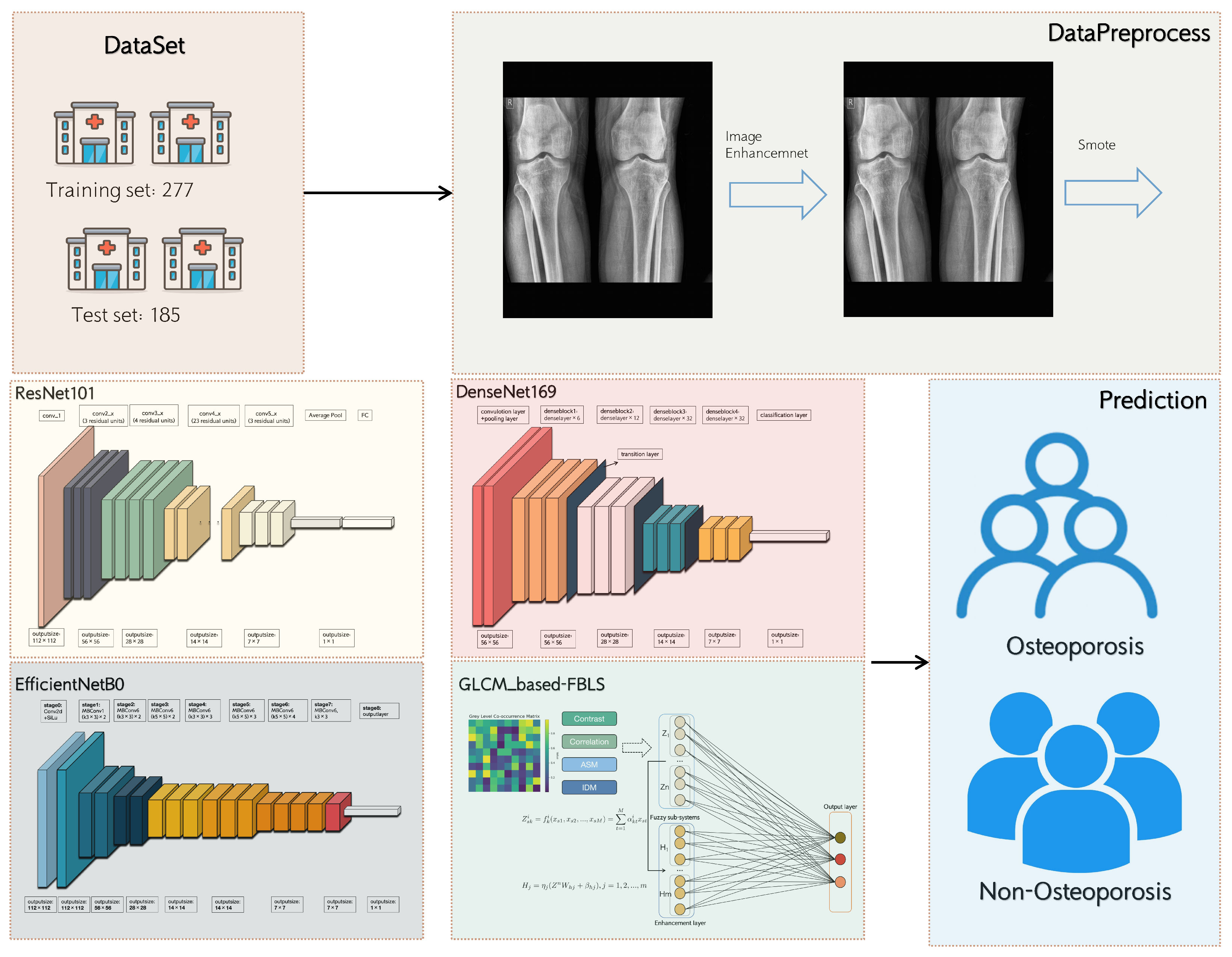
Figure 1. Schematic of the analysis plan.
Applsci 13 11150 g001
Figure 2. Part of results of normalization.
Applsci 13 11150 g002
Figure 3. The network architecture of GLCM-based BLS.
Applsci 13 11150 g003
Figure 4. The backbone of ResNet101.
Applsci 13 11150 g004
Figure 5. The backbone of DenseNet-169.
Applsci 13 11150 g005
Figure 6. The backbone of EfficientNet-B0.
Applsci 13 11150 g006
Figure 7. Performance comparison of GLCM-based FBLS and three CNN models for testing set and training set.
Applsci 13 11150 g007
Table 1. Comparison of the features at displacement distance d = 1 calculated from GLCMs.
d = 1 Non-OsteoporosisOsteoporosis
Angle45°90°135°Avg.45°90°135°Avg.
Contrast2.4323.6662.6353.7483.1203.1805.4124.2705.3404.551
ASM0.01800.01500.01720.01480.01630.01550.01250.01380.01250.0136
IDM0.53780.47190.52200.46470.49910.48310.39810.43670.40070.4297
Correlation0.86070.78920.84990.78480.82120.81060.67700.74510.68150.7286
Table 2. Comparison of the features at displacement distance d = 2 calculated from GLCMs.
d = 2 Non-OsteoporosisOsteoporosis
Angle45°90°135°Avg.45°90°135°Avg.
Contrast4.7013.6665.1563.7484.3185.6155.4127.9635.3406.082
ASM0.01380.01500.01310.01480.01420.01220.01250.01090.01250.0120
IDM0.44160.47190.42860.46470.45170.39820.39810.34680.40070.0386
Correlation0.72900.78920.70600.78480.75230.66720.67700.52480.68150.6377
Table 3. Performance comparison of the GLCM-based FBLS and CNN models.
DatasetModelAUC (%)Accuracy (%)Sensitivity (%)Specificity (%)PPV (%)NPV (%)
Test
cohort 1
ResNet-10190.45
(86.22–94.69)
82.16
(76.65–87.68)
98.41
(96.61–100)
84.43
(79.20–89.65)
99.04
(97.63–100)
76.54
(70.44–82.65)
DenseNet-16989.67
(85.29–94.06)
80.54
(74.84–86.25)
96.83
(94.30–99.35)
78.69
(72.79–84.59)
97.96
(95.92–100)
70.12
(63.52–76.71)
EfficientNet-B092.33
(89.20–95.47)
82.7
(78.25–87.16)
87.3
(83.38–91.22)
86.89
(82.91–90.86)
92.98
(89.97–95.99)
77.46
(72.54–82.39)
GLCM+FBLS95.23
(92.16–98.30)
87.09
(82.26–91.92)
77.78
(71.79–83.77)
90
(85.68–94.32)
81.81
(76.25–87.37)
87.5
(82.73–92.27)
Train
cohort
ResNet-10194.83
(92.23–97.44)
83.75
(79.41–88.10)
93.4
(90.48–96.33)
83.87
(79.54–88.20)
96.3
(94.07–98.52)
73.91
(68.74–79.08)
DenseNet-16993.06
(89.39–96.72)
78.34
(73.49–83.19)
97.8
(96.08–99.53)
78.5
(73.66–83.33)
98.65
(97.29–100)
68.99
(63.55–74.44)
EfficientNet-B093.26
(90.31–96.21)
84.84
(80.61–89.06)
82.42
(77.94–86.90)
88.71
(84.98–92.44)
91.16
(87.82–94.50)
78.12
(73.26–82.99)
GLCM+FBLS98.2
(96.63–99.77)
94.31
(91.58–97.04)
90.55
(87.11–93.99)
94.35
(91.63–97.07)
90.7
(87.28–94.12)
94.26
(91.52–97.00)
Disclaimer/Publisher’s Note: The statements, opinions and data contained in all publications are solely those of the individual author(s) and contributor(s) and not of MDPI and/or the editor(s). MDPI and/or the editor(s) disclaim responsibility for any injury to people or property resulting from any ideas, methods, instructions or products referred to in the content.