Abstract
In numerical analysis, the pile equivalent calculation method plays a key role in foundation pit calculation results. However, the effect and mechanism of different pile equivalent calculation methods in the foundation pit has remained unclear. To solve this question, based on FLAC3D, four pile equivalent calculation methods were introduced into a typical pile–anchor pit. This research was carried out from the perspective of soil displacement and stress, special points’ stress paths, and the plastic zone. The results revealed that there was a remarkable influence on the calculation results for different pile equivalent calculation methods. Specifically, compared with structural pile elements, displacements near the pile were smaller in solid pile element mode. Moreover, with the increase in excavation depth, stress concentration appeared in the solid pile element mode. The solid support pile with the interface, compared to that without the interface, had less displacement but more stress concentration around the pile, which led the special points’ stress paths around the solid pile to become irregular. Regarding the structural pile elements, it is suggested that both modeling approaches had a similar effect. These findings could help to provide a deeper insight into pile–anchor foundation pit numerical analysis.
1. Introduction
With the rapid development of urbanization, the availability of construction land resources is becoming increasingly restricted, and the use of underground space has become the key direction of research. Therefore, the excavation and support of the foundation pit is a pressing issue for research. The pile–anchor support structure method is a tie-back method in which the retaining structure is braced through anchors embedded into the neighboring grounds. Such a method allows the foundation pit to be obstacle-free, thereby ensuring sufficient working space for construction. Hence, it is widely used in foundation pit projects [1,2,3]. Recently, with the continuous development of computer technology, numerical simulation methods have become an important tool to deal with the problem of foundation pits, and they are widely used in foundation pit design and engineering [4,5,6,7,8,9]. Compared with the traditional empirical formula method [10] and physical model method [11], the numerical simulation method can not only establish a complex three-dimensional model and invert the real pit to a certain degree but also carry out the design optimization work, which saves a large amount of money and time.
In numerical analysis, the pile support structure plays an important role and influences all relevant results [12]. Regarding the pile equivalent calculation methods, considerable results have been reported. In general, the pile equivalent calculation methods can be divided into four types. The first type is equivalent to linear elastic solid elements [13,14,15]. The equivalent stiffness criterion is selected to transfer the piles to a diaphragm wall [16,17], as shown in Equation (1), in which D is the diameter of the pile, m; t is the pile spacing of the piles, m; and h is the thickness of the retaining wall, m.
The second type is the same as the first type, with an additional pile–soil interface element. The third type involves one-dimensional structural elements [18,19], and the fourth type is equivalent to two-dimensional plate elements [14,20,21], wherein the thickness of the wall is equated according to Equation (1). Based on the above equivalent method, Li et al. [14] carried out a study of pit deformation by considering the outer piles of the pile structure as equivalent solid elements and the inner piles as equivalent two-dimensional plate elements. Shao et al. [15] considered the piles as solid elements and the influence of the pile–soil interface to analyze the deformation of the foundation pit. Wang et al. [19] considered the pile structure as a one-dimensional structural element to study an ultra-deep pile-anchored support foundation pit. From the studies described above, it can be found that researchers typically use one or two pile equivalent calculation methods to conduct relevant studies [13,14,15,20,21]. However, the mechanisms behind different pile equivalent calculation methods in a numerical model have remained unclear.
The main objective of this study is to explore the differential effects and mechanistic differences brought about by different pile–body equivalent calculation methods in numerical modeling, and to address the gaps in previous studies. Based on the abovementioned goals, in this work, four pile equivalent calculation methods were evaluated from the perspective of soil displacement and stress, special points’ stress paths, and the plastic zone based on a typical pile–anchor foundation profile using FLAC3D. The findings of this work can provide an in-depth understanding of the numerical simulation in pile-anchored foundation work.
2. Engineering Overview and Numerical Modeling
2.1. Typical Foundation Pit Profile
A pile–anchor foundation pit site in Shenzhen, China, is shown in Figure 1, and a typical profile is shown in Figure 2. The soil parameters of the profile are divided into the following four layers from the top to the bottom: (1) artificial fill, the layer thickness of which was around 1 m; (2) granite residual soil, the layer thickness of which was 20.5 m; (3) fully weathered granite, the layer thickness of which was near 4.8 m; and (4) strongly weathered granite. This pit profile is representative, and the support structures involved in this profile include slope spray mixing, piles, a crown beam, waist beams, and anchors. The construction process information is shown in Table 1.
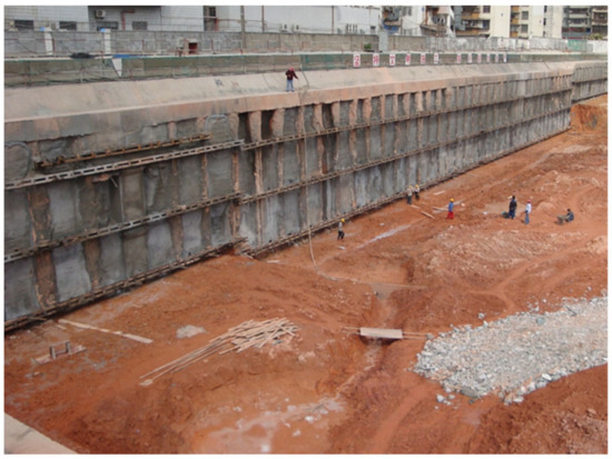
Figure 1.
Foundation pit site in Shenzhen, China.
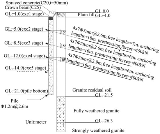
Figure 2.
The sectional view of the deep excavation.

Table 1.
Construction process information.
2.2. Soil Constitutive Model and Support Structure Parameters
- (1)
- The built-in plastic hardening (PH) model in FLAC3D is selected for the soil constitutive models [22]. The model is similar to the hardening soil model in the Plaxis software(version: 3D−2013). It can consider the hyperbolic stress–strain relationship during the triaxial shear phase, plastic strain in mobilizing friction, stress-dependent elastic stiffness, plastic strain generated during the initial compression phase, elastic unloading/reloading behavior, the stress effect considering the preconsolidation strength, and the Mohr–Coulomb failure criterion. For a detailed description of the theoretical model, please see the literature [23]. In general, the model can capture the deformation behavior in foundation pit excavation well [24,25].
For any type of soil layer, the model contains 11 parameters: fundamental parameters, including the soil weight, Poisson’s ratio un/reloading, and Earth pressure coefficient at rest; Mohr–Coulomb strength parameters, including the cohesion, friction angle, and dilatancy angle; stiffness parameters, including the primary loading stiffness (reference), oedometric stiffness (reference), and un/reloading stiffness (reference); hardening parameters, including the stress dependency index; and the reference pressure (atmospheric pressure). These parameters can be obtained from conventional geotechnical tests and the studies of Qin et al. [26] and Liu et al. [27]. The abbreviated names and values of the variables are shown in Table 2.
Table 2.
Input soil parameters in PH model.
- (2)
- For the pit profile studied in this paper, the support structures include slope spray mixing (strength grade C20), a pile (strength grade C25), a crown beam (strength grade C25), a waist beam (strength grade C25), and an anchor (strength grade Φ). Because these construction materials and support structures are produced according to normative standards, the relevant parameters can be obtained according to the standard. For example, C20 represents the standard value of concrete’s compressive strength, which is 20 MPa, and the corresponding elasticity modulus is 25,500 Mpa. These parameters are given directly in Table 3.
Table 3. Supporting structure parameters of foundation pit.
2.3. Model Assumptions, Element Mesh, and Boundary Conditions
The following assumptions are made for efficient model operation.
- In the process of simulation excavation, the site is flat after each excavation, and each over-excavation is 0.5 m. Anchor construction and the application of prestressing are completed instantly, and there is no loss of prestress.
- Since the time for excavation is relatively short, the consolidation analysis is ignored [6].
- Slope spray mixing is considered by the shell element, the anchors are considered by cable elements, and piles are considered by equivalent solid elements, pile elements, and liner elements, respectively, based on different methods of pile equivalent calculation. Crown beams are considered by solid elements and beam elements, and waist beams are divided into two cases considering waist beams (which are considered by beam elements) and without waist beams. For the pile model, more details are shown in Section 2.5.
Based on the typical profile and bolt spacing, the positions of the first two anchor points along the outer extension direction of the vertical profile are indicated by black triangles (Figure 3b), and the third layer of anchors is a black rectangular box. Considering the geometric spacing of the pile anchors and the grid quality, the model is 7.8 m long in the direction of extension outside the vertical profile. It is divided into 12 equally spaced grids, with spacing of 0.65 m each. This division allows for the spatial location in the anchor head to be coupled to the mesh nodes, in order to characterize the stiffening effect during the actual construction (Figure 3a). The soil mesh near the pile body is locally refined to ensure that it will not affect the accuracy of the calculation results, while reducing the calculation time, and this operation is generally recognized by related scholars [28,29].
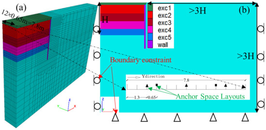
Figure 3.
View of numerical model: (a) 3D view; (b) plane view.
Horizontal motion is constrained at the lateral boundary, while both horizontal and vertical motions are constrained at the bottom boundary (Figure 3b). In addition, the distance between the pile and the outer boundary of the mesh is ensured to be larger than three times the final excavation depth, to minimize the boundary effect [6].
2.4. Modeling of Construction Procedure in FLAC3D
The excavation and support stages of the foundation pit in FLAC3D are in accordance with the actual construction stages, which are shown in Table 1. Specifically, the initial stress field is obtained by applying the K0 gravity field in the FLAC3D model through the elastic solution method, followed by assigning the PH model to the soil body, and then solving the model in order to obtain the stress field under the real soil mechanical parameter conditions. The realization of the pile body is described in detail in Section 2.5. When the soil is dug out, the NULL model is applied in FLAC3D [22]. The prestressing in the anchor is applied by applying the command “apply tension value” to the free section of the anchor. The convergence criterion in the excavation phase is based on the system unbalance force ratio of less than 1× 10⁻⁵.
2.5. Pile Equivalent Calculation Methods
According to the previous research results of scholars, four types of pile equivalent calculation methods are considered in this paper, including equivalent solid elements without the interface (Figure 4a), equivalent solid elements with the interface (Figure 4b), one-dimensional structural elements (Figure 4c), and two-dimensional plate elements (Figure 4d), respectively.
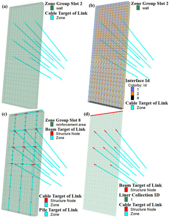
Figure 4.
Support structure schematic diagram for four modes: (a) Mode 1; (b) Mode 2; (c) Mode 3; (d) Mode 4.
- (1)
- Equivalent solid elements without interface (Mode 1)
For Mode 1 (Figure 4a), according to Equation (1), based on the geometric parameters of the piles shown in Figure 2, the equivalent thickness h is 0.77 m, which is simulated by solid elements. No interface elements are used at the soil–pile interface, which means that the soil–pile interface displacement is continuous [30]. A linear–elastic constitutive model is adopted for the solid elements, and the crown beam is considered by solid elements and given the same stiffness parameter values as the solid elements. Without the setting of the waist beam, the anchor head nodes are in rigid contact at the intersection with the solid elements.
- (2)
- Equivalent solid elements with interface (Mode 2)
In Mode 2 (Figure 4b), the pile, crown beam, and anchors are considered the same as in Mode 1, but with the addition of a soil–pile interface element. The shear behavior of the soil–pile interface obeys the Mohr–Coulomb criterion. Since there is no interface between the pile and soil in Mode 1, they are considered to be in good contact [21]. For comparison with Mode 1, the interface shear strength parameters of Mode 2 are set as the soil layer parameters using the control variable method. Hence, the interface friction angle is taken as 22° and the cohesion is 25 kPa, which represents the shear strength index in the second layer of soil. For the flat pit, the normal and tangential stiffness of the interface are recommended as in Equation (2) [22].
where Kn and Ks represent the normal and tangential stiffness of the interface element, respectively. K and G are the bulk modulus and shear modulus of the soil layer, which can be calculated by converting the Young’s modulus and Poisson’s ratio; ∆zmin represents the dimension of the grid near the interface element along the direction of the vertical interface element. According to the relevant parameters, the normal and tangential stiffness are taken as 246 MPa. The anchors are moved halfway towards the inside wall in its X-directional horizontal position, compared to Mode 1, in order to prevent the anchors from interfering with the sliding of the interface element on this side of the pit [22].
- (3)
- One-dimensional structural elements (Mode 3)
In Mode 3 (Figure 4c), the pile structure is simulated with one-dimensional structural elements, namely pile elements. To prevent soil flow between piles [18], the area of reinforcement within the pile diameter of 1.2 m is considered (green part of Figure 4c), and the reinforcement area is simulated with a linear–elastic constitutive model, with a deformation parameter three times that of the surrounding soil. The crown beam and waist beam are simulated using beam elements. The beam, anchor, waist beam, and pile structure elements are in rigid contact at the intersection.
- (4)
- Two-dimensional plate elements (Mode 4)
For Mode 4 (Figure 4d), the pile is equivalent to plate elements according to the equal stiffness method. It is simulated with two-dimensional structural elements, namely embedded liner elements, which consider the soil–pile coupling spring effect [22]. The liner thickness and the parameters of the soil–pile interface are set in the same way as in Mode 2. The crown beam is simulated by beam elements, and the waist beam is ignored. The crown beam, anchor, and liner elements are in rigid contact at the intersection.
3. Results
3.1. Foundation Pit Displacement
Since the pit extends along the vertical profile with a 7.8 m length, considering the pile anchor setting and geometric symmetry, the vertical profile at 3.9 m in the Y direction is selected to extract the displacement for analysis.
3.1.1. Comparison Analysis of Wall Displacement for Four Simulation Methods
Figure 5a–e show the lateral displacement of the pile wall under different excavation stages. It can be seen that when the excavation depth is relatively small, the difference among the results of the four modes is not significant (Figure 5a). When the excavation depth is deeper, only the lateral displacement of Mode 2 increases slowly, while that in the other three modes increases rapidly (Figure 5b,c). At the end of the excavation, the lateral displacement at the wall top of Mode 1 reaches 1.75 times that of Mode 2. Meanwhile, the displacement distribution curves of Mode 3 and Mode 4 are relatively similar, and their lateral displacement at the top of the wall is two times that of Mode 2 (Figure 5e).
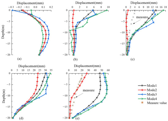
Figure 5.
Comparison analysis of wall lateral displacement under various excavation stages for four modes: (a) 1st excavation stage; (b) 2nd excavation stage; (c) 3rd excavation stage; (d) 4th excavation stage;(e) 5th excavation stage.
3.1.2. Comparison Analysis of Ground Surface Displacement for Four Simulation Methods
Figure 6a–e show the ground surface displacement for the four simulation methods under different excavation stages. Except for Mode 2, the ground settlement tank is essentially the same in all simulation methods during the different excavation stages. In addition, the ground surface settlement distributions of the four simulation methods under various excavation stages show similar characteristics to the lateral displacement. This means that there is good agreement between the lateral displacement and the ground surface settlement performance for the same pile equivalent calculation method. The details of these values will be discussed later in Section 4.1.
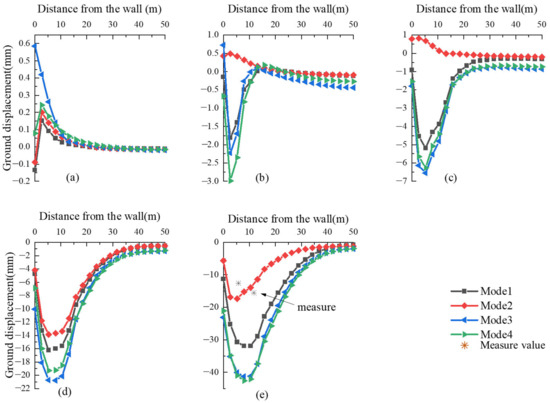
Figure 6.
Comparison analysis of ground displacement under various excavation stages for four modes: (a) 1st excavation stage; (b) 2nd excavation stage; (c) 3rd excavation stage; (d) 4th excavation stage;(e) 5th excavation stage.
3.1.3. Comparison Analysis of Measurement Result and Numerical Result
3.2. Soil Stress
3.2.1. Comparison Analysis of Soil Special Point Stress Paths for Four Simulation Methods
Soil special points’ stress paths may provide useful explanations for changes in soil stress caused by pit excavation [24,31].
In this paper, five representative special points near the wall are selected. The analysis of the stress paths under different pile simulation methods is carried out (the locations of points A, B, C, D, and E are shown in Figure 7a, where the light blue figure represents a schematic diagram of the pit at the end of the excavation stage). Points A and B are located near the bottom of the pile (approximately 17.6 m from the top). Point A is located at the front side of the pile, while point B is at the back side. Point C is located near the upper part of the back side of the pile (approximately 2.3 m from the top). Point D is located in the middle and upper part of the back side of the pile (approximately 5.8 m from the top). Point E is located at the back side of the pile, specifically at the end of excavation (around 13.9 m from the top). Respectively, the Arabic numbers 1, 2, 3 … 6 represent the stages of the initial stress field, i.e., 1st excavation, 2nd excavation … 5th excavation. Since all five special points are located within the second layer of soil, they share the same Kf and K0 lines, where the s-t rectangular coordinate system is adopted as the stress path coordinate system. s, t are recommended as in Equation (3).
where σ1 and σ3 are the first principal stress and the third principal stress, respectively. These values can be programmatically extracted using the FISH language in FLAC3D.
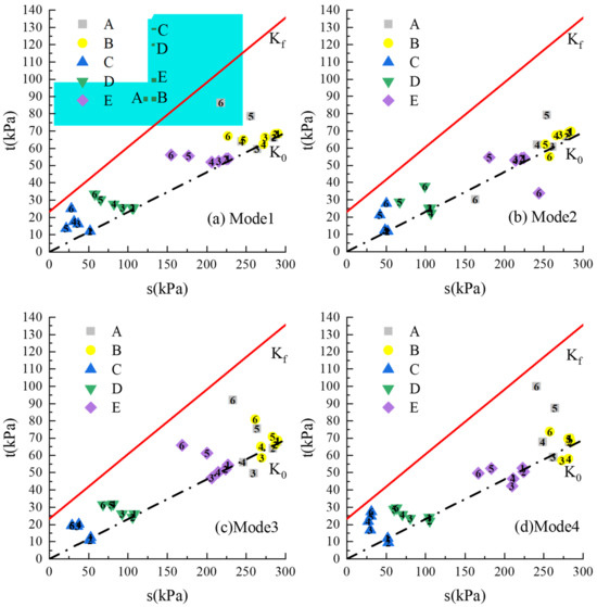
Figure 7.
Comparison of stress paths of special points for four modes under various excavation stages (the Arabic numbers 1, 2, 3 … 6 represent the initial stress field stage, 1st excavation, 2nd excavation … 5th excavation. K0 represents static earth pressure line, Kf represents the breaking line).
Figure 7 shows a comparison of the stress paths at the special points for the four modes under various excavation stages. In the initial stress field stage, the s-t values for these five special points are all located at the K0 line for the four different simulations, which indirectly indicates the accuracy of the model simulation in the initial stress field. As for Mode 1, Mode 3, and Mode 4 in relation to points A and B, as the excavation depth increases, point A, being at the bottom of the excavation area, experiences a more intense stress unloading level compared to point B, resulting in a smaller mean stress at point A and a greater shift in its coordinates towards the left (Figure 7a,c,d). At the same time, because the horizontal stress unloading level at point A is lower than the vertical stress unloading level, its deviator stress becomes larger. As for points C, D, and E, which are located at the back side of the pile, their stress paths are all unloaded strongly horizontally, i.e., the minimum principal stress decreases continuously. From Figure 7a,c,d, it can be found that as the excavation depth increases, the coordinates of these three points shift to the left and steadily move from the initial K0 line to the Kf line.
For Mode 2, it can be found from Figure 7b that the trend of the stress paths at these five special points during the first four excavation stages is similar to that in the other three modes. At the end of the excavation, the mean stress at point A decreases significantly compared to that of the other three modes, dropping from 250 kPa to nearly 160 kPa. The decrease in shear stress causes it to fall below the K0 line. On the other hand, the mean stress at point B slightly increases and also moves below the K0 line. Meanwhile, the mean stress at points C and D increases. The mean stress at point E increases significantly, from 175 kPa in the previous stage to 250 kPa; the reasons for these results will be discussed later in Section 4.2.
3.2.2. Comparison Analysis of Soil Plastic Zone for Four Simulation Methods
Plastic zone statistics are generally used as a validation tool to evaluate the stability of slopes and tunnels [32,33,34,35,36]. They are introduced in the comparison evaluation for the four pile equivalent calculation methods, considering two yield properties, tension and shear yield. There are two methods of calculating the yield zone in FLAC3D. The first method considers the soil zone to have yielded when more than 50% of its volume in a specific grid element has yielded. The second method considers the soil zone to have yielded when any volume of the soil zone has yielded [22]. The first method is adopted for calculation. The shear yield percentage is defined as the ratio of the soil volume that generates shear yield to the total volume of the soil zone for a certain excavation stage, considering the cumulative value of the previous excavation stage. The definition of the tensile yield percentage is similar to that of the shear yield percentage. The above values can be obtained by FISH programming.
As the excavation depth increases, the magnitudes and percentages of shear yield volume resulting from the four modes are as follows: Mode 3 > Mode 1 > Mode 4 > Mode 2 (Figure 8). Meanwhile, the magnitudes and percentages of tension yield volume resulting from the four modes are as follows: Mode 4 > Mode 3 > Mode 1 > Mode 2 (Figure 9). The plastic zone in Mode 2 is at a minimum.
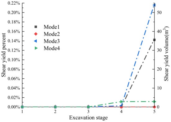
Figure 8.
Comparison of the shear yield percentage and shear yield volume for four modes under various excavation stages.
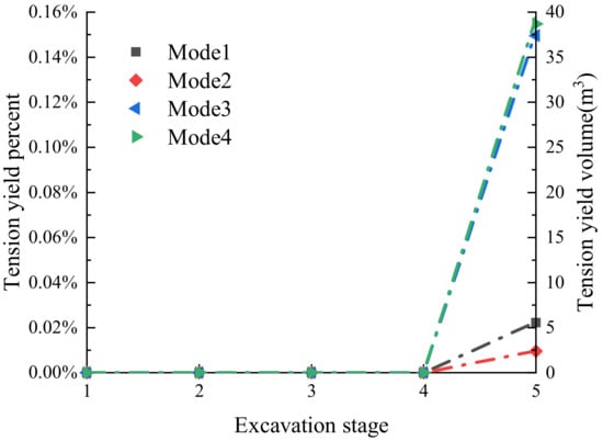
Figure 9.
Comparison of the tension yield percentage and tension yield volume for four modes under various excavation stages.
4. Discussion
4.1. Comparison of Simulation Results with Empirical Methods
Clough and O’Rourke [37] indicated that δehm/He (δehm represents the maximum lateral displacement of the wall in the final excavation stage; He represents the final excavation depth) was around 0.2%, with the upper bound of 0.5%. The results of the four simulation methods in the final excavation stage (Figure 10) are close to 0.4% for Mode 3 and Mode 4, while that for Mode 2 is below approximately 0.2%, and the result from Mode 1 is at an intermediate level among them. In this paper, we extend the study to each excavation stage, (δhm represents the maximum lateral displacement under various excavation stages; H represents the depth of the excavation corresponding to the excavation stage). It can be found that the results of Mode 1, Mode 3, and Mode 4 remain relatively consistent until the final excavation stage, around 0.2%. Meanwhile, that for Mode 2 increases from 0.0% to 0.2% with the increase in the excavation depth.
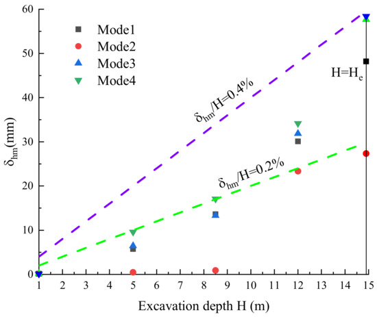
Figure 10.
Comparison of simulation results and empirical methods with maximum lateral displacement under various excavation stages.
Similarly, Clough and O’Rourke [37] indicated that δevm/He (δevm represents the maximum ground surface displacement in the final excavation stage) was around 0.15%, with an upper bound of 0.5%. The results of the four simulation methods in the final excavation stage (Figure 11) are close to 0.3% for Mode 3 and Mode 4, while that for Mode 2 is below approximately 0.2%, and the result from Mode 1 is at an intermediate level among them. Similarly, we extend the study to each excavation stage (δevm represents the maximum ground surface settlement under various excavation stages). As the excavation deepens, the results of Mode 1, Mode 3, and Mode 4 remain consistent until the final excavation stage, with an increase from 0.05% to 0.15%, while that for Mode 2 increases from 0.0% to 0.15%.
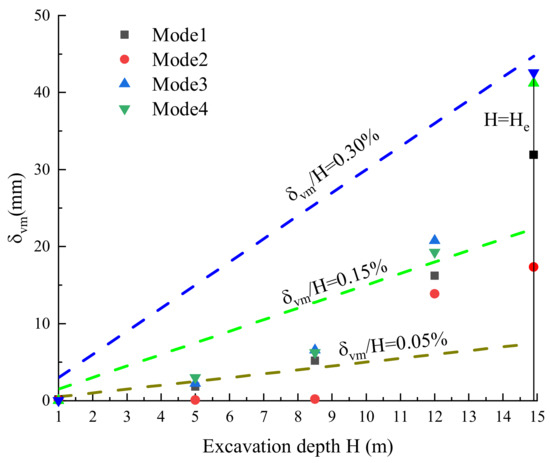
Figure 11.
Comparison of simulation results and empirical methods with maximum settlement under various excavation stages.
As shown in Figure 12, the maximum lateral displacement calculated using the same pile equivalent calculation method corresponds well with the ground settlement [38]. The relationship between the maximum lateral displacement and ground settlement generated by the four modes can be described by the same linear equation.
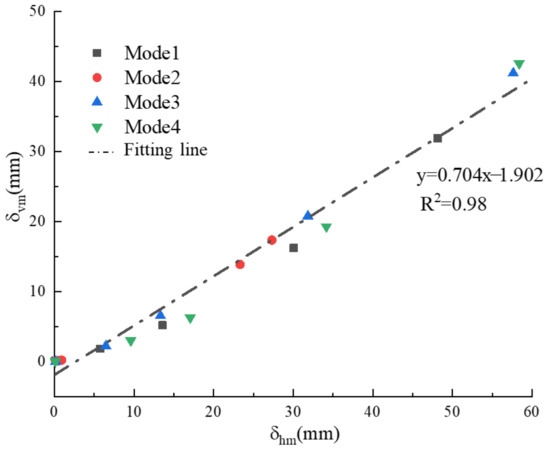
Figure 12.
Relationship between maximum lateral displacement and maximum ground surface settlement in four modes.
4.2. Control Mechanism of Soil Stress by Four Pile Equivalent Calculation Methods
Figure 13 shows the stress tensor and the stress diagram in the XX direction for the four pile simulation methods at the end of the excavation, and the cross-section selected for analysis is the same as in Section 3.1.
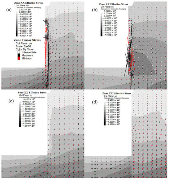
Figure 13.
Comparison of stress tensor and stress diagram in XX direction for four modes at the 5th excavation stage: (a) Mode 1; (b) Mode 2; (c) Mode 3; (d) Mode 4.
The piles in Mode 1 (Figure 13a) and Mode 2 (Figure 13b) are simulated using equivalent solid elements. Due to the large differences in the stiffness parameters between the equivalent solid elements and the soil (Table 2 and Table 3), the equivalent solid elements’ deformation is very small, and the stress discharge of the equivalent solid elements is less than that of the nearby soil, so the solid elements’ stress tensor changes drastically, which is also confirmed by the fact that there is no excessive change in the stress of the reinforcement area in Mode 3 (Figure 13c). Moreover, the stress concentration is observed at two special locations in Mode 1, respectively, at the head of the first layer anchor and the second layer anchor; since the anchor head of Mode 1 is in rigid contact with the equivalent solid elements, the displacement of both is synergistic at this location. The reason that stress concentration occurs only at the two locations is the rapid increase in the anchor axial force in these two layers during this excavation stage (Figure 14).
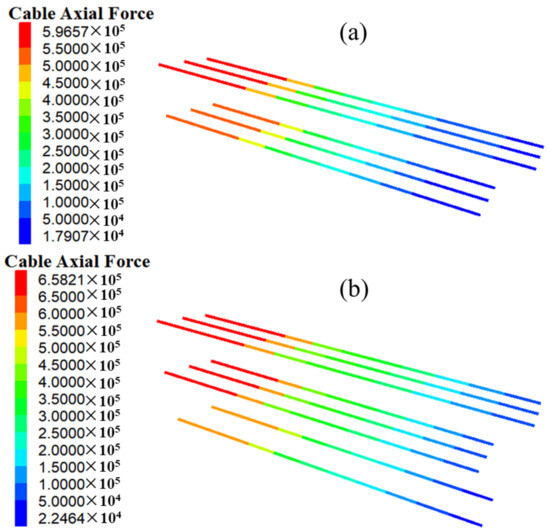
Figure 14.
Comparison of cable axial force for Mode 1: (a) 4th excavation stage; (b) 5th excavation stage.
The maximum horizontal stresses of Mode 1, Mode 3, and Mode 4 are the same; all of them are less than 500 kPa. As for Mode 2, the stress concentration pattern shows a block distribution. The maximum horizontal compressive stress reaches 720 kPa, which is 1.44 times that of the other three modes, located at the side behind the wall at the bottom of the excavation face. As point E is located in an area of intense stress concentration, the point E stress path is different from that of the other three modes (Figure 7b). By checking the interface element (Figure 15), it is found that both the normal stresses and shear stress are maximum in this part of the area. Therefore, it is suggested that the interface element is responsible for the stress concentration in this area.
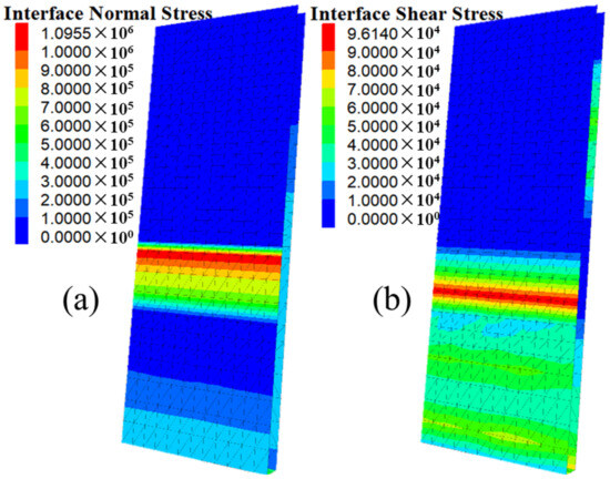
Figure 15.
Normal and tangential stresses of the interface element at the 5th excavation stage for Mode 2: (a) normal stresses of the interface element; (b) tangential stresses of the interface element.
As for Mode 3 and Mode 4, since the anchor heads are only rigidly connected to the structural elements, and there are no equivalent solid elements with a significant difference in stiffness compared to the adjacent soil, there is no stress concentration. Hence, the stress distribution and stress tensor distribution are essentially the same for both modes. Moreover, since the magnitudes of the stress tensor near the pile side in Mode 3 and Mode 4 are smaller than those in Mode 1and Mode 2, the level of stress unloading in Mode 3 and Mode 4 is greater, resulting in greater deformation. This is also evidenced by the larger lateral displacement and ground displacement in Mode 3 and Mode 4 (Figure 5e and Figure 6e).
5. Conclusions and Recommendations for Further Research
This study focuses on analyzing the differential effects and intrinsic mechanisms brought about by different pile body equivalent calculation methods in pile–anchor foundation pits’ numerical simulation. The investigation is conducted from the perspectives of soil displacement and stress, stress paths at special points, and plastic zones. The main findings are as follows.
- (1)
- With the increase in excavation depth, the displacement results produced by different pile equivalent calculation methods are significantly different, and the pile simulated with solid units has smaller horizontal displacement on the pile side and surface settlement. The displacement distribution characteristics under the simulation conditions of a one-dimensional structural unit and two-dimensional plate unit are basically the same, and the displacements are larger. In this study, the results of the solid unit with an interface unit are closer to the measured data.
- (2)
- The linear relationship between the maximum surface settlement and the maximum horizontal displacement of the pile side corresponding to the four simulation methods at each excavation stage can be characterized by the following equation: y = 0.704x − 1.902 (R2 = 0.98). Its pile-side displacement/excavation depth (δhm/H) is clustered around 0.2% and its surface settlement/excavation depth (δvm/H) is clustered around 0.15%.
- (3)
- As the excavation proceeds, the soil units close to the pile side move from the K0 line to the damage line, the Kf line, which is attributed to the effect of horizontal unloading caused by the foundation pit’s excavation. In solid unit simulation conditions, the stress results show that stress concentration will be formed at a certain part of the pile side, which leads to a significant change in the stress paths near the pile side.
- (4)
- Among the four simulation methods, the solid unit with interface unit simulation method results in the lowest percentage of shear yield and tensile yield in the foundation soil, which may be attributed to the combination of the interface unit and the solid unit.
Overall, the results of different pile body equivalent calculation approaches are significantly different. This study provides valuable insights into the equivalent calculation methods for pile bodies in numerical simulations. Of course, there are still some limitations in the research work. These four simulation equivalent calculation methods should be applied to more engineering cases in the future and compared with the relevant site monitoring data to determine which model is suitable for specific engineering construction conditions.
Author Contributions
Conceptualization, X.L.; methodology, X.L. and H.L.; software, X.L. and H.L.; data curation, X.L. and D.W.; writing—original draft preparation, X.L.; writing—review and editing, C.W. and D.W.; project administration, C.W.; funding acquisition, C.W. All authors have read and agreed to the published version of the manuscript.
Funding
This research was funded by the National Natural Science Foundation of China (Grant No. 41972267).
Institutional Review Board Statement
Not applicable.
Informed Consent Statement
Not applicable.
Data Availability Statement
Data may be requested from the corresponding author.
Conflicts of Interest
The authors declare no conflict of interest.
References
- Rouainia, M.; Elia, G.; Panayides, S.; Scott, P. Nonlinear Finite-Element Prediction of the Performance of a Deep Excavation in Boston Blue Clay. J. Geotech. Geoenviron. Eng. 2017, 143, 04017005. [Google Scholar] [CrossRef]
- Orazalin, Z.Y.; Whittle, A.J.; Olsen, M.B. Three-Dimensional Analyses of Excavation Support System for the Stata Center Basement on the MIT Campus. J. Geotech. Geoenviron. Eng. 2015, 141, 05015001. [Google Scholar] [CrossRef]
- Chen, A.; Wang, Q.; Chen, Z.; Chen, J.; Chen, Z.; Yang, J. Investigating pile anchor support system for deep foundation pit in a congested area of Changchun. Bull. Eng. Geol. Environ. 2021, 80, 1125–1136. [Google Scholar] [CrossRef]
- Lan, B.; Wang, Y.; Wang, W. Review of the Double-Row Pile Supporting Structure and Its Force and Deformation Characteristics. Appl. Sci. 2023, 13, 7715. [Google Scholar] [CrossRef]
- Yin, Q.; Fu, H.; Zhou, Y. Spatial Deformation Calculation and Parameter Analysis of Pile–Anchor Retaining Structure. Appl. Sci. 2023, 13, 6637. [Google Scholar] [CrossRef]
- Lim, A.; Ou, C.Y.; Hsieh, P.G. An innovative earth retaining supported system for deep excavation. Comput. Geotech. 2019, 114, 103135. [Google Scholar] [CrossRef]
- Chen, S.L.; Chang, S.W.; Qiu, Z.Y.; Tang, C.W.; Zhang, X.L.; Chen, Y. Numerical Model for Rectangular Pedestrian Underpass Excavations with Pipe-Roof Preconstruction Method: A Case Study. Appl. Sci. 2023, 13, 5952. [Google Scholar] [CrossRef]
- Zhang, W.; Li, Y.; Goh, A.T.C.; Zhang, R. Numerical study of the performance of jet grout piles for braced excavations in soft clay. Comput. Geotech. 2020, 124, 103631. [Google Scholar] [CrossRef]
- Yuan, X.Y.; Chen, L.Z.; Deng, J.L. Calculation of displacements and internal forces of anchored retaining piles. PLoS ONE 2020, 15, e0243659. [Google Scholar] [CrossRef]
- Deshmukh, V.B.; Dewaikar, D.M.; Choudhury, D. Computations of uplift capacity of pile anchors in cohesionless soil. Acta Geotech. 2010, 5, 87–94. [Google Scholar] [CrossRef]
- Liu, Y.; Wang, C.M.; Liu, X.Y.; Gao, R.Y.; Li, B.L.; Khan, K.U.J. Determination of Embedded Depth of Soldier Piles in Pile-Anchor Supporting System in Granite Residual Soil Area. Geofluids 2021, 2021, 5518233. [Google Scholar] [CrossRef]
- Schweiger, H.F.; Tschuchnigg, F. A numerical study on undrained passive earth pressure. Comput. Geotech. 2021, 140, 104441. [Google Scholar] [CrossRef]
- Peng, Y. Construction Design of Pile Anchor Support in Deep Foundation Pit Excavation. Int. J. Mutiphysics 2021, 15, 19–28. [Google Scholar]
- Li, S.Z.; Ren, F.; Sheng, G.L.; Zhao, W.P. Three-dimensional numerical analysis of deformation of various combined support forms. In Proceedings of the 4th International Conference on Applied Materials and Manufacturing Technology 2018, Nanchang, China, 25–27 May 2018; IOP Publishing Ltd.: Bristol, UK. [Google Scholar]
- Shao, Y.; Zhu, J.J.; Liu, X.L. Analysis of Influencing Factors of Supporting Effect for Pile-Anchor in Soft Soil Foundation. J. Geotech. Eng. 2016, 21, 5229–5245. [Google Scholar]
- Dieterman, H.; Metrikine, A. The equivalent stiffness of a half-space interacting with a beam. Critical velocities of a moving load along the beam. Eur. J. Mech. Ser. A Solids 1996, 15, 67–90. [Google Scholar]
- Bhattacharya, S.; Adhikari, S.; Alexander, N.A. A simplified method for unified buckling and free vibration analysis of pile-supported structures in seismically liquefiable soils. Soil Dyn. Earthq. Eng. 2009, 29, 1220–1235. [Google Scholar] [CrossRef]
- Zheng, G.; Zhu, X.; Cheng, X.; Lei, Y.; Wang, R.; Zhao, J.; Yi, F. Study on the control theory and design method of progressive collapse in excavations retained by cantilever piles. Chin. J. Geotech. Eng. 2021, 43, 981–990. (In Chinese) [Google Scholar]
- Wang, S.; Li, Q.; Dong, J.; Wang, J.; Wang, M. Comparative investigation on deformation monitoring and numerical simulation of the deepest excavation in Beijing. Bull. Eng. Geol. Environ. 2021, 80, 1233–1247. [Google Scholar] [CrossRef]
- Wang, G.X.; Sun, X.L.; Zhao, W.P. Influence of Excavation of Complex Foundation Pit on Surrounding Environment. In Proceedings of the 4th International Conference on Applied Materials and Manufacturing Technology 2018, Nanchang, China, 25–27 May 2018; IOP Publishing Ltd.: Bristol, UK. [Google Scholar]
- Liu, L.L.; Wu, R.G.; Congress, S.S.C.; Du, Q.W.; Cai, G.J.; Li, Z. Design optimization of the soil nail wall-retaining pile-anchor cable supporting system in a large-scale deep foundation pit. Acta Geotech. 2021, 16, 2251–2274. [Google Scholar] [CrossRef]
- Itasca. FLAC3D 6.0 Document; Itasca Consulting Group: Minneapolis, MN, USA, 2018. [Google Scholar]
- Liu, H.; Han, J.; Parsons, R.L. Numerical analysis of geosynthetics to mitigate seasonal temperature change-induced problems for integral bridge abutment. Acta Geotech. 2023, 18, 673–693. [Google Scholar] [CrossRef]
- Ayizula, A.; Liu, J. Inverse analysis on compressibility of toronto clays. Soils Found. 2023, 63, 101280. [Google Scholar] [CrossRef]
- Wu, Y.B.; Ye, J.B.; Ge, H.B.; Liu, G.Q.; Liu, H.W. Numerical investigation of dual-row batter pile wall in deep excavation. Mech. Adv. Mater. Struct. 2021, 15, 5793–5807. [Google Scholar] [CrossRef]
- Qin, S.W.; Miao, Q.; Zhang, L.S.; Zhang, Y.Q.; Cheng, Q.S. Finite element analysis on influence of excavation and support removal of foundation pit to surrounding environment. J. Eng. Geol. 2020, 28, 1106–1115. (In Chinese) [Google Scholar]
- Liu, Z.; Li, Z.C.; Liu, G.N. Study on parameters determination of modified mohr-coulomb model for granite residual soil in deep foundation pit simulation analysis. Railw. Eng. 2017, 3, 89–92. (In Chinese) [Google Scholar]
- Al-Maadheedi, M.A.; Dekker, M.J. Numerical modelling of sand plug formation during punch-through of a spudcan footing. Ocean Eng. 2023, 284, 115198. [Google Scholar] [CrossRef]
- Tan, J.P.S.; Goh, S.H.; Tan, S.A. Numerical Analysis of a Jacked-In Pile Installation in Clay. Int. J. Geomech. 2023, 23, 04023061. [Google Scholar] [CrossRef]
- Ng, C.W.W.; Zheng, G.; Ni, J.J.; Zhou, C. Use of unsaturated small-strain soil stiffness to the design of wall deflection and ground movement adjacent to deep excavation. Comput. Geotech. 2020, 119, 103375. [Google Scholar] [CrossRef]
- Ignat, R.; Baker, S.; Karstunen, M.; Liedberg, S.; Larsson, S. Numerical analyses of an experimental excavation supported by panels of lime-cement columns. Comput. Geotech. 2020, 118, 16. [Google Scholar] [CrossRef]
- Wang, T.; Wu, H.G.; Li, Y.; Gui, H.Z.; Zhou, Y.; Chen, M.; Xiao, X.; Zhou, W.B.; Zhao, X.Y. Stability analysis of the slope around flood discharge tunnel under inner water exosmosis at Yangqu hydropower station. Comput. Geotech. 2013, 51, 1–11. [Google Scholar] [CrossRef]
- Darvishi, A.; Ataei, M.; Rafiee, R. Investigating the effect of simultaneous extraction of two longwall panels on a maingate gateroad stability using numerical modeling. Int. J. Rock Mech. Min. Sci. 2020, 126, 104172. [Google Scholar] [CrossRef]
- Yi, K.; Kang, H.P.; Ju, W.J.; Liu, Y.D.; Lu, Z.G. Synergistic effect of strain softening and dilatancy in deep tunnel analysis. Tunn. Undergr. Space Technol. 2020, 97, 12. [Google Scholar] [CrossRef]
- Zhang, Y.G.; Zhang, Z.; Xue, S.; Wang, R.J.; Xiao, M. Stability analysis of a typical landslide mass in the Three Gorges Reservoir under varying reservoir water levels. Environ. Earth Sci. 2020, 79, 42. [Google Scholar] [CrossRef]
- Fan, Y.; Zheng, J.W.; Cui, X.Z.; Leng, Z.D.; Wang, F.; Lv, C.C. Damage zones induced by in situ stress unloading during excavation of diversion tunnels for the Jinping II hydropower project. Bull. Eng. Geol. Environ. 2021, 80, 4689–4715. [Google Scholar] [CrossRef]
- Clough, G.W.; O’Rourke, T.D. Construction Induced Movements of Insitu Walls. Geotech. Spec. Publ. 1990, 25, 439–470. [Google Scholar]
- Hsieh, P.-G.; Ou, C.-Y. Shape of ground surface settlement profiles caused by excavation. Can. Geotech. J. 1998, 35, 1004–1017. [Google Scholar] [CrossRef]
Disclaimer/Publisher’s Note: The statements, opinions and data contained in all publications are solely those of the individual author(s) and contributor(s) and not of MDPI and/or the editor(s). MDPI and/or the editor(s) disclaim responsibility for any injury to people or property resulting from any ideas, methods, instructions or products referred to in the content. |
© 2023 by the authors. Licensee MDPI, Basel, Switzerland. This article is an open access article distributed under the terms and conditions of the Creative Commons Attribution (CC BY) license (https://creativecommons.org/licenses/by/4.0/).