Article

Analyzing Physics-Inspired Metaheuristic Algorithms in Feature Selection with K-Nearest-Neighbor

1
School of Computer Science and Engineering, Vellore Institute of Technology, Chennai 600027, India
2
Department of Machining, Assembly and Engineering Metrology, Faculty of Mechanical Engineering, VSB-Technical University of Ostrava, 17. Listopadu 2172/15, 708 00 Ostrava, Czech Republic
3
Department of Mechanical Engineering, Vel Tech Rangarajan Dr. Sagunthala R&D Institute of Science and Technology, Avadi 600062, India
*
Author to whom correspondence should be addressed.
Appl. Sci. 2023, 13(2), 906; https://doi.org/10.3390/app13020906
Submission received: 12 September 2022 / Revised: 30 December 2022 / Accepted: 6 January 2023 / Published: 9 January 2023
(This article belongs to the Section Computing and Artificial Intelligence)

Abstract

:
In recent years, feature selection has emerged as a major challenge in machine learning. In this paper, considering the promising performance of metaheuristics on different types of applications, six physics-inspired metaphor algorithms are employed for this problem. To evaluate the capability of dimensionality reduction in these algorithms, six diverse-natured datasets are used. The performance is compared in terms of the average number of features selected (AFS), accuracy, fitness, convergence capabilities, and computational cost. It is found through experiments that the accuracy and fitness of the Equilibrium Optimizer (EO) are comparatively better than the others. Finally, the average rank from the perspective of average fitness, average accuracy, and AFS shows that EO outperforms all other algorithms.

1. Introduction

Data mining is the process of finding meaningful information or extracting knowledge from large amounts of data. Data mining has the challenging problem of dealing with huge data dimensions. When working with data that has a large number of dimensions, even the advantages of technology can be a hassle [1]. The data-mining process may suffer due to a huge number of dimensions. It may also require a lot of computing time and space. Traditional machine-learning (ML) methods cannot handle these huge datasets [2]. The dataset is made up of several samples that collectively give information about a specific case of the problem. Each sample has a variety of attributes or features. The dataset may have several superfluous or duplicate attributes, in addition to its huge dimensionality. The model may be complex, and the dataset may include a substantial amount of noise. The best subset of the useful features that will contribute to the output is chosen via a pre-processing technique called feature selection (FS) [2]. FS can reduce the training time as well as the huge number of dimensions in the data. Moreover, the model’s accuracy is enhanced in addition to the simplification of the model and the best utilization of computing resources [3].
The two main FS approaches are wrapper methods and filter methods. The major drawback of the filter methods is that they work independently of the ML classifiers and do not take any input from them [4]. Meanwhile, the wrapper method uses the classifier directly and picks the features using an optimization algorithm [5]. Optimization algorithms provide the advantage of choosing an optimal or nearly optimal subset of features in a reasonable amount of time as opposed to the conventional exhaustive search. An exhaustive search becomes impractical, because it finds the solution by creating all feasible feature subsets ( 2 m different solutions for m features) [6]. In the literature, optimization algorithms are categorized into several groups, such as evolution-based algorithms, swarm-based algorithms, human behavior-inspired algorithms, physics-inspired algorithms, etc. [7]. Swarm-based algorithms mimic the collective but decentralized intelligence of living creatures, such as birds [8], wolves [9], whales [10], bacteria [11], etc. Evolutionary algorithms mimic the emergence of the fittest and healthiest individuals over generations. A few examples are the Genetic Algorithm (GA) [12], Differential Evolution (DE) [13], Biogeography-Based Optimization (BBO) [14], etc. Human behavior-inspired algorithms mimic the collective intelligent behavior of human beings in different real-life situations, such as politics [15], sports [16], corporations [7], etc. Finally, physics-based algorithms are inspired by the laws of nature, such as the gravitational law [17], black holes [18], galaxies [19], etc.
In recent years, metaphor-based algorithms have extensively been used to solve FS problems from different domains. Examples include feature selection using Particle Swarm Optimization (PSO) for document clustering [20], the use of a real-valued Grasshopper Optimization Algorithm (GOA) for feature selection [21], hybridization of the Whale Optimization Algorithm (WOA) and Simulated Annealing (SA) for the feature selection problem [22], feature selection for intrusion detection in wireless mesh networks incorporating genetic operators in WOA [23], the incorporation of levy flight and opposition-based learning in chaotic Cuckoo Search (CS) for feature selection [24], feature selection using Moth Flame Optimization (MFO) [25], feature selection using the Firefly Algorithm (FA) [26], the hybridization of SA with Harris Hawk Optimization (HHO) for the feature selection problem [27] and feature selection using binary Teaching–Learning-Based Optimization (TLBO).
According to the No-Free-Lunch (NFL) theorem [28], no single optimization algorithm is capable of solving every optimization problem by outperforming all other optimization techniques. Because of this, one optimizer can perform better than the others on some problems, but not on all of them. Hence, it is crucial to compare several optimization algorithms on a variety of datasets to find the optimum solution to the feature selection problem. Since there are hundreds of optimization algorithms in the literature, in this study, a few well-known and highly cited physics-inspired algorithms are chosen for this purpose. The rationale is to carry out a comparison of the various metaphors drawn from physics and evaluate their effectiveness. To evaluate the performance of these algorithms, six small-to-large-sized classification datasets are used. The accuracy, convergence, and average fitness of these algorithms are compared. This paper has the following contributions:
  • The main novelty of our paper lies in its comparative analysis of six well-cited physics-inspired metaphor algorithms for the problem of feature selection.
  • To the best of our knowledge, this is the first time these physics-inspired algorithms have been compared for this specific problem, and our findings provide valuable insights into their performance.
  • Our study also has broader implications for the field of machine learning and data mining, as it helps to shed light on the effectiveness of different optimization algorithms for feature selection.
  • Our work contributes to the growing body of research on metaheuristics and their potential applications in machine learning and data mining, and it highlights the potential value of using physics-inspired optimization algorithms for feature selection.
  • Additionally, our use of variable-sized classification datasets allows us to assess the applicability of these algorithms on a wide range of problems, making our results more generalizable and applicable to practitioners.
Overall, we believe that our paper represents a significant contribution to the field and has the potential to impact the way practitioners approach the problem of feature selection. The rest of the paper is organized as follows. The methodology is discussed in Section 2. Section 3, namely, the Results and Discussion, covers the results and comparative analysis of all six algorithms, and the concluding remarks are given in Section 4.

2. Methodology

2.1. Wrapper Method for Feature Selection

For feature selection, we employed a wrapper method. To accomplish their task, wrapper techniques use a learning algorithm that applies a search strategy to explore the space of feasible feature subsets, ranking them according to the quality of their performance in a specific algorithm. In most cases, wrapper approaches outperform filter methods, since the feature selection process is tailored to the specific classification algorithm being employed. Wrapper methods, on the other hand, are prohibitively time- and resource-intensive for high-dimensional data, since they require evaluating each feature set with the classifier algorithm. Figure 1 depicts the way in which wrapper methods function.
In this paper, K-Nearest Neighbor (k-NN) is used as the evaluator algorithm. The k-NN method uses a set of K neighbors to determine how an object should be categorized. A positive integer value of K is pre-decided before running the algorithm. To classify a record, the Euclidean distances between the unclassified record and the classified records are determined and ranked.

2.2. Fitness Function

The effectiveness of an optimizer is evaluated by its fitness function. The fitness function in feature selection is dependent on the classification error rate and the number of features used for classification. It is deemed to be a good solution if the selected feature subset reduces the classification error rate and the number of features chosen. The following fitness function is used in this paper [29]:
  F i t n e s s = λ γ S ( D ) + ( 1 λ ) | S | | F |
where γ S ( D ) is the classification error computed by the classifier, | S | is the reduced number of features in the new subset, | F | is the total features in the dataset, and λ   ϵ   [ 0 ,   1 ] is a factor corresponding to the importance of the classification performance and length of the reduced subset.

2.3. Physics-Inspired Metaphor Algorithms

In this paper, six well-cited physics-inspired metaphor algorithms are employed to solve the problem of feature selection. In this section, the functioning of these algorithms and their position-updating mechanisms are discussed.

2.3.1. Simulated Annealing

Simulated Annealing is a fundamental nature-inspired algorithm that was proposed in 1983 by Kirkpatrick et al. [30]. The source of inspiration behind this algorithm is the annealing process of metals. The process of annealing, which starts at a very high temperature and progressively cools down, is used to physically harden metals. The algorithm involves three main parameters, including the cooling rate ( c ), the final temperature ( T f ), and the starting temperature ( T 0 ). The starting temperature is kept very high initially, and the cooling rate gradually reduces until it reaches the final temperature. The process is mimicked by randomly generating a candidate solution. The algorithm runs iteratively, and a new solution is generated in the neighborhood of the current solution in each iteration. The fitness of the current and neighbor solutions is compared. If the fitness of the new solution is better, then the position of the current solution is updated. Moreover, the best solution keeps the best position found so far. The terminating condition of the repetitive process is reaching the T f . In each iteration, T is updated as follows:
T = T C ,                                         0 < c < 1
SA is a global optimization algorithm, because it can explore as well as exploit the search space. The exploration is performed by updating the current solution with a worse neighboring solution in early iterations based on the value of T and the worse value of the neighboring solution. The chance of accepting the worse neighbor is computed using the following equation:
exp ( δ T ) r
where exp is the exponential function, δ is equal to the fitness difference of current and neighboring solutions, and r is randomly generated in the range [0, 1].

2.3.2. Gravitational Search Algorithm

This algorithm is inspired by Newton’s law of gravitation and the second law of motion [17]. It treats each candidate solution in the search space as an object whose mass is considered to be its fitness. Heavier objects are considered fitter than lighter objects. The objects are attached to each other with some gravitational force that causes objects to explore the search space. The heaviest object is considered the global best solution. Since the heavier objects attract other objects with more force, the whole population ultimately converges toward the heaviest object, called the global best solution. The algorithm is comprised of a few mathematical equations that are expressed below.
Force calculation: The force from an object j on an object i is calculated using the following equation:
F i j d ( t ) = G ( t ) M p i ( t ) × M a j ( t ) R i j ( t ) + ϵ ( x j d ( t ) x i d ( t ) )
In the above equation, G is the gravitational constant that controls the search accuracy, M p i is the passive gravitational mass of solution i , M a j is the active gravitational mass of solution j , the distance between solution i and solution j is denoted by R i j , x d is the position of a solution in d th dimension, and ϵ is a small constant.
The ultimate force on a solution (mass) is calculated by taking the weighted sum of all the forces on that solution from the k b e s t solutions, which are calculated as follows:
F i d ( t ) = j k b e s t ,   j i r a n d j F i j d ( t )
Acceleration calculation: Once the total force on a solution in a particular dimension d is calculated, the acceleration of the solution in that dimension can be computed using the following equation:
a i d ( t ) = F i d ( t ) M i i ( t )
where M i i is the mass of inertia of solution i.
Velocity calculation: Based on the acceleration, the velocity of a solution can be computed by adding the acceleration to a fraction of the previous velocity of that solution. The equation to compute velocity is given below:
v i d = r a n d i × v i d ( t ) + a i d ( t )
Position updating: To update the position of a solution, the updated velocity is simply added to the old position of the solution, as formulated below:
x i d ( t + 1 ) = x i d ( t ) + v i d ( t + 1 )
Gravitational constant updating: To update G , the following relation is used:
G ( t ) = G 0 exp ( α t t m a x )
where G 0 is the initial gravitational constant, and α is a constant. t and t m a x represent the current and final iteration numbers.

2.3.3. Sine Cosine Algorithm

The Sine Cosine Algorithm (SCA) [31] has a very unique source of inspiration. It utilizes two sine and cosine functions to update the position of solutions when searching the space to find the global optimum. The position-updating model of this algorithm is very simple and is formulated below:
X i t + 1 = { X i t + r 1 × sin ( r 2 ) × | r 3 P i t X i t | , r 4 < 0.5 X i t + r 1 × cos ( r 2 ) × | r 3 P i t X i t | , r 4 0.5
In the above equation, X i denotes a solution in the i th dimension, and P i denotes the global best solution, namely, the destination solution in the paper. The above equation involves a few other variables that are defined below.
r 1 is an adaptive parameter that is linearly reduced with the course of iterations. It starts from a prefixed value and linearly decreases in each iteration. It is computed as follows:
r 1 = α t   α T
where α is constant.
  • r 2 is randomly generated in the range of 0 to 2π.
  • r 3 is also a random number that is generated in the range of 0 to 2.
  • r 4 is also a random number that is generated in the range of 0 to 1, and based on its value, it is decided whether to use the sine function or the cosine function in updating the position of the current solution.
When multiplied by r 1 , the range of values provided by sin( r 2 ) and cos( r 2 ) shifts from [−1, 1] to [−2, 2]. Due to a linear decrease in the values of the parameter r 1 , the range begins at [−2, 2] and linearly declines to [0, 0] during iterations. The position-updating equation of SCA creates two regions around the destination P: an inner region that promotes exploitation and an outer region to promote exploration. The precondition to search the inner region is { 1 < = r 1   X   cos ( r 2 ) < = 1 } or { 1 < = r 1   X   sin ( r 2 ) < = 1 } , and the precondition to search the outer region is { r 1   X   cos ( r 2 ) } , or { r 1   X   sin ( r 2 ) } gives a value greater than 1 or lesser than −1.

2.3.4. Atom Search Optimization

Atom Search Optimization (ASO) [32], which is inspired by molecular dynamics, has shown a tremendous performance on a variety of applications in the literature. Each atom is considered a candidate solution, and the mass is mapped with the fitness in the optimization algorithm, where the higher the mass, the fitter the solution. Every atom in the population pulls or repels other atoms in the search space. The heavier atoms generate more force and pull lighter objects rapidly, and the heavier objects are pulled slowly towards the others due to their mass. The slowly moving atoms create exploitation in the algorithm, because they can search more locally, whereas the rapidly moving atoms allow the algorithm to explore the search space because of longer and quicker jumps. The algorithm starts with random initializations. In every iteration, the atoms move and accelerate, and the location of the atom that has performed the best up to that point is also likewise adjusted. Atomic acceleration is also caused by two other factors: L-J potential and constraint forces. The acceleration helps to update the velocity of the solutions (atoms). Finally, the velocity is added to the previous position to update the current position of the solution. The position-updating mechanism of the algorithm is discussed below.
The population is generated by randomly generating position and velocity vectors for each atom in the population.
X i = [ X i 1 ,   X i 2 ,   ,   X i D ]
V i = [ V i 1 ,   V i 2 ,   ,   V i D ]
The fitness of each solution in the population is computed, and the global best X b e s t is determined.
The mass of each atom is computed using the following equation:
m i = M i j = 1 N M j
where M is computed from the fitness of the current solution, the best solution, and the worst solution.
The value of K is computed, where K denotes the size of the subset of atoms:
K = N ( N 2 ) t T
where N is the size of the population.
The interaction force on an atom is calculated, which is accomplished using the following equation:
F i d = j K r a n d j F i j d
where r a n d j is a random number in the range of [0, 1].
The constraint force is computed using the following equation:
G i d = λ   ( X b e s t d X i d )
where λ is the Langrangian multiplier that is computed as follows:
λ = β   e T 20 t
where β is the multiplier weight.
Once the mass, constraint forces, and interaction forces are computed, the acceleration is computed as follows:
a i d = F i d m i d + G i d m i d
Once the acceleration is computed, the velocity of an atom can be computed as follows:
V i d ( t + 1 ) = r 1 V i d ( t ) + a i d ( t )
Using the updated velocity, the position of a solution is updated as follows:
X i d ( t + 1 ) = X i d ( t ) + V i d ( t + 1 )

2.3.5. Henry Gas Solubility Optimization

Henry Gas Solubility Optimization (HGSO) is inspired by Henry’s gas law [33], which is stated below:
At a constant temperature, the amount of a given gas that dissolves in a given type and volume of liquid is directly proportional to the partial pressure of that gas in equilibrium with that liquid”.
This law can be interpreted as the partial pressure of a gas and the solubility of that gas being directly proportional. If one increases, then the other increases, too. This relation is expressed through the following equation:
S g = H × P g
where the gas solubility is denoted by S g , Henry’s constant is denoted by H , and the partial pressure of the gas is represented by P g . The proportionality constant H is highly dependent on the temperature, as it varies with the change in the temperature. In HGSO, each gas particle is considered a candidate solution, whereas all particles collectively make up the population. Initially, gas particles (population) are randomly generated, and then gas particles update their positions in the course of iterations by exploring and exploiting the search space. HGSO involves the following steps.
Population initialization: A population of N gas particles is randomly generated using the following equation:
X i ( t + 1 ) = X { m i n } + r × ( X { m a x } X { m i n } )
where X i denotes the initial position of the i th solution, X { m i n } and X { m a x } are the lower and upper bounds of the problem function under consideration, r is a randomly generated real number between 0 and 1, and t is the iteration number.
The properties of each search agent in HGSO can be initiated using the following equation:
H j ( t ) = l 1 × r a n d ( 0 , 1 ) ,   P { i , j } = l 2 × r a n d ( 0 , 1 ) ,   C j = l 3 × r a n d ( 0 , 1 )
where H j ( t ) represents Henry’s constant for the j th cluster, P { i , j } denotes the partial pressure of the i th particle in the j th cluster, and C j indicates the initial constant value for the j th cluster.
Clustering: This step divides the search agents into K clusters to map different types of gases, where the same types of gases are grouped into a cluster. Therefore, each cluster has the same value of Henry’s constant H j .
Fitness Evaluation: In this step, each search agent in the j th cluster is evaluated through the objective function to find the best solution X j , b e s t in the j th cluster. Once all the clusters are evaluated, then the gases are ranked to find the global best particle X b e s t .
Update Henry’s coefficient: The partial pressure of each gas particle changes in each iteration. Therefore, the value of Henry’s coefficient H j is updated using the following equation:
H ( t + 1 ) = exp { ( C j × ( 1 T 1 T 0 ) × H j ( t ) ) } , ;   T ( t ) = exp { ( t t { m a x } ) }
where H j represents the value of Henry’s constant for the jth cluster, T indicates the temperature, T 0 denotes a reference temperature equivalent to 298.15 K, and t { m a x } represents the maximum iterations.
Update solubility: In this step, the solubility S { i , j } of the i th particle in the j th cluster is updated using the following equation:
S { i , j } ( t ) = K × H j ( t + 1 ) × P { i , j } ( t )
where K is a constant, and P { i , j } is the partial pressure of gas i in cluster j .
Update position: The properties of particles computed in the previous steps are utilized to update the position of the i th gas particle in the j th cluster according to the following equation:
X { i , j } ( t + 1 ) = X { i , j } ( t ) + F × r 1 × γ × ( X { j ,   b e s t } ( t ) X { i , j } ( t ) ) + F × r 2 × a × ( S { i , j } ( t ) × X { b e s t } ( t ) X { i , j } ( t ) )
γ = β × \ exp { ( \ f r a c { F { b e s t } ( t ) + ϵ } { F { i , j } ( t ) + ϵ } ) } ,   ;   ϵ = 0.05
where the position of the i th search agent in the j th cluster is represented by X i j , the best agent in the j th cluster is denoted by X j , b e s t , and the global best particle in the entire population is represented by X b e s t . Moreover, r 1 and r 2 are two random values in the range [0, 1],   t is the current iteration, F is a flag used for diversification purposes and changes the direction of the solution, γ indicates the ability of the i th particle in the j th cluster to interact with other agents in its cluster, a represents the impact of other gases on the i th particle, β is fixed as β = 1, Fi,j is the fitness of the i th particle in the j th cluster, and F { b e s t } is the fitness of the best particle.
Escape from local optimum: To avoid stagnation in local optima, all the particles are evaluated, and the worst Nw agents are selected and reinitialized using the following equation:
N w = N × ( r a n d ( c 2 c 1 ) + c 1 ) ,   ;   c 1 = 0.1   ;   a n d   ;   c 2 = 0.2
where N is the population size. Moreover, c 1 and c 2 are constants that define the percentage of worst particles.

2.3.6. Equilibrium Optimizer (EO)

Control volume mass balance models, which are used to estimate both dynamic and equilibrium states, serve as an inspiration for the Equilibrium Optimizer (EO), a recently proposed physics-inspired algorithm [34]. The particles are considered to be the solutions, and their positions map the concentration of the particles. This algorithm constructs an equilibrium pool of five reference solutions (four best so-far particles and one arithmetic mean of them) called equilibrium candidates. Each particle updates its position with reference to a randomly selected candidate from the pool. The algorithm is aided by two carefully designed parameters called the exponential term ( F ) and the generation rate ( G ). Moreover, a concept of memory saving is used, which allows a solution to update its concentration only if it improves as compared to its previous concentration. The exploration, exploitation, and the balance between them are controlled through these parameters: the equilibrium pool and the generation probability.
EO uses a mass-balance equation to describe the conservation of mass within a system. The generic mass-balance equation is given as:
  V d C d t = Q C { e q } Q C + G
where V d C d t represents the rate of change of mass in a control volume, Q is the flow rate, the concentration at an equilibrium state is denoted by Q C { e q } , and G mimics the mass generation rate. Here, d C d t can also be solved in terms of Q V and Q V denoted by λ or the turnover rate (i.e., λ = Q V ). Therefore, the above equation can be reconstructed as:
d C   λ C { e q } λ C + G V = d t
By taking the integration of the above equation, we obtain:
C = C { e q } + ( C 0 C { e q } ) F + G λ V ( 1 F )
which is used as an updating rule for each particle, where F is calculated as follows:
F = exp [ λ ( t t 0 ) ]
where t 0 and C 0 represent the initial start time and concentration. In this algorithm, each particle is a solution, and its position represents its concentration. The mathematical formulation of EO is discussed in the following steps.
Initialization and function evaluation: The first step is to initialize the particles’ concentration according to the following equation:
X { m } { i n i t } = X { m i n } + r a n d m ( X { m a x } X { m i n } )
where X { m } { i n i t } represents the initial concentration of the m th particle, X { m a x } shows the maximum, and X { m i n } shows the minimum values.
Equilibrium pool and candidates Xe: In this algorithm, four equilibrium candidates (good solutions) are determined to guide other particles and promote exploration. Moreover, a particle constructed by taking the arithmetic mean of all these candidates is also used, which promotes exploitation. These candidates are then assembled to form an equilibrium pool. Each particle updates its position with respect to a randomly selected candidate from the pool.
Exponential term (E): This term is used in position updating to balance exploration and exploitation. The exponential term is computed as follows:
E = e { { λ } ( t t 0 ) }
where t and t 0 are computed by following equations, respectively:
t = ( 1 I t e r M a x   _   i t e r ) { ( a 2 I t e r M a x   _   i t e r ) }
t 0 = 1 λ ln ( a 1 s i g n ( { r } 0.5 ) [ 1 e { { λ } t } ] ) + t
In the above equation, a large value of a 1 promotes exploration, and a large value of a 2 promotes exploitation. The s i g n ( { r } 0.5 ) controls the direction of exploration and exploitation. Using the above equations, E is computed as follows:
E = a 1 s i g n ( { r } 0.5 ) [ e { { λ } t } 1 ] )
Generation rate: In this algorithm, this term is used as a solution finder by taking short steps. The generation rate control parameter shows the probability of the generation term in the updating process. The generation probability is used to calculate the number of particles that employ the generation term to readjust their state. The final position updating of EO based on all the above steps is formulated below:
X = { X } { e q } + ( { X } { X } { e q } ) . { E } + R { λ } V ( 1 E )

3. Results and Discussion

In this section, the performance of the previously discussed algorithms is compared on six well-known datasets. All the algorithms are implemented in MATLAB v2019. The experiments are run on a Windows platform with an Intel(R) Core (TM) i7 CPU @3.40 GHz and 24 GB RAM.

3.1. Datasets

To evaluate the performance of the algorithms, six datasets, namely, breast cancer, German, heart, ionosphere, ovarian cancer, and sonar are used. To evaluate the performance from different aspects, we have tried to include mixed types of datasets, including small-featured (heart disease) to large-featured (ovarian cancer) and small-sized (sonar) to large-sized (German) datasets. The details regarding all datasets are given in Table 1.
Breast cancer dataset: In this dataset, fine needle aspirate of a breast mass digital image is used to calculate features. The image’s cell nuclei are characterized in terms of their appearance and location [36]. The diagnosis, i.e., the response parameter, is binary (M = malignant, B = benign).
German dataset: Prof. Hofmann created the original dataset, which consists of 1000 entries and 20 categorical/symbolic attributes. Each record in this dataset is an individual who has been extended credit by a financial institution. People are ranked as either “good credit risks” or “bad credit risks” based on several factors.
Heart dataset: Cleveland, Hungary, Switzerland, and the Long Beach V database are the four parts of this 1988 dataset. It has a total of 76 traits, including the response attribute, but only 14 have been used in any of the published trials. Whether or not the patient has a cardiac disease is what is being targeted in the “target” section. Zero (0) indicates the absence of disease, and a value of 1 indicates the presence of disease.
Ionosphere dataset: The radar equipment that gathered this data is located in Goose Bay, Labrador. The total transmitted power of this system is on the order of 6.4 kilowatts, and it is generated via a phased array of sixteen high-frequency antennas. Radar returns with a clear ionospheric structure are considered to be of high quality. Those that do not are considered “bad” returns, since their transmissions are unable to attenuate the ionosphere. All of the 34 features are continuous.
Ovarian cancer dataset: There are a total of 216 patients included in this dataset, 121 of whom have ovarian cancer and 95 of whom do not. There are almost 4000 individual spectroscopic readings provided for each patient, each of which expresses a biomarker. Patients are likely to share many genes and biomarkers due to the substantial correlation between high-dimensional biological and genetic datasets.
Sonar dataset: The 111 patterns in this dataset were created by reflecting sonar sounds off a metal cylinder at different angles and in different environments. It includes 97 more patterns discovered in rocks exposed to the same conditions. The sonar signal being sent out is a frequency-modulated chirp that gradually increases in pitch. For the cylinder, the dataset includes signals collected at angles spanning 90 degrees, and for the rock, signals were collected at angles spanning 180 degrees.

3.2. Parameter Settings

No algorithm may perform well without optimizing its parameters. However, finding the right parameters for an algorithm is itself an optimization problem. To obtain the maximum of each algorithm, several combinations of parameters were tried, in addition to using the combinations suggested by the authors of these algorithms in their original papers. It was also kept in mind that the number of iterations or function evaluations remains the same for all algorithms. The parameter settings used for each algorithm are presented in Table 2.
To assure consistency in results, each algorithm was run 20 times in a row on all datasets. Furthermore, each dataset was split into training and test sets, where 80% of samples were used for training, and 20% of samples were used for testing. For classification, the k -Nearest Algorithm (KNN) was used. The KNN classifier is a well-liked wrapper method due to its straightforward implementation and the fact that, in comparison to other classifiers, it only requires one parameter, k . The value of k is tuned by performing several experiments, and it was found that k = 5 is the most suitable value.

3.3. Performance Evaluation

To evaluate and compare the performance of each algorithm, different experiments were performed, and the performance in terms of fitness, accuracy, mean feature subsets, and convergence was compared.

3.3.1. Fitness Comparison

The fitness of a solution is the value that is returned by the objective function against that solution. It measures how good or bad a solution is. The best fitness attained by each algorithm for each dataset is presented in Table 3. As can be seen from the results, EO outperformed all the other algorithms in five cases. However, the performance of HGSO was comparable in some cases (DS1 and DS5) and was even better in the case of DS4. Based on collective performance, EO can be given the first rank, and HGSO can be given the second rank.
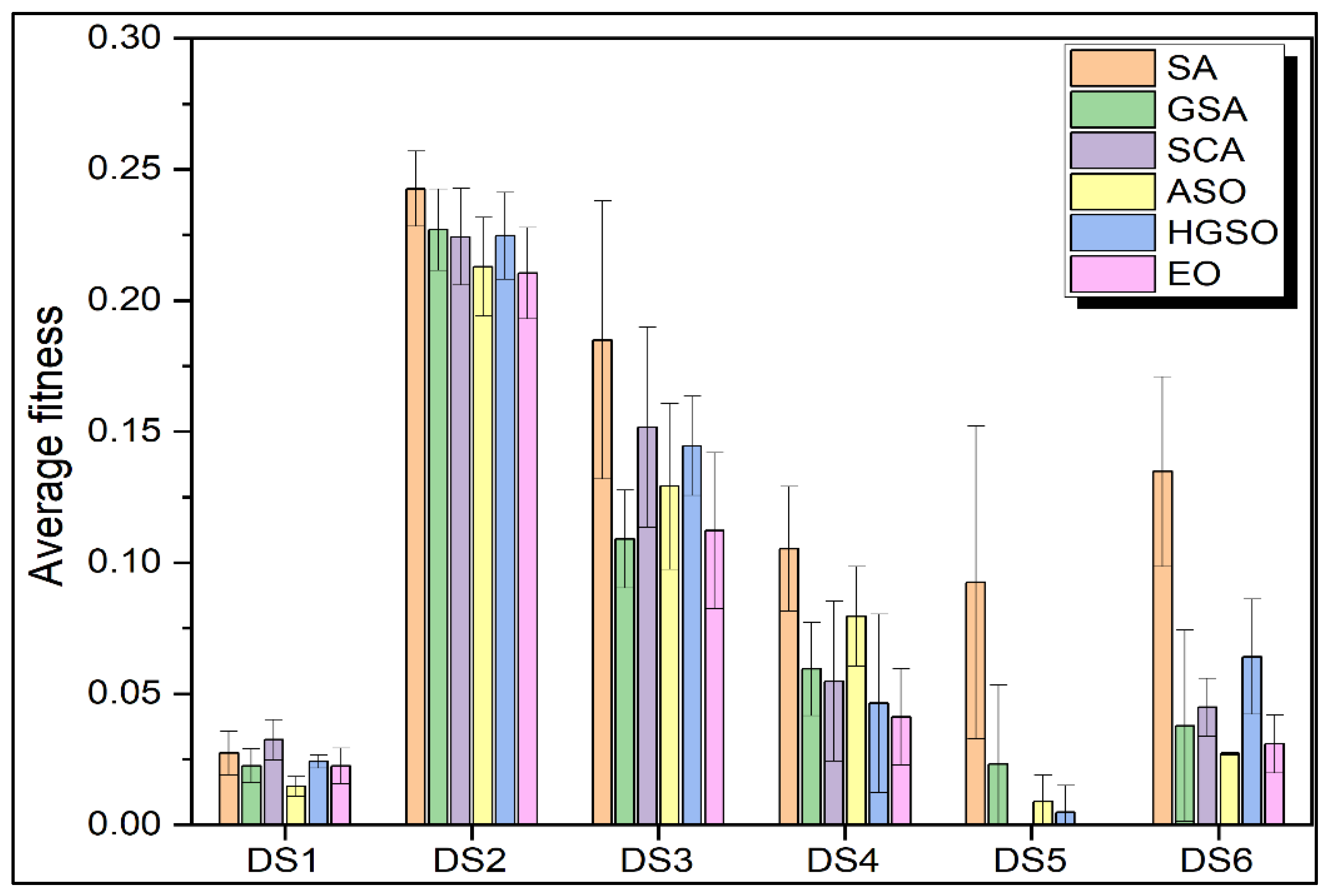
To have a clear picture and better understanding, the average fitness and standard deviation of each algorithm on all datasets are compared in Figure 2. The average depicts a slightly different picture. The average fitness of EO is no longer at rank 1 on DS1, DS3, and DS6; however, EO retained its rank in the case of DS2 and DS5. Furthermore, EO secured the first rank for the DS4, on which HGSO was better in the case of best fitness. On the contrary, HGSO could not maintain its performance. However, ASO maintained its performance on DS1 and outperformed the other algorithms on DS6. It is important to mention here SA was the worst performer in nearly all cases.

3.3.2. Comparison of Classification Accuracy

In this subsection, the classification accuracy and the average number of features selected by each algorithm are compared. The accuracy is the percentage of correctly classified test samples, and the average features selected (AFS) is the average number of features to which an algorithm reduces the dimensions of a dataset. AFS is computed by taking the average of the number of features selected by an algorithm in all 20 runs. The best accuracies obtained by each algorithm on all datasets are presented in Table 4. It is evident from the results that EO outperformed all other algorithms on all datasets. However, ASO performed equally well in three cases: DS1, DS5, and DS6. Simulated Annealing, on the other hand, was the worst performer on all datasets. It is important to note that the easiest dataset to classify was DS5, because all algorithms attained 100% on this dataset; however, SA was the only one that had an accuracy of less than 100% on this dataset. In this analysis, DS2 remained the toughest benchmark, on which the best performer could not obtain more than 82% accuracy.
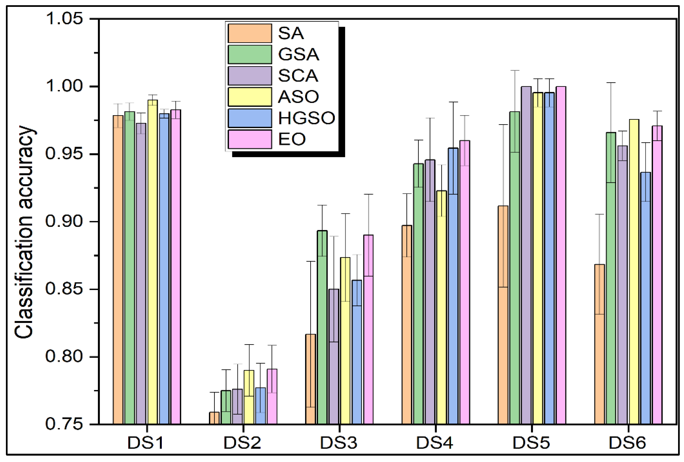
In addition to comparing best accuracies, the average accuracy of all runs along with standard deviations are compared in Figure 3. When comparing best accuracies, EO outperformed on all datasets, but due to inconsistent performance in different runs and a slightly higher standard deviation, EO was no longer the best performer on DS1, DS3, and DS6. However, its performance was comparable. On the other hand, ASO managed to outperform EO on DS1 and DS6, and both were equally good at DS2. Moreover, the performance of GSA was noticeably the best on DS3, whereas SA was still the worst performer on all datasets.
Finally, the average number of features selected by each algorithm (AFS) along with their standard deviations are presented in Table 5. As shown by the results, HGSO and SCA provided a minimum average number of features on two datasets each, whereas GSA and EO gave minimum AFS on one dataset each. However, if we also relate these results with the best accuracies, then the gain in terms of AFS of a few algorithms does not compensate for their low accuracies. For example, HGSO gave the minimum AFS on DS3, but its accuracy as compared to EO on DS3 was significantly low. Similarly, HGSO also gave the minimum AFS on DS6, but its accuracy was 2.5% lower than SCA, whereas the difference in AFS of both algorithms was just 0.2.
Amazingly, ASO, which gave some good results in terms of best accuracy, was unable to minimize dimensions as superbly as the other algorithms did. ASO frequently provided double the AFS as the best AFS provided by any other algorithm, as seen in DS2, DS4, DS5, and DS6.

3.3.3. Convergence Analysis

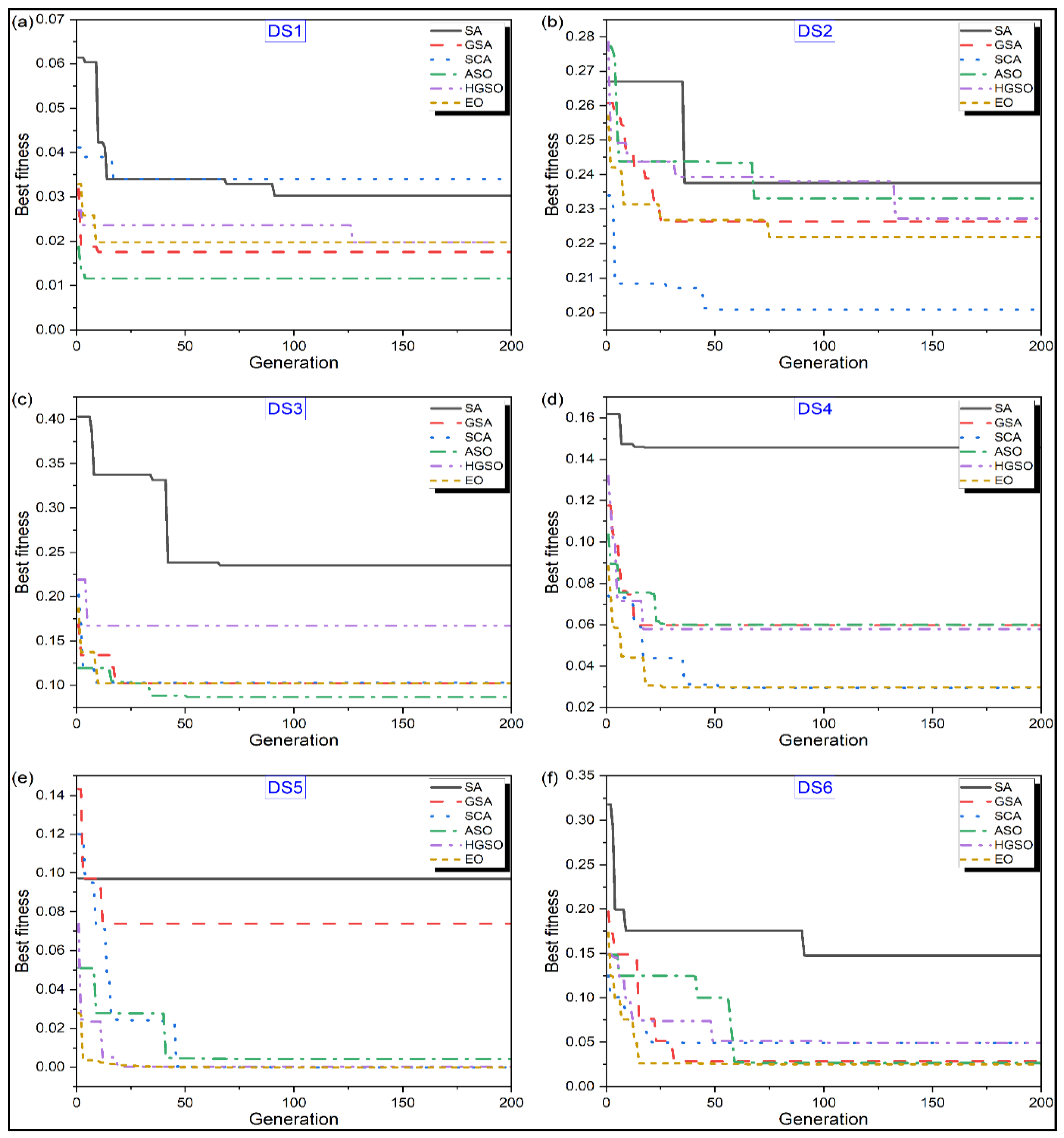
Convergence is the arrival of a stable point at which the solution stops improving any further. However, if an algorithm converges in very early iterations at a poor suboptimal point, then it is called premature convergence. In this section, we compare these algorithms based on how well they can converge, how well they can avoid premature convergence, and how quickly they can converge. The convergence curves of all these algorithms against each dataset are plotted in Figure 4. First of all, if we discuss the convergence capability, then all algorithms converged in less than the first half of the iterations for all datasets. If we talk about premature convergence, then SA converged prematurely in most cases; however, SCA on DS1, HGSO on DS3, and GSA on DS5 also converged prematurely. Finally, if we analyze their convergence speed, then EO demonstrated very good convergence speed on DS4, DS5, and DS6. In addition to that, ASO also demonstrated good speed on DS1 and DS3, and SCA was better than all the other algorithms on DS2. If we rank these algorithms based on the convergence capabilities, then EO secured the first rank, SCA was the second best, and SCA managed the third-best position.
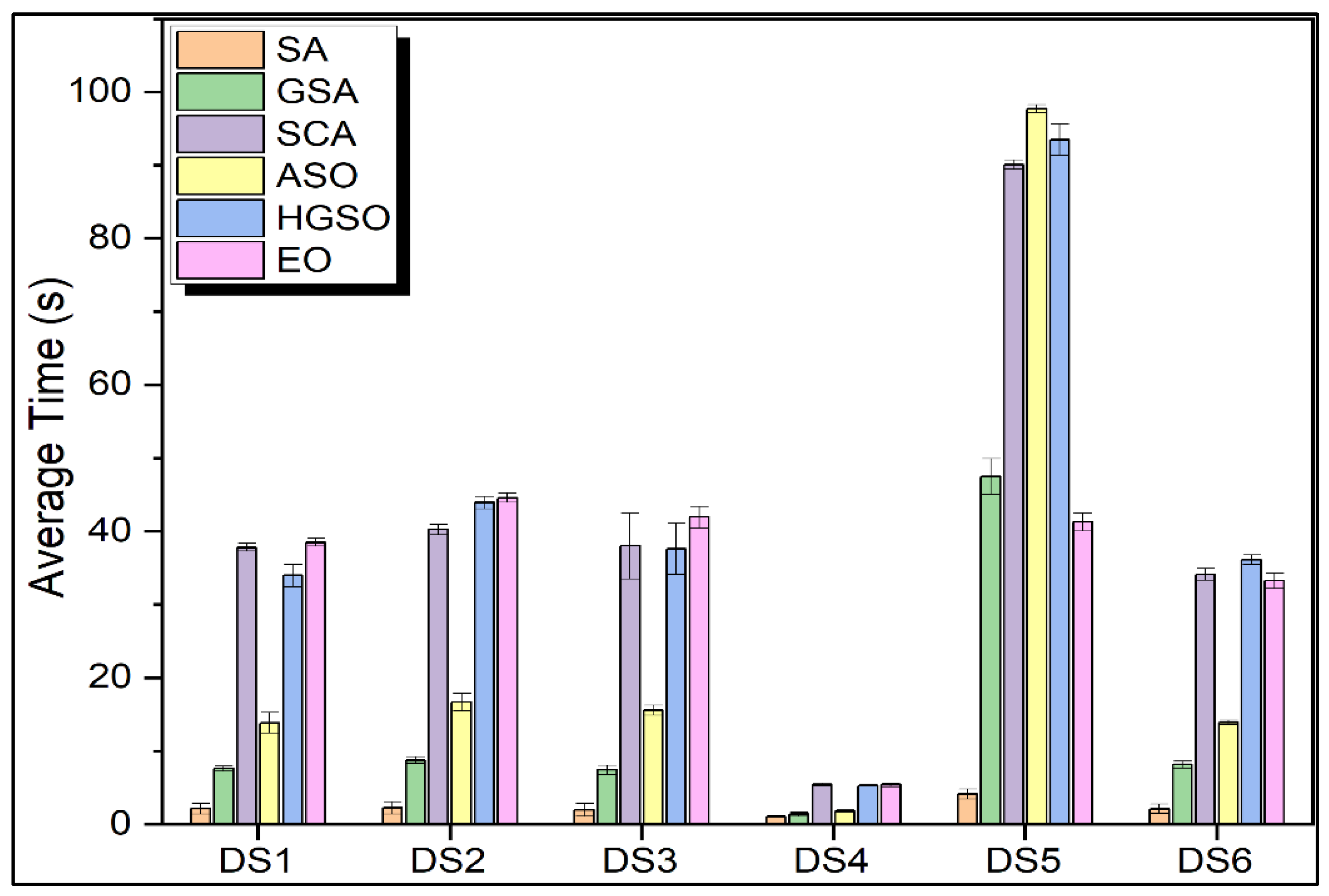
The convergence speed of all algorithms is also measured in the average number of seconds. The average computational time along with standard deviations are presented in Figure 5. The results showed that SA took the least amount of time to converge on all datasets, which is obviously due to its premature convergence. Another reason may be that it is a single-solution algorithm. Similarly, GSA was the second-fastest algorithm on five out of six datasets. However, if we talk about the computational time taken by the best performers such as EO and ASO, then ASO took much less time than EO on all datasets except DS5.

3.3.4. Overall Performance Analysis

To find the overall best algorithm, we computed the ranks of all algorithms from three perspectives: average fitness, average accuracy, and average features selected (AFS). Once the ranks were determined, the average rank of each algorithm was computed on all datasets. The overall ranks and average rank of all algorithms on each dataset are presented in Table 6. As the results illustrate, the best rank was attained by EO, which was 1.88. However, the second-best position was shared by SCA and HGSO. It is important to mention that SA was the worst performer on the list.

3.4. Comparison with Other Methods from the Literature

In this section, the top three physics-inspired metaheuristic algorithms are compared with the state of the art. For this comparison, results from other KNN-metaheuristic comminations reported by Elminaam et al. [37] were chosen. The metaheuristics chosen for comparison draw their metaphor inspiration from various sources. For example, the Grey Wolf Optimizer (GWO) and Whale Optimization Algorithm (WOA) may be classified as mammal inspired, whereas moth Flame Optimization (MFO) and the Butterfly Optimization Algorithm (BFO) are insect inspired. Similarly, Harris Hawk Optimization (HHO) and the Marine Predator Algorithm (MPA) are inspired by preying behavior seen in nature. Additionally, results based on popular ML algorithms such as Naive Bayes, Logistic Regression, Random Forest, Support Vector Machine (SVM), K-NN, Decision Tree, and Stochastic Gradient Descent (SGD) are also compared, along with their principal component analysis (PCA)-enhanced versions.
In terms of classification accuracy (Table 7), in two out of the three datasets compared, EO outperformed all the other methods. In fact, for the breast cancer dataset and ionosphere dataset, EO was on average 12.75% and 7.12% better, respectively, than the metaheuristics presented in [37]. In the sonar dataset, too, EO and SCA were within 2.5% of the best solution reported in [37]. Additionally, when compared with the ML algorithms, the EO solution for the breast cancer dataset was on average 17.89% better. An average superiority of 5.68% was seen for EO when compared with the PCA-ML methods reported in [38].
The average features selected for the breast cancer, ionosphere, and sonar datasets by the various metaheuristics are reported in Table 8. It can be observed that the feature reductions by the current physics-inspired metaheuristics are much higher. For the breast cancer, ionosphere, and sonar datasets, the average percent feature reduction achieved by the three physics-inspired algorithms was 85.11%, 88.24%, and 84.89%, respectively, and for the metaheuristic algorithms from [37], it was only 67.62%, 64.71%, and 67.14%, respectively.
Thus, from the comprehensive comparisons shown so far, it is clear that the current KNN hybridized physics-inspired metaheuristic algorithms (especially EO, SCA, and HGSO) are superior to those reported in the literature. Moreover, it is seen that even solutions by hybridized ML algorithms (for example, by dimensionality reduction techniques such as PCA) were inferior to current solutions. This is worth highlighting, since the current wrapper methods are much simpler in terms of computational complexity as compared to the PCA-hybridized ML methods.

4. Conclusions

In this paper, six well-cited physics-inspired metaphor algorithms were employed for feature selection. Feature selection is one of the major challenges being faced in the field of data mining and machine learning. The objective of this research was to identify the most promising physics-inspired algorithms for the problem of feature selection. To accomplish this, six small- to large-sized datasets were used. The performance of EO was found to be superior on most of the datasets, and the metrics that were used for the comparative analysis were taken from the literature and included accuracy, fitness, the average number of features selected, and convergence analysis. The current physics-inspired metaphor algorithms, especially EO, SCA, and HGSO comprehensively outperformed other metaheuristics, as well as the ML-based solutions seen in recent literature. Based on our findings, we highly recommend using EO for the feature selection problem.

Author Contributions

Conceptualization, R.Č. and K.K.; Data curation, J.P., M.P. and M.J.; Formal analysis, J.P., M.P. and M.J.; Investigation, J.P., M.P. and M.J.; Methodology, R.Č. and K.K.; Software, R.Č. and K.K.; Validation, J.P., M.P. and M.J.; Visualization, J.P., M.P. and M.J.; Writing—original draft, J.P., M.P. and M.J.; Writing—review and editing, R.Č. and K.K. All authors have read and agreed to the published version of the manuscript.

Funding

This research received no external funding.

Institutional Review Board Statement

Not applicable.

Informed Consent Statement

Not applicable.

Data Availability Statement

The data presented in this study are available through email upon request to the corresponding author.

Conflicts of Interest

The authors declare no conflict of interest.

References

  1. Köppen, M. The curse of dimensionality. In Proceedings of the 5th Online World Conference on Soft Computing in Industrial Applications (WSC5), Online, 4–18 September 2000; Volume 1, pp. 4–8. [Google Scholar]
  2. Ikotun, A.M.; Almutari, M.S.; Ezugwu, A.E. K-Means-Based Nature-Inspired Metaheuristic Algorithms for Automatic Data Clustering Problems: Recent Advances and Future Directions. Appl. Sci. 2021, 11, 11246. [Google Scholar] [CrossRef]
  3. Khalid, S.; Khalil, T.; Nasreen, S. A survey of feature selection and feature extraction techniques in machine learning. In Proceedings of the Science and Information Conference (SAI), London, UK, 27–29 August 2014; pp. 372–378. [Google Scholar]
  4. Porkodi, R. Comparison of filter based feature selection algorithms: An overview. Int. J. Innov. Res. Technol. Sci. 2014, 2, 108–113. [Google Scholar]
  5. Jović, A.; Brkić, K.; Bogunović, N. A review of feature selection methods with applications. In Proceedings of the 2015 38th International Convention on Information and Communication Technology, Electronics and Microelectronics (MIPRO), Opatija, Croatia, 25–29 May 2015; pp. 1200–1205. [Google Scholar]
  6. Brezočnik, L.; Fister, I.; Podgorelec, V. Swarm Intelligence Algorithms for Feature Selection: A Review. Appl. Sci. 2018, 8, 1521. [Google Scholar] [CrossRef] [Green Version]
  7. Askari, Q.; Saeed, M.; Younas, I. Heap-based optimizer inspired by corporate rank hierarchy for global optimization. Expert Syst. Appl. 2020, 161, 113702. [Google Scholar] [CrossRef]
  8. Rahman, A.; Sokkalingam, R.; Othman, M.; Biswas, K.; Abdullah, L.; Kadir, E.A. Nature-Inspired Metaheuristic Techniques for Combinatorial Optimization Problems: Overview and Recent Advances. Mathematics 2021, 9, 2633. [Google Scholar] [CrossRef]
  9. Mirjalili, S.; Mirjalili, S.M.; Lewis, A. Grey wolf optimizer. Adv. Eng. Softw. 2014, 69, 46–61. [Google Scholar] [CrossRef] [Green Version]
  10. Mirjalili, S.; Lewis, A. The whale optimization algorithm. Adv. Eng. Softw. 2016, 95, 51–67. [Google Scholar] [CrossRef]
  11. Passino, K.M. Bacterial foraging optimization. Int. J. Swarm Intell. Res. (IJSIR) 2010, 1, 1–16. [Google Scholar] [CrossRef]
  12. Whitley, D. A genetic algorithm tutorial. Stat. Comput. 1994, 4, 65–85. [Google Scholar] [CrossRef]
  13. Storn, R. On the usage of differential evolution for function optimization. In Proceedings of the North American Fuzzy Information Processing, Berkeley, CA, USA, 19–22 June 1996; pp. 519–523. [Google Scholar]
  14. Simon, D. Biogeography-based optimization. IEEE Trans. Evol. Comput. 2008, 12, 702–713. [Google Scholar] [CrossRef] [Green Version]
  15. Askari, Q.; Younas, I.; Saeed, M. Political Optimizer: A novel socio-inspired meta-heuristic for global optimization. Knowl.-Based Syst. 2020, 195, 105709. [Google Scholar] [CrossRef]
  16. Fadakar, E.; Ebrahimi, M. A new metaheuristic football game inspired algorithm. In Proceedings of the 2016 1st Conference on Swarm Intelligence and Evolutionary Computation (CSIEC), Bam, Iran, 9–11 March 2016; pp. 6–11. [Google Scholar]
  17. Rashedi, E.; Nezamabadi-Pour, H.; Saryazdi, S. GSA: A Gravitational Search Algorithm. Inf. Sci. 2009, 179, 2232–2248. [Google Scholar] [CrossRef]
  18. Hatamlou, A. Black hole: A new heuristic optimization approach for data clustering. Inf. Sci. 2013, 222, 175–184. [Google Scholar] [CrossRef]
  19. Zerigat, D.H.; Benasla, L.; Belmadani, A.; Rahli, M. Galaxy-based search algorithm to solve combined economic and emission dispatch. UPB Sci. Bull. Ser. C Electr. Eng. 2014, 76, 209–220. [Google Scholar]
  20. Abualigah, L.M.; Khader, A.T.; Hanandeh, E.S. A new feature selection method to improve the document clustering using particle swarm optimization algorithm. J. Comput. Sci. 2018, 25, 456–466. [Google Scholar] [CrossRef]
  21. Zakeri, A.; Hokmabadi, A. Efficient feature selection method using real-valued grasshopper optimization algorithm. Expert Syst. Appl. 2019, 119, 61–72. [Google Scholar] [CrossRef]
  22. Mafarja, M.M.; Mirjalili, S. Hybrid Whale Optimization Algorithm with simulated annealing for feature selection. Neurocomputing 2017, 260, 302–312. [Google Scholar] [CrossRef]
  23. Vijayanand, R.; Devaraj, D. A Novel Feature Selection Method Using Whale Optimization Algorithm and Genetic Operators for Intrusion Detection System in Wireless Mesh Network. IEEE Access 2020, 8, 56847–56854. [Google Scholar] [CrossRef]
  24. Kelidari, M.; Hamidzadeh, J. Feature selection by using chaotic cuckoo optimization algorithm with levy flight, opposition-based learning and disruption operator. Soft Comput. 2021, 25, 2911–2933. [Google Scholar] [CrossRef]
  25. Zawbaa, H.M.; Emary, E.; Parv, B.; Sharawi, M. Feature selection approach based on moth-flame optimization algorithm. In Proceedings of the 2016 IEEE Congress on Evolutionary Computation (CEC), Vancouver, BC, Canada, 24–29 July 2016; pp. 4612–4617. [Google Scholar]
  26. Selvakumar, B.; Muneeswaran, K. Firefly algorithm based feature selection for network intrusion detection. Comput. Secur. 2019, 81, 148–155. [Google Scholar]
  27. Abdel-Basset, M.; Ding, W.; El-Shahat, D. A hybrid Harris Hawks optimization algorithm with simulated annealing for feature selection. Artif. Intell. Rev. 2021, 54, 593–637. [Google Scholar] [CrossRef]
  28. Wolpert, D.H.; Macready, W.G. No free lunch theorems for optimization. IEEE Trans. Evol. Comput. 1997, 1, 67–82. [Google Scholar] [CrossRef] [Green Version]
  29. Too, J.; Liang, G.; Chen, H. Memory-based Harris hawk optimization with learning agents: A feature selection approach. Eng. Comput. 2021, 38, 4457–4478. [Google Scholar] [CrossRef]
  30. Bertsimas, D.; Tsitsiklis, J. Simulated annealing. Stat. Sci. 1993, 8, 10–15. [Google Scholar] [CrossRef]
  31. Mirjalili, S. SCA: A Sine Cosine Algorithm for solving optimization problems. Knowl.-Based Syst. 2016, 96, 120–133. [Google Scholar] [CrossRef]
  32. Zhao, W.; Wang, L.; Zhang, Z. Atom search optimization and its application to solve a hydrogeologic parameter estimation problem. Knowl.-Based Syst. 2019, 163, 283–304. [Google Scholar] [CrossRef]
  33. Hashim, F.A.; Houssein, E.H.; Mabrouk, M.S.; Al-Atabany, W.; Mirjalili, S. Henry gas solubility optimization: A novel physics-based algorithm. Future Gener. Comput. Syst. 2019, 101, 646–667. [Google Scholar] [CrossRef]
  34. Faramarzi, A.; Heidarinejad, M.; Stephens, B.; Mirjalili, S. Equilibrium optimizer: A novel optimization algorithm. Knowl.-Based Syst. 2020, 191, 105190. [Google Scholar] [CrossRef]
  35. Conrads, T.P.; Fusaro, V.A.; Ross, S.; Johann, D.; Rajapakse, V.; Hitt, B.A.; Steinberg, S.M.; Kohn, E.C.; Fishman, D.A.; Whitely, G.; et al. High-resolution serum proteomic features for ovarian cancer detection. Endocr.-Relat. Cancer 2004, 11, 163–178. [Google Scholar] [CrossRef] [PubMed] [Green Version]
  36. Street, W.N.; Wolberg, W.H.; Mangasarian, O.L. Nuclear feature extraction for breast tumor diagnosis. In Proceedings of the IS&T/SPIE 1993 International Symposium on Electronic Imaging: Science and Technology, San Jose, CA, USA, 31 January–5 February 1993; Volume 1905, pp. 861–870. [Google Scholar]
  37. Elminaam, D.S.A.; Nabil, A.; Ibraheem, S.A.; Houssein, E.H. An Efficient Marine Predators Algorithm for Feature Selection. IEEE Access 2021, 9, 60136–60153. [Google Scholar] [CrossRef]
  38. Ibrahim, S.; Nazir, S.; Velastin, S.A. Feature Selection Using Correlation Analysis and Principal Component Analysis for Accurate Breast Cancer Diagnosis. J. Imaging 2021, 7, 225. [Google Scholar] [CrossRef] [PubMed]
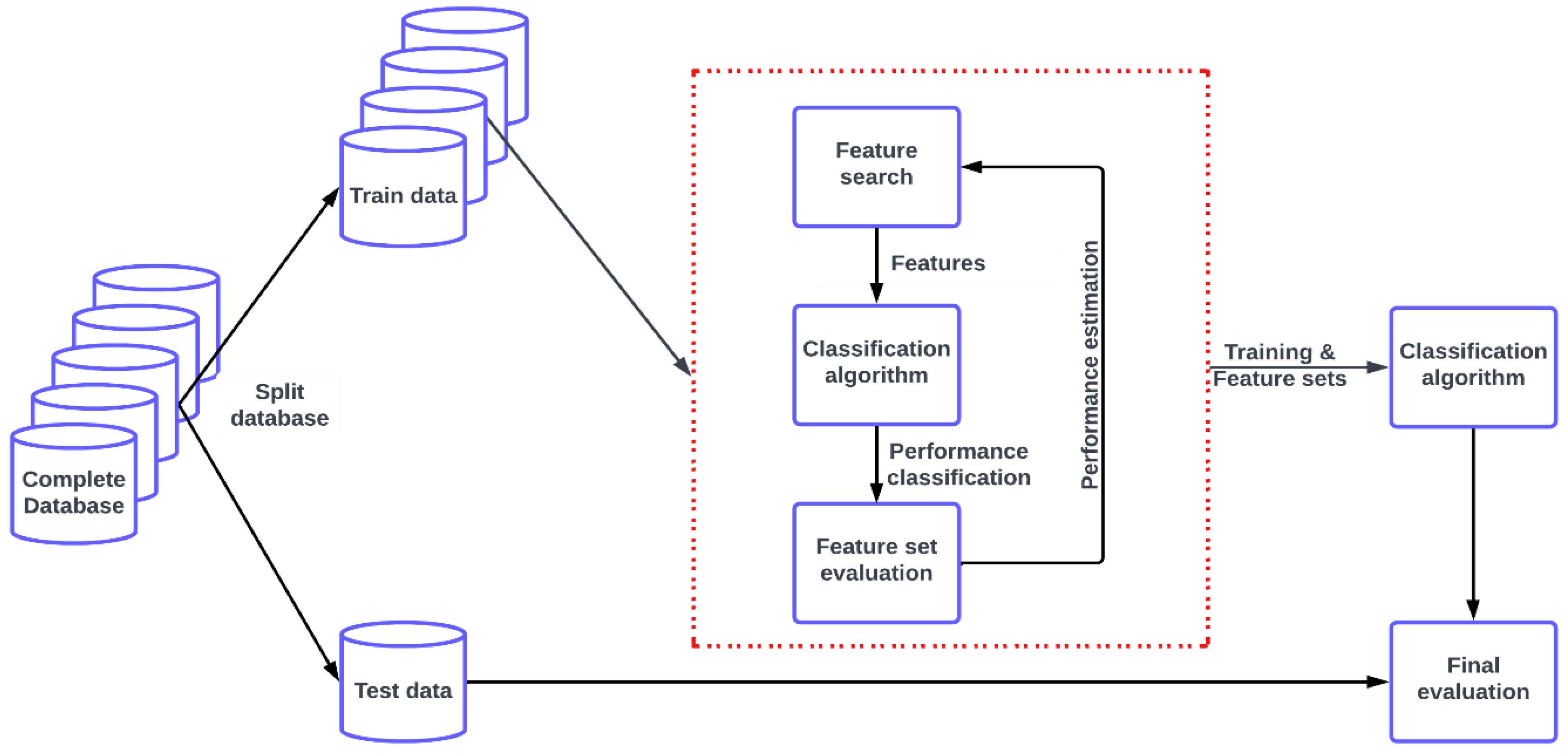
Figure 1. Wrapper feature selection framework.
Applsci 13 00906 g001
Figure 2. Average fitness and standard deviation of all algorithms on all selected datasets.
Applsci 13 00906 g002
Figure 3. Average classification accuracy and standard deviation of all algorithms on all selected datasets.
Applsci 13 00906 g003
Figure 4. Convergence curves of all algorithms on all selected datasets i.e., (a) Breast cancer (DS1) dataset, (b) German (DS2) dataset, (c) Heart (DS3) dataset, (d) Ionosphere (DS4) dataset, (e) Ovarian cancer (DS5) dataset, (f) Sonar (DS6) dataset.
Applsci 13 00906 g004
Figure 5. Average computational time and standard deviation of all algorithms on all selected datasets.
Applsci 13 00906 g005
Table 1. Datasets selected for this study.
DatasetSymbolNumber of InstancesNumber of FeaturesSource
Breast cancerDS156930https://archive.ics.uci.edu/ml/datasets/breast+cancer+wisconsin+(diagnostic), accessed on 12 September 2022
GermanDS2100024https://archive.ics.uci.edu/ml/datasets/statlog+(german+credit+data), accessed on 12 September 2022
HeartDS330313https://archive.ics.uci.edu/ml/datasets/heart+Disease, accessed on 12 September 2022
IonosphereDS435134https://archive.ics.uci.edu/ml/datasets/ionosphere, accessed on 12 September 2022
Ovarian cancerDS52164000Conrads et al. [35]
SonarDS620860https://archive.ics.uci.edu/ml/datasets/Connectionist+Bench+(Sonar,+Mines+vs.+Rocks), accessed on 12 September 2022
Table 2. Parameter settings of all algorithms.
AlgorithmParameterValue
Common for all algorithms k 5
Maximum iterations ( t m a x ) 200
Number of search agents ( N )30
Number of independent runs20
Ratio of validation data0.2
Simulated AnnealingCooling rate ( c )0.93
Initial temperature ( T 0 )100
Gravitational Search AlgorithmInitial gravitational constant ( G 0 ) 100
Constant, ( α ) 20
Sine Cosine AlgorithmConstant, ( α ) 2
Atom Search OptimizationDepth weight, ( α ) 50
Multiplier weight, ( β ) 0.2
Henry Gas Solubility OptimizationNumber of gas types2
K 1
Influence of other gas, ( α ) 1
β 1
l 1 0.05
l 2 100
l 3 0.01
Equilibrium Optimizer a 1 2
a 2 1
Generation probability0.5
V 1
Table 3. Best fitness values of all algorithms.
DatasetSAGSASCAASOHGSOEO
DS10.018690.017580.01980.011570.01980.01157
DS20.226920.202580.200920.192680.198880.18153
DS30.136620.086350.102850.087120.117810.06985
DS40.085740.044190.029460.059510.015320.01591
DS50.027980.004530.000010.004070.000010.00001
DS60.077770.003330.025150.026650.048630.02515
Table 4. Best classification accuracy of all algorithms.
Dataset SA GSA SCA ASO HGSO EO
DS10.985610.985610.985610.992810.985610.99511
DS20.7750.80.80.810.8050.82
DS30.866670.916670.90.916670.883330.93333
DS40.914290.957140.971430.942860.985710.98571
DS50.9767411111
DS60.9268310.975610.975610.951220.97561
Table 5. Mean selected feature subsets of all algorithms and their standard deviations.
Dataset SA GSA SCA ASO HGSO EO
DS1AFS
Std.
5.4
2.07364
3.6
0.54772
4.8
0.44721
4.2
0.83666
3.8
0.83666
4.8
0.83666
DS2AFS
Std.
9.6
1.81659
10.2
2.16795
6
1.41421
11.8
1.30384
9.4
3.91152
8.4
1.14018
DS3AFS
Std.
4.4
1.67332
4.4
0.54772
4
1.41421
4.8
1.09545
3.4
0.89443
4.2
0.83666
DS4AFS
Std.
11.6
4.92950
10
2.91548
3.4
0.89443
10.6
3.43511
3.6
1.14018
5
0.70711
DS5AFS
Std.
1986.6
37.35371
1891.8
73.07667
18
28.53945
1682.6
107.37225
77.2
60.95654
3.4
0.54772
DS6AFS
Std.
25.8
5.84808
23.8
4.14729
8
2.91548
17.8
3.11448
7.8
5.01996
11.4
4.15933
Table 6. Average rank of all averages (Fitness, accuracy, and AFS).
DatasetStats SA GSA SCA ASO HGSO EO
DS1Avg. fitness rank
Avg. accuracy rank
AFS rank
5
5
6
3
3
1
6
6
4
1
1
3
4
4
2
2
2
4
DS2Avg. fitness rank
Avg. accuracy rank
AFS rank
6
6
4
5
5
5
3
3
1
2
2
6
4
4
3
1
1
2
DS3Avg. fitness rank
Avg. accuracy rank
AFS rank
6
6
4
1
1
4
5
5
2
3
3
6
4
4
1
2
2
3
DS4Avg. fitness rank
Avg. accuracy rank
AFS rank
6
5
6
4
4
4
3
3
1
5
5
5
2
2
2
1
1
3
DS5Avg. fitness rank
Avg. accuracy rank
AFS rank
6
6
6
5
5
5
1
1
2
4
4
4
3
3
3
1
1
1
DS6Avg. fitness rank
Avg. accuracy rank
AFS rank
6
6
6
3
3
5
4
4
2
1
1
4
5
5
1
2
2
3
Avg. Rank5.613.663.113.333.111.88
Table 7. Comparison of classification accuracy with literature results.
MethodBreast Cancer% Improvement &Ionosphere% ImprovementSonar% Improvement
EO0.995Best Solution0.986Best Solution0.9762.46%
SCA0.9860.91%0.9711.54%0.9762.46%
HGSO0.9860.91%0.986Best Solution0.9515.15%
GWO [37]0.9702.58%0.9513.68%0.9703.09%
MFO [37]0.60564.46%0.77427.39%0.54782.82%
WOA [37]0.9732.26%0.9573.03%0.9762.46%
SSA [37]0.9821.32%0.9850.10%1.000Best Solution
BOA [37]0.90310.19%0.9019.43%0.88113.51%
HHO [37]0.9297.10%0.9296.14%0.83320.05%
MPA [37]0.9821.32%0.9850.10%0.9762.46%
Naive Bayes [38]0.84517.75%----
Logistic Regression [38] 0.87913.20%----
Random Forest [38]0.995Best Solution----
SVM [38]0.62060.48%----
K-NN [38]0.90010.56%----
Decision Tree [38]0.88013.07%----
SGD [38]0.90310.19%----
PCA-Naive Bayes [38]0.9752.05%----
PCA-Logistic Regression [38] 0.9752.05%----
PCA-Random Forest [38]0.9623.43%----
PCA-SVM [38]0.9425.63%----
PCA-K-NN [38]0.9218.03%----
PCA-Decision Tree [38]0.9059.94%----
PCA-SGD [38]0.9168.62%----
& % improvement achieved by the best solution with respect to the compared algorithms.
Table 8. Comparison of AFS with literature results.
MethodBreast Cancer% Feature
Reduction &
Ionosphere% Feature
Reduction
Sonar% Feature
Reduction
EO4.884%585%11.481%
SCA4.884%3.490%887%
HGSO3.887%3.689%7.887%
GWO [37]777%488%1182%
MFO [37]680%2332%3148%
WOA [37]873%779%2657%
SSA [37]1163%1459%1673%
BOA [37]1260%2041%2657%
HHO [37]1260%1071%2067%
MPA [37]1260%682%887%
& % Feature reduction is calculated as 100% minus the ratio of AFS by each algorithm and maximum features in the corresponding dataset. A higher value of % feature reduction is desired.
Disclaimer/Publisher’s Note: The statements, opinions and data contained in all publications are solely those of the individual author(s) and contributor(s) and not of MDPI and/or the editor(s). MDPI and/or the editor(s) disclaim responsibility for any injury to people or property resulting from any ideas, methods, instructions or products referred to in the content.