Abstract
The development of smart vehicles has increased the demand for high-definition road maps. However, traditional road maps for vehicle navigation systems are not sufficient to meet the requirements of intelligent vehicle systems (e.g., autonomous driving). The present work comes up with a method of generating high-definition map models based on the geographic information system (GIS). A systematic map construction framework including the road layer, intersection connection layer, and lane layer is proposed based on the GIS database. Specifically, the constrained Delaunay triangular network method is applied to extract road layer network models, which are then used as linear reference networks to construct lane-level road maps. To further examine the feasibility of the proposed framework, a field experiment is then conducted to build a high-definition road map. Furthermore, a lane-level map matching test is conducted in the constructed road map using the trajectory data collected from a probe vehicle. The results show that the proposed method provides an efficient way of extracting lane-level information from urban road networks and can be applied for lane-level map matching with good performance.
1. Introduction
In recent years, with the rapid development of smart driving technology, higher requirements are placed on the environmental perception and positioning accuracy of autonomous driving systems. Compared with road-level maps, high-definition maps not only provide rich lane-level data [1] and reduce the complexity of sensing but also help autonomous vehicles obtain accurate locations, with accuracy up to the decimeter or even centimeter level [2,3]. Moreover, high-definition maps can provide global path planning and navigation for smart vehicles based on stored information [4,5]. Therefore, high-definition maps are considered one of the core technologies of the perception layer and have developed into a key issue in the field of autonomous driving [6,7]. Although the significance of high-definition has been fully addressed during these years, existing research has not yet resulted in a method that can quickly and effectively build high-definition maps on the ground, so there is a need to continue to explore high-definition map construction methods and their applications in the field of intelligent transportation.
High-definition maps are pre-built digital models of the driving environment that provide an accurate description of road edges, lane lines, and other geometric shapes. According to the data sources, existing high-definition map construction technologies are generally divided into three categories: trajectory-based data, point-cloud-based data, and GIS-based data. The method based on trajectory data focuses on lane centerline extraction [8,9], which mines lane information by analyzing the shape features and directional features of a large number of global positioning system (GPS) trajectories and fits the lane lines utilizing spline curves and gyrus lines to achieve geometric modeling of lanes [10,11,12]. However, the accuracy of the lane geometry constructed using the methodology depends on the accuracy of the location of the detection vehicle, and the low-accuracy GPS trajectory is not sufficient to meet the requirements of high-definition maps. The point-cloud-based data approach is the most common and straightforward method to extract lane markings, based on the principle of 3D LiDAR combined with sensors such as positioning systems for acquisition, relying on road edges, and road lane markings to create environmental feature maps [13,14,15], or the point cloud data are transformed into georeferenced element images by Hough transform [16], multi-scale threshold segmentation [17,18], and multi-scale tensor voting (MSTV) to extract lane image schematics. The methodology can achieve higher accuracy; however, processing the entire LiDAR point can be time-consuming and its application is still hampered by the price of the sensors. Moreover, such a method requires intensive manual verification and regular maintenance [19], and building maps on a large scale is less efficient.
The GIS-based data approach uses road edge data obtained from GIS maps, and its construction is based on a linear reference system [20,21,22]. Compared with the above two methods, the construction of lane-level maps based on road boundary information obtained from GIS maps provides a lower cost and more efficient solution for large-scale high-definition map construction. Specifically, the road edge data provided by GIS maps can be used to extract the road centerline [23,24], which could be taken as a linear reference to generate lane lines [25]. Further steps can be taken to realize the construction of lane-level networks and the expression of topological relationships of the road network. Such a map construction method relies only on GIS maps without the additional acquisition of other high-precision sensing information [26], and thus has great advantages in terms of the map construction efficiency. In addition, the constructed map combined with the vehicle location information obtained by the global navigation satellite system (GNSS) and inertial measurement unit (IMU) could further realize lane-level map matching [19,27,28], so as to provide support for more refined lane-level traffic management and control, for instance, lane-level path navigation for smart vehicles. Despite the above-mentioned advantages, few studies have fully explored a systematic way of constructing high-definition road maps based on the GIS database.
Considering the urgent need of high-definition map construction for smart transportation applications and the importance of achieving high-efficiency in constructing high-definition maps for a large scale, the main objective of the present work is to explore effective methods of building high-definition maps based on the GIS and further prove its feasibility in supporting smart transportation applications. The major contributions of the present work can be summarized as follows:
- This study proposes a systematic framework and effective method for constructing high-definition maps using road edge data obtained from GIS maps. Through extracting the road centerline and the lane line and detailed expression of the topological relationship between nodes and lanes, a lane-level road network can be built. The proposed framework provides a low-cost and high-efficiency method for building lane-level road maps to support various smart city applications and refined traffic management.
- To further examine the feasibility of the constructed maps, a lane-level trajectory matching test is then conducted by taking the urban area of Pingshan District in Shenzhen, China as an example. The constructed lane-level maps based on the GIS could provide strong support for smart vehicle applications and lane-level traffic information management.
The rest of the paper is organized as follows: in Section 2, we first introduce the architecture of our proposed map model and then explain the relationship between road-level and lane-level maps. Section 3 introduces the algorithm of road centerline extraction and lane-level network construction. Next, we construct a lane-level road network model in Pingshan district in Shenzhen, China, and conduct lane trajectory matching tests based on the constructed real lane-level digital map, and evaluate the matching results in Section 4. Finally, we provide conclusions and directions for further research in Section 5.
2. System Framework for GIS-Based Map Construction
High-definition maps for smart vehicles should provide data support for driving environment data models for smart vehicle applications, and their lane-level road networks should contain detailed geometric and topological information of lane-level roads and intersections [29,30]. In order to design the lane-level road network model more efficiently, this paper integrates the real environment of smart vehicle driving and divides the map to be constructed into a road layer, lane layer, and intersection connection layer, as shown in Figure 1. The intersection connection layer clearly describes the topological relationship between the road layer and the lane layer.
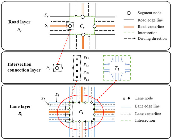
Figure 1.
Architecture of the map construction model.
2.1. Road Layer
The road layer describes the topological relationship among roadway segments and intersections. A road section line between two adjacent intersections is defined as a road segment, which describes a one-way or two-way connection between two adjacent intersections. Thus, the model of the road layer can be represented as Equation (1):
where is the road layer network, is all the intersection nodes in the network, is the centerline of all the road segments on the road, and is the road edge line. Road edge data describes the road width along with the road segment.
A road segment is composed of one or more lanes. For each segment in the segment set is identified by its ID and can be expressed as Equation (2):
where is the set of lane centerlines contained in the road segment, is defined as the road-level intersection node, and is the attributes of the road segment, including the road segment ID, the name of the road where the road segment is located, the road width, the length of each road segment, the number of lanes, and the direction of the road segment.
2.2. Lane Layer
The lane layer model is the set of lane segments and intersections and can be expressed as Equation (3):
where is the lane-level road network, denotes lane-level intersection nodes, denotes the centerline of all lanes on the road segment, and denotes lane edge lines.
In the lane centerline set , each lane centerline is identified by its ID, which can be expressed as Equation (4):
where indicates the node of a lane at the intersection, is the attributes of the lane centerline, including the lane centerline ID, the name of the road where the lane is on, the width, the length, the direction, and the left and right lane edge types.
The description of the lane edges in the lane layer is to better position the smart vehicle in the lane with width. In the lane edge collection , a single lane edge can be expressed as Equation (5):
where are defined the right lane and left lane adjacent to the lane boundary, respectively, and is the attributes of the lane edge, including the name of the road where the lane is located and the lane edge type.
2.3. Intersection Connection Layer
The intersection connection layer can be regarded as a connection layer between road-level information and lane-level information, which matches the lane-level information with the traditional road-level model. This layer includes road-level intersections and lane-level intersections.
A single intersection on a road can be expressed as Equation (6):
where is defined as the road segment node on the intersection, and denotes the topological relationship of different road nodes at the same intersection, which describes the connection between two roads, including two-way connections, one-way connections, and no connection.
A single intersection at the lane level can be expressed as Equation (7):
where is the set of lane nodes at the intersection, and denotes the topological relationship of different lane nodes at the same intersection. The lane-level topology relationship is represented according to the traffic rules at the intersection, including straight ahead, left turn, and right turn as well as unconnected lanes, as shown in Figure 2.
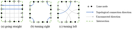
Figure 2.
Lane-level topology relationship.
The topological relationship between different lanes for the same road segment can be defined by using the inclusion relationship, as in Equation (8).
where is a single road segment node, the lane segment nodes contained in that road segment node .
3. Map Construction Method
While constructing a lane-level map based on the GIS map, a key step is to extract the road centerlines. In detail, we adopt the constrained Delaunay triangulation method to achieve the extraction of the road centerline [23]. Then, based on the extracted road centerlines, each lane line is further determined through the linear reference method considering the standard lane width. This section gives a description of these two steps.
3.1. Road Centerline Extraction
The core of extracting the road centerline is to detect the proximity relationship between boundaries. Delaunay triangulation as a method to construct the topological relationship of the data set that describes the interrelationship between data objects distinctly [31]. The road centerline extraction process based on Delaunay triangulation consists of three steps. First, the constrained Delaunay triangulation is constructed using densified road edge line points and road edge lines. Then, the road segments and intersection domains are extracted based on the constructed triangle network. Finally, the centerlines of the road segments and the intersection domains are then extracted.
3.1.1. Constructing Constrained Delaunay Triangulation
Compared with the traditional Delaunay triangulation, the construction of the constrained Delaunay triangulation required mandatory constraints on the polygon using the road edge nodes and line segments as constraints so that the road boundary becomes an edge in the triangle construction process [32]. For road areas, original points are often used to describe important morphological features of areas, such as inflection points and intersection points, and the number of these points is usually small. The construction of triangulation directly with constraints may generate some narrow and elongated triangles that do not correctly represent the proximity between polygons [33,34]. Hence, the densification of road points is required, as shown in Figure 3a.
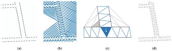
Figure 3.
Illustration of the steps to construct a constrained Delaunay triangle. (a) Points densification; (b) Constructing Delaunay triangulation; (c) Determination of road triangles; (d) Constructing CDT.
In general, the densification step is related to lane width, which can be set to 3–3.75 m. Considering the smoothness of the following road centerline connection, the road point densification step is set to 3 m in our experiment. The Delaunay triangulation is to be constructed using the point-by-point insertion method, and the schematic diagram of the construction is shown in Figure 3b. The basic idea of this method is to first find the minimum convex hull boundary containing the data region, then build the initial triangular network in it, and finally insert all the remaining points into the triangular network one by one [35] to ensure that it retains the Delaunay triangulation.
The triangulation constitutes a dissected structure in planar space, treating its basic unit as a single triangle. In order to identify the triangle within the road, the inclusion relationship between the center of gravity P of the triangle and the road area is taken as the judgment basis. In detail, if the gravity center of a triangle is located within the road, then the triangle is considered as a road triangle and needs to be retained. Otherwise, the triangle is not taken as a road triangle and needs to be removed. As shown in Figure 3c, when the center of gravity P1 is located within the road, then the blue triangle is a road triangle. In contrast, when the center of gravity P2 is not located within the road, then the gray triangle does not belong to the road triangle.
Then, all the road triangles are kept as the basis for road centerline extraction. The center of gravity of the triangle, which is calculated according to Equation (9), determines the inclusion relationship between itself and the road.
where are the horizontal coordinates of the three vertices of the triangle to be judged, are the vertical coordinates of the three vertices of the triangle to be judged, is the value of the horizontal coordinate of the center of gravity P of the triangle, and is the value of the vertical coordinate of the center of gravity P of the triangle.
The result of triangle extraction is shown in Figure 3d.
3.1.2. Road Division
In order to distinguish between road segment areas and intersection areas, it is necessary to classify road triangles. Road triangles can be classified into three types by the number of their neighboring triangles: if the triangle has only one neighboring triangle, it belongs to Type I, as shown in Figure 4a, which means this triangle is mainly located at the end of a road; if the triangle has two neighboring triangles, it belongs to Type II, as shown in Figure 4b, which means it is mainly located within a road segment; while if the triangle has three neighboring triangles, it belongs to Type III, as shown in Figure 4c, which means that it is located at the intersection. Based on such rules, the classification of the triangle types can initially be used to distinguish between road segment triangles and road intersection triangles.
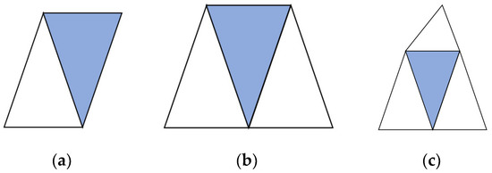
Figure 4.
Triangle-type division. (a) Type I; (b) Type II; (c) Type III.
To further delineate the intersection area, a circle with the road width as the radius is determined using the gravity center of the intersection triangle as the center of the circle. The intersection of the circle and the road edge is used as the road intersection boundary point (as shown in Figure 5a, the points ). These road intersection boundary points are connected in turn to determine the scope of the intersection.
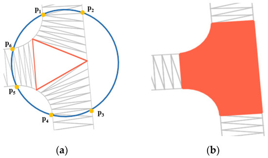
Figure 5.
Determination of the intersection area schematic. (a) Intersection boundary points; (b) Intersection scope.
3.1.3. Road Centerline Generation
The road centerline is composed of the road triangle centerlines. For type I triangles, the midpoint of one neighboring side and the midpoint of the longer side of the other two sides are calculated (e.g., P1 and P2 in Figure 6a). The two points are then connected to form the triangle centerline. For type II triangles, the midpoints of two neighboring sides are identified (e.g., P3 and P4 in Figure 6b). Then, P3 and P4 are connected to form the triangle centerline. For type III triangles, the gravity center of the triangle is first calculated (as P6 in Figure 5b), and the midpoint values of the three common sides are extracted (as P5, P7, and P8 in Figure 6b), and then, the center of gravity is connected to the other three points to form the centerline.
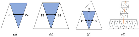
Figure 6.
Centerline construction in different types of triangles. (a) Type I; (b) Type II; (c) Type III; (d) Centerline construction.
The algorithm starts by traversing the adjacent triangles from any one of them and determines the next triangle to be visited based on the common edges. If the next triangle is a type II triangle, the midpoints of the two common edges are extracted and connected. If the next triangle is a type III triangle, extract the center of gravity and the midpoint of three sides of that triangle. When all the type I triangles have been searched once as the start or terminal points, and all the type III triangles have been searched three times as the start or terminal points, the network diagram construction is completed.
3.2. Lane-Level Network Construction
The lane-level road network is established based on the road-level network. The constructed road centerline is used as the linear reference network for generating the lane-level network. Based on the reference network, the geographic locations of lane-level data are generated and stored using a linear reference approach for the construction of lane-level road networks.
For data storage in GIS, the road data where each lane is located, the measured value of the lane start points and terminal points on the road, and the offset distance of the lane relative to the road will be recorded. The measured value indicates the distance from the start point of the reference line to a certain point along the direction of the reference line (as the distance from to in Figure 7), and the offset distance indicates the vertical distance from a certain point to the reference line, as shown in Figure 7 (the distance from to ). For a four-lane road with two directions, the right lane of the road centerline travels in the same direction as the road centerline, with a positive offset distance relative to the road centerline (as the o in Figure 7), while the left lane travels in the opposite direction, with a negative offset distance (as the -o in Figure 7). The specific calculation is expressed in Equation (10).
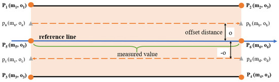
Figure 7.
Diagram of lane line extraction.
Here, the four points on the road edge (as in Figure 7) and the two points on the reference line (as in Figure 7) are called shape feature points. Each shape feature point has a corresponding reference value () in the linear reference system based on the road centerlines. According to the shape feature points of the road, the start point and the terminal point of each lane (shown as in Figure 7) can be identified.
where is the measured value of the lane start point and terminal point , is the offset distance of lane start points and terminal point , is the measured value of two adjacent shape points (e.g., in Figure 7) along the vertical direction of the reference line, and is the offset distance of two adjacent shape points (e.g., in Figure 7) along the vertical direction of the reference line. Usually, the offset value of the reference line is set to 0.
4. Experiment and Application: Lane-Level Trajectory Matching
4.1. Construction of a Lane-Level Road Network in Shenzhen
In order to evaluate the extraction results of the road network, we used part of the urban road network in Pingshan district in Shenzhen, China as an example. According to layer models of the high-definition map designed in Section 2 (shown in Figure 1), the road domain is divided and the centerline is extracted based on the constrained Delaunay triangular network method. The processing results are overlaid with the image map, as shown in Figure 8.
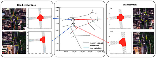
Figure 8.
Road division and road centerline extraction.
With the model framework and the methods introduced in previous sections, a lane-level network map is constructed, covering a domain of around 25 km2. As can be seen in Figure 9, the lane-level road network constructed in the present works matches well with the lanes shown in the image map.
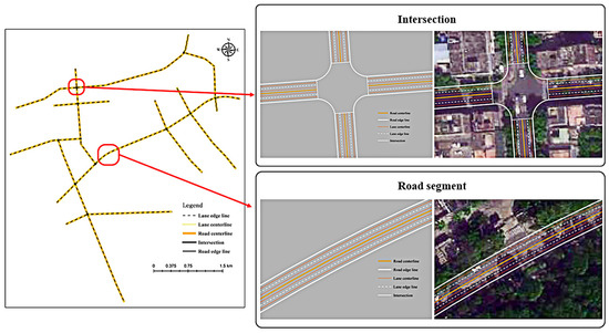
Figure 9.
A lane-level road network in Pingshan, Shenzhen.
4.2. Lane-Level Trajectory Matching
To further examine the feasibility of the constructed map in the applications of intelligent transportation services, a lane-level trajectory matching test is then conducted on the network. With the map sample constructed in the present work, a driving trajectory matching test was conducted. In the test, vehicle trajectory data and lateral driving behavior information are collected. Combined with the constructed high-definition map, the lane-level trajectory of the probe vehicle on the map is identified. Specifically, a u-blox F9 GNSS receiver and a front camera were adopted to receive IMU data and coordinate data and wheel speed information from the probe vehicle. Meanwhile, the lane-level trajectory of the probe vehicle was deduced using the detection results of lane-changing behavior via the smart vehicle driving process, which provides the platform for high-definition traffic monitoring, lane-level traffic control, and lane-level path planning of smart vehicles.
Lane-level trajectory matching consists of trajectory matching of road segments and road intersections. Specifically, trajectory matching in the road segment domain involves lane change trajectory smoothing with third-order Bezier curves and lane-keeping trajectory matching with orthogonal projections, and trajectory matching in the intersection domain includes turning trajectory matching with a lane-level topological map matching algorithm. The process of map matching and the specific experimental results are described in detail next.
4.2.1. Trajectory Matching in Road Segment Domains
Assuming that the starting lane of the collected trajectory is known, the trajectory points are searched according to the trajectory point time collection order. When a smart vehicle is driving along a road segment, if a lane change behavior is detected, towards which direction this lane change behavior occurs should be determined. While driving along a road segment, the vehicle’s trajectory is composed of lane change trajectory and lane keep trajectory. Figure 10 describes vehicle trajectory characteristics under the left lane change condition and the right lane change condition.
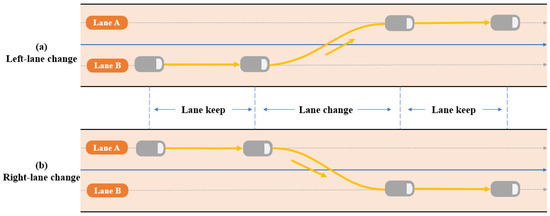
Figure 10.
The direction of a lane change.
In the present work, Bezier curves are used for the vehicle lane change trajectory model. The Bessel curve is used to smooth the trajectory connecting the start and end of the trajectory, which can represent a clear and simple relationship between the input control points and the generated curve, ensuring the smoothness, continuity, and controllability of the generated curve [36,37]. Considering that higher-order curves have higher computational costs, this paper adopts third-order Bezier curves to make the path curves more flexible and easier to realize the matching of the change of path trajectories.
Based on the lane change trajectory markers provided by the smart vehicle, two trajectory start points and two endpoints are selected as the control points of the trajectory change model in the trajectory change. The coordinates of each point on the third-order Bezier reference curve can be obtained using the following Equation (11):
where denotes the lane change path, denotes the time taken from to , and , , and denote the four required control points.
The control point can be expressed as Equation (12):
where denote the horizontal and vertical coordinates of control point .
As shown in Figure 11, the shape of the cubic Bessel curve is controlled by the four points , , , and . The curve starts from , moves towards and reaches from the direction of . The ends of the curve are determined by the start position and the end position of the vehicle lane change behavior. Control point and control point provide directional information and change the shape of the curve. The best matching result is achieved by setting the distance between and , and to set the channel change trajectory.
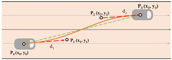
Figure 11.
Third-order Bezier curve channel change model.
For lane-keeping trajectory points on the road segment, the lanes that the trajectory points should be in are judged according to the start point of the vehicle and whether the lane-changing behavior occurs, and the trajectory points are matched to the centerline of the corresponding lane by orthogonal projection.
4.2.2. Trajectory Matching in the Intersection Domain
Intersection domain map matching is performed with a topological map matching algorithm (TMM). Our map data include lane-level topological relationships and construct a topological relationship graph with intersection nodes and directional edges to capture trajectories to the most appropriate edges using an if-then decision rule approach [38]. The algorithm defines a search area with a fixed radius around the estimated vehicle position. For the experiments, the search radius is set to 4 m. If the distance from a trajectory point to the centerline of a lane is larger than this threshold, this point will not be matched to this lane.
The basic idea of the algorithm is that the trajectory determines the lane node into the intersection, and based on this node, determines the possible path of the vehicle’s lane into the next lane. According to the lateral driving behavior of the intelligent vehicle at the intersection, the lane matched with the trajectory on next road section can be determined based on the topological relationship between each lane. As shown in Figure 12, if a vehicle arrives at an intersection through lane A, then the next lane it can access is predicted based on the lane nodes connected to lane A at that intersection (determined by the topological relationship between each lane at the intersection), which is shown as lane B and lane C. That is, if the vehicle goes straight at lane A, its trajectory at next road section will be matched to lane B. While if it turns left at lane A, then its trajectory at next road section will be matched to lane C. Similarly, if the vehicle reaches lane D, then next lane is probably Lane E or Lane F according to the topological relationship. At the intersection area, the next lane matched with the vehicle trajectory is analyzed based on the smart vehicle’s driving behavior of going straight or turning. The trajectory points are matched to the corresponding directional edges in the topology diagram through orthogonal projection.
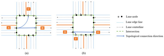
Figure 12.
Lane-level topological relationship at an intersection. (a) Topological relationship of lane A; (b) Topological relationship of lane D.
4.2.3. Trajectory Matching Test
In this experiment, the smart On-board Unit (OBU) device is mounted on the probe vehicle. The OBU is used as the data acquisition unit in the experiment, and its built-in ZED-F9K high-precision positioning module is capable of providing decimeter-level accuracy positioning data, as shown in Figure 13b. Moreover, the speed, acceleration, latitude and longitude, and wheel speed as well as other data obtained by using the IMU heading prediction module integrated into the device can provide crucial information for monitoring driving behavior such as lane changing behavior.
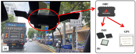
Figure 13.
Experimental platform. (a) Installation of the equipment; (b) Detailed components of OBU.
The device, shown in Figure 13a, was installed in the front windshield of the vehicle (a), while a camera recording was used during the test to probe the actual driving condition of the vehicle and provide a base for the subsequent trajectory verification. Based on the map constructed in the previous step, the test was run over the range of the constructed lane-level road network. The experimental test range is about 9 km long, covering part of the roads in Pingshan District, Shenzhen. The lane-level map covered during data collection is shown in Figure 14a, and a total of 14,928 trajectory points were acquired.
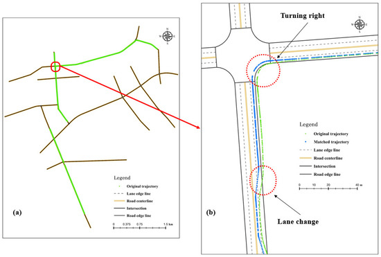
Figure 14.
Trajectory matching results. (a) The tested road sections; (b) Lane-level map matching results.
The trajectory coordinates are matched to the constructed lane-level network by the algorithm in Section 3. A sample map matching result for trajectory 2 is shown in Figure 14b.
In order to verify the effectiveness of the proposed method, the accuracy of the trajectory matching results is estimated by calculating the proportion of correctly matched trajectory points. Specifically, the trajectory matching accuracy rate R can be calculated through Equation (13).
where is the total number of correctly matched trajectory points for trajectory and represents all trajectory points covered in trajectory .
In our test, we have collected vehicle trajectory two times and the estimated trajectory matching accuracy are shown in Table 1.

Table 1.
Trajectory matching accuracy.
5. Conclusions
The present work proposes a high-definition map construction method based on the GIS. A map construction framework including the road layer, intersection layer, and lane layer is proposed. By making use of the road edge data provided by the GIS map, the constrained Delaunay triangulation method is adopted to extract the road centerline and to further recognize the intersection to build the road layer network. Then, the geographic locations of lane-level data are generated on the basis of a road-level network using a linear reference approach to build the lane-level network. Taking Pingshan district in Shenzhen, China as an example, a sample lane-level map covering a total area of 25 km2 is constructed. The detailed topology between each link and each lane is well explained in the constructed map. With this high-definition map, a lane-level trajectory matching test is further conducted to examine the feasibility of the proposed system. With the collected IMU data, GPS data, and probe vehicle lateral driving behavior, the trajectory of the vehicle is projected to the lane-level map using appropriate trajectory matching methods. The results showed that, with the help of the high-definition map, lane-level trajectory matching reaches an accuracy of over 96%. The outcomes of the present work provide a fast way of constructing lane-level road maps that could further support trajectory planning of smart vehicles and help in refining traffic management and control in smart cities. Considering the potential accuracy defects of the proposed system, further work will concentrate on validating the GIS-based map with vehicle trajectory data or other high-precision methods. Another potential direction could be the detailed expression of road networks with more complicated scenarios such as networks with roundabouts.
Author Contributions
Conceptualization, T.L., G.X. and X.Y.; methodology: T.L. and G.X.; data collection: T.L. and G.X.; analysis and interpretation of results: T.L., G.X. and X.Y.; draft manuscript preparation: T.L., G.X. and X.Y. All authors have read and agreed to the published version of the manuscript.
Funding
This research was partly supported by the Guangdong Basic and Applied Basic Research Foundation (No. 2020A1515111001), Guangdong University Engineering Technology Research (Development) Center (No. 2021GCZX002), Natural Science Foundation of Top Talent of SZTU (No. GDRC202130) and Cooperative R&D Project of SZTU (No. HKZLHT2022070322).
Institutional Review Board Statement
Not applicable.
Informed Consent Statement
Not applicable.
Data Availability Statement
The data is contained within the article.
Conflicts of Interest
The authors declare no conflict of interest.
References
- Liu, J.; Wu, H.; Guo, C.; Zhang, H.; Zuo, W.; Yang, C. Progress and Consideration of High Precision Road Navigation Map. Chin. J. Eng. Sci. 2018, 20, 99. [Google Scholar] [CrossRef]
- Gruyer, D.; Belaroussi, R.; Revilloud, M. Accurate lateral positioning from map data and road marking detection. Expert Syst. Appl. 2016, 43, 1–8. [Google Scholar] [CrossRef]
- Matthaei, R.; Bagschik, G.; Maurer, M. Map-Relative Localization in Lane-Level Maps for ADAS and Autonomous Driving; IEEE: Piscataway, NJ, USA, 2014; ISBN 9781479936373. [Google Scholar]
- Liu, C.; Jiang, K.; Yang, D.; Xiao, Z. Design of a Multi-layer Lane-Level Map for Vehicle Route Planning. MATEC Web Conf. 2017, 124, 3001. [Google Scholar] [CrossRef]
- Chaoran, L.; Kun, J.; Zhongyang, X.; Zhong, C.; Diange, Y. Lane-Level Route Planning Based on a Multi-Layer Map Model; IEEE: Piscataway, NJ, USA, 2017; ISBN 978-1-5386-1526-3. [Google Scholar]
- Zheng, L.; Song, H.; Li, B.; Zhang, H. Generation of Lane-Level Road Networks Based on a Trajectory-Similarity-Join Pruning Strategy. IJGI 2019, 8, 416. [Google Scholar] [CrossRef]
- Fernandez, F.; Sanchez, A.; Velez, J.F.; Moreno, B. Associated Reality: A cognitive Human–Machine Layer for autonomous driving. Robot. Auton. Syst. 2020, 133, 103624. [Google Scholar] [CrossRef]
- Zheng, L.; Li, B.; Yang, B.; Song, H.; Lu, Z. Lane-Level Road Network Generation Techniques for Lane-Level Maps of Autonomous Vehicles: A Survey. Sustainability 2019, 11, 4511. [Google Scholar] [CrossRef]
- Arman, M.A.; Tampère, C.M.J. Lane-level routable digital map reconstruction for motorway networks using low-precision GPS data. Transp. Res. Part C Emerg. Technol. 2021, 129, 103234. [Google Scholar] [CrossRef]
- Jo, K.; Sunwoo, M. Generation of a Precise Roadway Map for Autonomous Cars. IEEE Trans. Intell. Transp. Syst. 2014, 15, 925–937. [Google Scholar] [CrossRef]
- Gwon, G.-P.; Hur, W.-S.; Kim, S.-W.; Seo, S.-W. Generation of a Precise and Efficient Lane-Level Road Map for Intelligent Vehicle Systems. IEEE Trans. Veh. Technol. 2017, 66, 4517–4533. [Google Scholar] [CrossRef]
- Bender, P.; Ziegler, J.; Stiller, C. Lanelets: Efficient Map Representation for Autonomous Driving. In Proceedings of the IEEE Intelligent Vehicles Symposium Proceedings, Dearborn, MI, USA, 8–11 June 2014; IEEE: Piscataway, NJ, USA, 2014. ISBN 9781479936373. [Google Scholar]
- Ghallabi, F.; Nashashibi, F.; El-Haj-Shhade, G.; Mittet, M.-A. Dynamic Strategies Optimizing Benefits of Fully Autonomous Shared Vehicle Fleets LIDAR-Based Lane Marking Detection For Vehicle Positioning in an HD Map; IEEE: Piscataway, NJ, USA, 2018; ISBN 9781728103235. [Google Scholar]
- Hata, A.Y.; Wolf, D.F. Feature Detection for Vehicle Localization in Urban Environments Using a Multilayer LIDAR. IEEE Trans. Intell. Transp. Syst. 2016, 17, 420–429. [Google Scholar] [CrossRef]
- Jiménez, F.; Clavijo, M.; Castellanos, F.; Álvarez, C. Accurate and Detailed Transversal Road Section Characteristics Extraction Using Laser Scanner. Appl. Sci. 2018, 8, 724. [Google Scholar] [CrossRef]
- Yang, B.; Fang, L.; Li, Q.; Li, J. Automated Extraction of Road Markings from Mobile Lidar Point Clouds. Photogramm. Eng. Remote Sens. 2012, 78, 331–338. [Google Scholar] [CrossRef]
- Yan, L.; Liu, H.; Tan, J.; Li, Z.; Xie, H.; Chen, C. Scan Line Based Road Marking Extraction from Mobile LiDAR Point Clouds. Sensors 2016, 16, 903. [Google Scholar] [CrossRef] [PubMed]
- Guan, H.; Li, J.; Yu, Y.; Wang, C.; Chapman, M.; Yang, B. Using mobile laser scanning data for automated extraction of road markings. ISPRS J. Photogramm. Remote Sens. 2014, 87, 93–107. [Google Scholar] [CrossRef]
- He, M.; Rajkumar, R.R. LaneMatch: A Practical Real-Time Localization Method Via Lane-Matching. IEEE Robot. Autom. Lett. 2022, 7, 4408–4415. [Google Scholar] [CrossRef]
- Li Xiang, L.H.N. A trajectory-oriented carriageway-based road network data model, part 1: Background. Geo-Spat. Inf. Sci. 2006, 9, 65–70. [Google Scholar] [CrossRef]
- Li Xiang, L.H.N. A trajectory-oriented carriageway-based road network data model, part 3: Implementation. Geo-Spat. Inf. Sci. 2006, 9, 201–205. [Google Scholar] [CrossRef]
- Li Xiang, L.H.N. A trajectory-oriented carriageway-based road network data model, Part 2: Methodology. Geo-Spat. Inf. Sci. 2006, 9, 112–117. [Google Scholar] [CrossRef]
- Li, C.; Yin, Y.; Wu, P.; Wu, W. Skeleton Line Extraction Method in Areas with Dense Junctions Considering Stroke Features. IJGI 2019, 8, 303. [Google Scholar] [CrossRef]
- Lewandowicz, E.; Flisek, P. A Method for Generating the Centerline of an Elongated Polygon on the Example of a Watercourse. IJGI 2020, 9, 304. [Google Scholar] [CrossRef]
- Curtin, K.M.; Nicoara, G.; Arifin, R.R. A Comprehensive Process for Linear Referencing. URISA J. 2007, 19, 23–32. [Google Scholar]
- Sajeed, M.A.; Kelouwani, S.; Amamou, A.; Alam, M.Z.; Agbossou, K. Vehicle Lane Departure Estimation on Urban Roads Using GIS Information, Proceedings of the 2021 IEEE Vehicle Power and Propulsion Conference (VPPC), Gijon, Spain, 25–28 October 2021; IEEE: Piscataway, NJ, USA, 2021; pp. 1–7. ISBN 978-1-6654-0528-7. [Google Scholar]
- Shin, D.; Park, K.-m.; Park, M. High Definition Map-Based Localization Using ADAS Environment Sensors for Application to Automated Driving Vehicles. Appl. Sci. 2020, 10, 4924. [Google Scholar] [CrossRef]
- Kang, J.M.; Yoon, T.S.; Kim, E.; Park, J.B. Lane-Level Map-Matching Method for Vehicle Localization Using GPS and Camera on a High-Definition Map. Sensors 2020, 20, 2166. [Google Scholar] [CrossRef] [PubMed]
- Jiang, K.; Yang, D.; Liu, C.; Zhang, T.; Xiao, Z. A Flexible Multi-Layer Map Model Designed for Lane-Level Route Planning in Autonomous Vehicles. Engineering 2019, 5, 305–318. [Google Scholar] [CrossRef]
- Zhang, T.; Arrigoni, S.; Garozzo, M.; Yang, D.-g.; Cheli, F. A lane-level road network model with global continuity. Transp. Res. Part C Emerg. Technol. 2016, 71, 32–50. [Google Scholar] [CrossRef]
- Zhang, C.; Li, Y.; Xiang, L.; Jiao, F.; Wu, C.; Li, S. Generating Road Networks for Old Downtown Areas Based on Crowd-Sourced Vehicle Trajectories. Sensors 2021, 21, 235. [Google Scholar] [CrossRef]
- Paul Chew, L. Constrained Delaunay Triangulations. Algorithmica 1989, 4, 97–108. [Google Scholar] [CrossRef]
- Li, C.; Yin, Y.; Wu, P.; Liu, X.; Guo, P. Improved Jitter Elimination and Topology Correction Method for the Split Line of Narrow and Long Patches. IJGI 2018, 7, 402. [Google Scholar] [CrossRef]
- Zuo, Z.; Yang, L.; An, X.; Zhen, W.; Qian, H.; Dai, S. A Hierarchical Matching Method for Vectorial Road Networks Using Delaunay Triangulation. IJGI 2020, 9, 509. [Google Scholar] [CrossRef]
- Tsai, V.J.D. Delaunay triangulations in TIN creation: An overview and a linear-time algorithm. Int. J. Geogr. Inf. Syst. 1993, 7, 501–524. [Google Scholar] [CrossRef]
- Chen, L.; Qin, D.; Xu, X.; Cai, Y.; Xie, J. A path and velocity planning method for lane changing collision avoidance of intelligent vehicle based on cubic 3-D Bezier curve. Adv. Eng. Softw. 2019, 132, 65–73. [Google Scholar] [CrossRef]
- Zhang, F.; Xia, R.; Chen, X. An optimal trajectory planning algorithm for autonomous trucks: Architecture, algorithm, and experiment. Int. J. Adv. Robot. Syst. 2020, 17, 172988142090960. [Google Scholar] [CrossRef]
- Asghar, R.; Garzon, M.; Lussereau, J.; Laugier, C. Vehicle Localization Based on Visual Lane Marking and Topological Map Matching; IEEE: Piscataway, NJ, USA, 2020; ISBN 9781728173955. [Google Scholar]


Disclaimer/Publisher’s Note: The statements, opinions and data contained in all publications are solely those of the individual author(s) and contributor(s) and not of MDPI and/or the editor(s). MDPI and/or the editor(s) disclaim responsibility for any injury to people or property resulting from any ideas, methods, instructions or products referred to in the content. |
© 2023 by the authors. Licensee MDPI, Basel, Switzerland. This article is an open access article distributed under the terms and conditions of the Creative Commons Attribution (CC BY) license (https://creativecommons.org/licenses/by/4.0/).