Article

Bet-GAT: An Efficient Centrality-Based Graph Attention Model for Semi-Supervised Node Classification

1
Department of Computer Science and Engineering, Malaviya National Institute of Technology Jaipur, Jaipur 302017, Rajasthan, India
2
Department of Information Technology, Manipal University Jaipur, Jaipur 303007, Rajasthan, India
3
Department of Electronics Engineering, Veer Bahadur Singh Purvanchal University, Shahganj Road, Jaunpur 222003, Uttar Pradesh, India
4
Department of Computer Science, Electrical Engineering and Mathematical Sciences, Western Norway University of Applied Sciences, 5063 Bergen, Norway
*
Author to whom correspondence should be addressed.
Appl. Sci. 2023, 13(2), 847; https://doi.org/10.3390/app13020847
Submission received: 1 December 2022 / Revised: 28 December 2022 / Accepted: 30 December 2022 / Published: 7 January 2023
(This article belongs to the Special Issue Integrated Artificial Intelligence in Data Science)

Abstract

:
Graph Neural Networks (GNNs) have witnessed great advancement in the field of neural networks for processing graph datasets. Graph Convolutional Networks (GCNs) have outperformed current models/algorithms in accomplishing tasks such as semi-supervised node classification, link prediction, and graph classification. GCNs perform well even with a very small training dataset. The GCN framework has evolved to Graph Attention Model (GAT), GraphSAGE, and other hybrid frameworks. In this paper, we effectively usd the network centrality approach to select nodes from the training set (instead of a traditional random selection), which is fed into GCN (and GAT) to perform semi-supervised node classification tasks. This allows us to take advantage of the best positional nodes in the network. Based on empirical analysis, we choose the betweenness centrality measure for selecting the training nodes. We also mathematically justify why our proposed technique offers better training. This novel training technique is used to analyze the performance of GCN and GAT models on five benchmark networks—Cora, Citeseer, PubMed, Wiki-CS, and Amazon Computers. In GAT implementations, we obtain improved classification accuracy compared to the other state-of-the-art GCN-based methods. Moreover, to the best of our knowledge, the results obtained for Citeseer, Wiki- CS, and Amazon Computer datasets are the best compared to all the existing node classification methods.

1. Introduction

The role of Graph Neural Networks (GNNs) has grown significantly in the last 3–4 years for network mining and analysis [1]. Given the ever-evolving data on the social web and the dynamic evolution of network structures, GNN-based frameworks and explorations have improved significantly in contrast to other machine learning algorithms. In fact, Graph Convolutional Networks (GCNs) play a key role in the analysis and information mining of any kind of network structures (biomedical, electrical circuits, etc.). Tasks, such as semi-supervised classification of nodes [2], link prediction [3], graph classification [4], etc., achieve more promising results and predictions based on GCNs and GAT frameworks. The importance of these methods becomes even more apparent when considering that even with 20 % or less training data, model accuracy is much higher (over 75 % ) [2]. The node classification task is basically to find the mapping of nodes ‘N’ of a graph ‘G’ to the set of labels ‘L’. Mathematically, it can be expressed as G : N L . GCNs have been shown to be the most suitable models to perform the task of semi-supervised node classification in different networks. GCN is a message-passing algorithm on graphs. It means that the information about the graphical network propagates through the neighborhood interactions in the graph. In a semi-supervised classification task, the labels for a few nodes in the network are known. Based on this mechanism of message passing, the labels for the remaining nodes are determined. The machine-learning-based models or algorithms are able to use only the information based on the entity features. In contrast, GCN uses the neighborhood interactions, i.e., the information about the features of the node’s neighbours (as well as neighbours’ neighbours) along with the node features where neighbours are identified using edges. The idea of neighbourhood information aggregation to characterize the underlying node’s behaviour is the key aspect of GCN-based models. Thanks to this information propagation, GCN outperforms conventional machine learning models even for a small training dataset.
Graph Convolutional Networks (GCN) are preferable for the applications where data are generated from the non-Euclidean space with complex relationships and interdependencies. Traditional machine learning and deep learning strategies over graphical data tend to fail. These algorithms work well with structured data, with each data unit being independent of each other. Real-world networks, such as social networks, biological networks, road traffic networks, etc., are represented in the form of a graph. The graphical representations have an irregular structure where a node can have any number of neighbors. For example, in a social network, one user (node) can have ‘x’ number of users as friends in the network, while another user can have ‘y’ number of friends. Hence, the symmetry is not fixed as in the case of an image, where each pixel is represented as a fixed dimension. In addition, each user is related to its friends in the network, while in image data, each pixel unit is independent. In addition, the data for graphs are invariant to the node order. Hence, deep learning frameworks such as CNN are not suitable for operating over graphical data. GCNs do find their application in various application domains. Recently, the GCN framework has been utilized in Google Maps route optimization tasks. The route identification performed by converting the road network of a city into a graph and treating other road activities as features has experimentally shown traffic delays significantly optimized [5]. Protein Folding, another classical problem has also effectively utilized the predictive power of GCNs to estimate the protein molecule interactions. The proposed method not only improves predictions but also lowers the complexity of the task [6]. Similarly, GCN has extensive utility in various other fields, such as computer vision [7], natural language processing [8], medical imaging [9], VLSI domain [10], etc. With respect to a graphical network, the tasks that can be accomplished are node classification, link prediction, graph classification, graph clustering, etc. In this article, we consider the task of node classification to predict the label of a node in the network based on the aggregation of the information from its neighbor. The work presented in this article is an enhancement to the traditional GCN-based node classification in which the training dataset is chosen based on graphical properties of the node: (i) clustering coefficient and (ii) betweenness centrality. The proposed method, named Bet-GAT, accomplishes the task of node classification using the Graph Attention Model, which improves the classification accuracy of the traditional Graph Attention Model. Further, the proposed method attains improved results with a training dataset of around 20 % only, which is appreciable as feature availability for all the entities in a real-world network are a big challenge; hence, models need to work with a limited training dataset.
There are a number of studies based on GCN models to perform effective classification of nodes on different benchmark datasets. In this paper, we propose a network-centrality-based approach to select training set nodes for GCN and GAT models. The idea of GCN revolves around edge-connectivity-based information propagation and property transfer from node to node. Effective information propagation occurs in the network when important nodes are selected based on their structural position. We exploited this idea to select the training set such that nodes with high network centrality are selected [11]. Our results analysis of different benchmark networks shows that the validation and test accuracy improved significantly for these networks. The simulative analysis was performed for different centrality measures (degree, closeness, eigenvector, etc.). However, the best results are obtained by selecting the training sample betweenness centrality. This idea helps in accurate weight learning and in building the attention model. The results are promising for both binary and multiclass node classification tasks. The comparative analysis of the results with the other current methods proves the superiority of the proposed method.
The rest of the paper is organized as follows: Section 1 gives a brief introduction about GCN, its applications, and the contributions of the paper. Section 2 discusses in detail the modeling dynamics of GCN and GAT models. We also present the state of the art in graph theoretic models for deep learning, focusing on methods based on convolutional operations. Section 3 discusses how network centrality is helpful in improving the performance of GCN-based classification tasks. The section also defines the problem formulation, experimental setup, and algorithmic procedure and proposed framework. Section 4 is the results and analysis section. This section highlights the behavioral aspects of the proposed model. We also present the performance evaluation of the proposed method by comparing our results with the other prominent current methods. Section 5 summarizes our main contributions.

2. Literature Survey

In this section, we present the basics of Graph Neural Networks (in particular GCN and its variant GAT) along with an extensive literature review on these methods.

2.1. Graph Convolutional Neural Networks (GCNs)

Graph Convolutional Networks are the type of neural networks that work directly with graphs. The idea of Graph Convolution is analogous to Convolutional Neural Networks (CNNs) for images. The main difference between CNNs and GCNs is that CNNs work with regular Euclidean (structured) data, while GCNs work with data in non-Euclidean space. This is due to the irregularities in the network structure caused by the different neighborhood connections and alignments. Therefore, the operational feature extraction method is different from the one used for CNNs. Therefore, we need a mathematical model formulation based on spectral graph theory to solve the problem.
The convolution operation defined for an image using CNNs introduces hidden convolution and pooling layers to identify spatially localized features via a set of receptive fields in kernel form. We slide the convolutional operator window across a two-dimensional image, and we compute some function over that sliding window. Then, we pass it through many layers. Convolution takes a little sub-patch of the image (a little rectangular part of the image), applies a function to it, and produces a new part (a new pixel). The center node of that center pixel aggregates information from its neighbors, as well as from itself, to produce a new value. However, the same strategy cannot be utilized for GCNs due to the arbitrary size of the graph and the complex topology, which means there is no spatial locality. The structural differences are depicted in Figure 1. In addition, the convolution operation must be invariant to node order. For GCNs, the challenging task is to identify an encoding function which can encode the nodes of a graph in a d-dimensional space preserving the proximity of nodes as in the original graph (local network neighborhoods). Based on this, the computational graph for each node is defined, and aggregation of information is performed for a particular node. Thus, we have convoluted information aggregated over each node of the network.
Here, we consider the problem of node classification by GCN. The general idea of GCN is to collect information about the neighborhood of a node for which the class is to be predicted. This includes both the local neighborhood information and the characteristics of the individual node, which serve as input to the model. Let us build the model based on this information. Let G be an undirected graph with V a set of nodes such that v i ϵ V and let E be the set of edges such that ( v i , v j ) ϵ E . Furthermore, let X be the feature vector corresponding to each node in N. From this, the aggregation function can be defined as follows:
Z = f   ( A , X ) = A × X
in which A is an adjacency matrix, such that A ϵ R N X N , X is the feature vector matrix, such that X ϵ R N X C , N is the number of nodes in the network, C is the dimensions of the feature vector, and λ is S c a l a r ( λ > 0 ) .
Equation (1) represents the sum of all neighborhood vectors except itself. For this purpose, consider a self-loop for each node:
A ^ = A + λ I N
Thus, the final aggregated function becomes:
Z = A ^ × X
To prevent the dominance of feature vectors, the function is normalized using the degree matrix. The degree matrix over the graph ‘G’ with adjacency matrix ‘A’ is defined as: D i , i = j A i j . Using this information, the aggregate convolution function is defined as [2]:
Z = f ( A , X ) = D 1 / 2 A ^ D 1 / 2 × X
The adjacency matrix is scaled over both rows and columns. This provides the weighted average scaled uniformly both for low and high degree nodes. For a 2-layer GCN, where the first layer is an input layer and the second is the output layer, as given in Equation (1), the forward model is defined as [2]:
Z = f ( A , X ) = s o f t m a x ( A ^ . R e L U ( A ^ × X × W ( 0 ) ) × W ( 1 ) )
Here, A ^ is defined as D 1 / 2 × A × D 1 / 2 . The ultimate task is to learn the weights for the model where C × H are the trainable weights for W ( 0 ) (weights at layer 0). Similarly, H × F trainable weights for W ( 1 ) (weights at layer 1). Here, C refers to the dimensions of the feature vectors, F refers to the dimensions of the resulting vectors and H is the number of hidden layers. The expression in Equation (5) can further be extended depending upon the hidden layers in the network. The depth of the network is based on the intuition of the k path length neighborhood contribution. However, in general, graph networks do not have much effect of the neighborhood interactions beyond 2–3 path lengths [12]. Thus, results of 2–3 layer GCN networks are considerable and impressive. Further, considering the neighbors beyond this range spoils the meaning of neighborhood aggregation, and the results will overfit.
The last layer of the GCN corresponds to the number of classes for which the prediction is to be made. The output vector of the last layer is then passed through a Softmax function to make the predictions. The cross entropy loss function is used for training:
L = y ϵ Y l f = 1 F Y l f l n Z l f
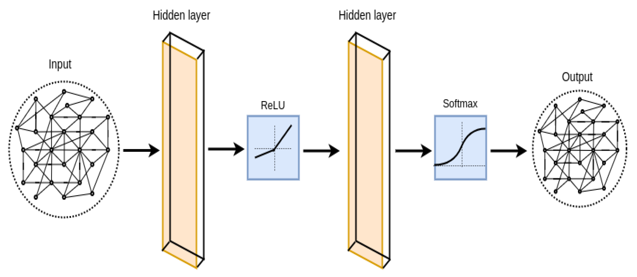
Here, Y I is the set of node indices with labels. The whole discussion so far summarizes the process (Figure 2) of semi-supervised node classification by the GCN model. The training process is tuned using hyperparameters such as learning rate, number of layers of the network, number of epochs, dropout, etc., to optimize the loss function as per Equation (6).
Graph Neural Networks have been the most widely studied area of research in recent years. These are specific types of neural networks based on the graph structure. The semi-supervised node classification using the GCN model was proposed by Kipf et al. [2]. This GCN model is capable of encoding node features and underlying graph structure. A new GCN approach, Graph Wavelet Neural Network (GWNN) [13], significantly outperforms spectral graph CNNs in the task of graph-based semi-supervised classification. Abu-El-Haija et al. [14] proposed a model using multiple powers of an adjacency matrix. Lu et al. [15] addressed the attention mechanism problem for multiple prediction tasks, such as node and graph classification. Several studies worked on the performance improvement of GNNs [16,17].
For performance improvement of semi-supervised classification, Lin et al. [18] proposed an SF-GCN structure fusion model that is based on graph convolutional networks. Another approach by Gao et al. [19] conveys the learning graph convolutional layer (LGCL), which takes out a fixed number of neighbor nodes for each feature and transforms graph data into grid-like structures. In contrast to these methods, Luo et al. [20] focused on a novel framework called Self-Ensembling GCN (SEGCN), where both labeled and unlabeled nodes were used to train GCN. For the same scenario, Franceschi et al. [21] incorporated the graph structure and parameters of graph convolutional networks. Zhou et al. [22] addressed the shortcomings of the GNN architecture through the automated Graph Neural Networks (AGNN) framework. Gao et al. [23] also developed a graph neural architecture search method. Jiang et al. [24] defined Graph Optimized Convolutional Network (GOCN) for graph data representation and learning, which is applicable to multiple graphs.
Wijesinghe et al. [25] used Distributed Feedback-Looped Networks (DFNets) for the spectral convolutional neural network. Recently, Dabhi et al. [26] proposed a model using NGL-NodeNet to solve node classification tasks for citation graphs. Huang et al. [27] trained GCNs for large graphs by implementing an adaptive layer-wise sampling method. More recently, Wang et al. [28] developed an end-to-end model that defines the incorporation of GCN and a Label Propagation Algorithm (LPA) for node classification. This model allows simultaneous learning of transformation matrices and edge weights. Therefore, it provides better performance compared to a traditional GCN.

2.2. GCN to GAT Transition

GCNs, the simplest formulation of Graph Neural Networks, define model training based on the concept of isotropic aggregation. Isotropic aggregation means that the contribution of each neighbor to the node under consideration is considered equal. On this basis, the simple neighborhood aggregation function is defined as follows [24]:
h v k = σ ( W k [ Σ u ϵ N ( v ) h u k 1 N ( v ) ] + B k . h v k 1 )
Equation (7) is a more formalized way of expressing a GCN model. Here, h v k represents the resulting node embedding after k layers of neighborhood aggregation, σ represents the nonlinear function (e.g., ReLU), h u k 1 represents the node embedding of the previous layer, Σ u ϵ N ( v ) h u k 1 N ( v ) is the average neighborhood aggregation over u nodes such that u ϵ N ( v ) , and B k is the bias.
The Graph Attention Model varies the concept of GCN by defining the importance of neighborhood connections. It defines the importance of the message from node u to node v such that ( u , v ) ϵ E . Let a define the attention coefficient for the edge e v u for the pair of nodes ( u , v ) ; e v u is defined as [24]:
e v u = a ( W k h u k 1 , W k h v k 1 )
Furthermore, normalizing the expression in Equation (8) using the Softmax function, the equation turns out to be:
α v u = e x p ( e v u ) k ϵ N ( v ) e x p ( e v k )
Finally, the node embedding at K t h layer is defined as:
h v k = σ ( u ϵ N ( v ) α v u W k h u k 1 )
Equation (10) defines the learning model according to GAT. The parameters of the attention mechanism a are trained using a neural network. These parameters are learned together with the weight matrices. To stabilize the learning process, a multi-head attention mechanism is used. Here, the attention operations for each layer are repeated R times independently. Finally, the output is aggregated or summed. This equation-based analysis of the process justifies why GAT has an advantage over GCNs. GAT considers aggregation of neighbors based on their importance with respect to the node. This further improves the accuracy of the results and the quality of the learning process imparted to the model.
In the world of neural network architectures running on graph structure data, Veličković et al. [29] introduced a new approach called GATs, i.e., Graph Attention Networks. The authors try to strengthen GCN approximation techniques and remove weaknesses by using mask self-attention layers. In this model, nodes can pick up information about neighboring nodes by superimposing the layers. Interestingly, no prior knowledge of graph structure is required to implement layering, and this process is computationally fast.
Yu et al. [30] present a supervised graph attention network (super- GAT). This model considers both implicit and explicit weights for the nodes. Therefore, the model provides better results than the traditional GAT. In another robust variant of GAT, Shanthamallu et al. [31] claim that the performance of semi-supervised learning is improved. In refining GAT, Wang et al. [32] focused on overfitting during training and improved the performance of their model.

3. Proposed Methodology

3.1. Background of Network Centrality Measures

The concept of network centrality was first discussed in [33]. In a network, identifying the most important nodes is a very important task in order to efficiently control the flow of information. In a graphical network, a few nodes are positioned in the network in such a way that they define communication paths for the nodes at the periphery of the network. Due to their optimal structural position in the network, their reachability to different parts of the network and their accessibility from other nodes are high. As can be seen in Figure 3, the central node has the highest centrality value due to its better accessibility to other nodes (in terms of path length).
However, the notion of importance for the nodes in the network depends on the choice of the task to be accomplished. In some cases, the node with the most connections in the network is important, while in other cases, the node through which most edge connections pass is more important. Based on these criteria, there are different types of network centrality measures.
When measuring degree centrality, nodes with more links in the network [34] are given higher importance. Alexander Bavelas [35] was the first to introduce closeness centrality. Degree centrality may not be a good criterion for defining the importance of a node in the network. Closeness centrality defines the importance of a node based on the notion of closeness to other nodes. However, this was later redefined as harmonic centrality [36] because the functional definition for closeness centrality is not valid for an unconnected network. The computation of Eigenvector centrality for a node is based on what kind of nodes the underlying node is connected to [37].
The betweenness centrality metric [38] is a path-based measure based on two conjectures: node betweenness and edge betweenness. The latter, however, depends on the node betweenness. Here, the importance metric of the node depends on how often it occurs on the shortest paths from one node to another. We then can obtain Equation (11) as:
c b e t ( x ) = y , z x , σ y z 0 σ y z ( x ) σ y z
Here, σ y z stands for the number of shortest paths from y to z and σ y z ( x ) for the number of these paths passing through x. The centrality measure has several implications for finding the important nodes in the network when the flow of information between two groups is mediated by a node or group of nodes. Brandes [39] proposed an efficient algorithm for computing betweenness centrality. The time complexity of Brandes’ algorithm is O ( n m + n 2 l o g n ) , and the space complexity is O ( n + m ) , where n and m are the number of nodes and edges in a graph, respectively.
These are some basic centrality measures to identify the important nodes of the network based on their structural positions. Current research further explores the applicability and usability of centrality measures depending on the network structures and applications. In this proposed work, we use this concept to identify a set of nodes for training the Graph Neural Network. To improve the training dataset, we choose nodes with high betweenness centrality values. In the next subsection, we justify this statement with a detailed analytical reasoning.

3.2. Justification of Betweenness Centrality Based Training

Let us consider a network in terms of a graph G ( V , E ) such that V is the set of vertices or nodes defined as v 1 , v 2 , , v n V , and E is the set of edges or links defined as e 1 , e 2 , , e k E such that n, k > 1 .
Let X be the feature matrix of order n × m defined for each node v i V . Thus, the feature matrix’s row will be given as: x 1 , x 2 , , x m x i ∈ X such that 1 < i < m . Generally, we have n > m (size of training data > size of feature vector for each node) in order to avoid the condition of overfitting during the training process. We consider total p different classes ( c 1 , c 2 , , c p ) for the underlying node classification problem; i.e., each node v i belongs to one of these p classes which is represented by its label l i associated with it; l i c 1 , c 2 , , c p where p < < n . Consider the optimal label set L, where each node has its correct classification label; i.e., the correct class value is known for all the nodes.
So far, we have defined all the basic terminologies of our proposed model. Our goal is to identify a mapping (predicted label set) that is close to the optimal set L. We need to show that the classification accuracy of the GAT model improves when nodes with high betweenness centrality are chosen as training nodes for the model. For this, we need to show two things:
(1)
A subset of training nodes selected based on betweenness centrality improves training efficiency.
(2)
The probability of selecting the same subset of nodes by a traditional GAT/GCN model (by default random selection of training nodes) is near zero.
Let us consider the first statement and infer its validity. A subset of training nodes selected based on betweenness centrality improves training efficiency.
For GCN and GAT as per Section 2.1 and Section 2.2, we already know that the model accuracy depends on the neighborhood aggregation. In other words, neighborhood aggregation contributes to more and more availability of features for training the data. We can say that training efficiency ∝ feature availability ∝ neighborhood aggregation.
Thus, the problem reduces to finding an efficient subset of nodes that can increase the availability of features. Let A″ be a subset of nodes defined over the set V such that nodes are selected in order of betweenness centrality score. Let A be another subset of nodes from the set V such that the nodes are randomly selected. Here c a r d i n a l i t y ( A ) = c a r d i n a l i t y ( A ) is maintained. Suppose the very first node (with the highest betweenness centrality) a A is selected, and the first node in b A is selected. Since the nodes in A are selected based on betweenness centrality, the following holds,
betweenness centrality score(a) > betweenness centrality score(b)
We assume that a b , i.e., that the same node a is not selected by the random selection process. The reason is that the probability of the node a being selected by the random process is 1 / n , which is close to zero for large values of n.
According to the definition of betweenness centrality from Section 3.1, a node with a high betweenness centrality value participates in a larger number of shortest paths between different pairs of nodes of the graph. This implies that:
Number of shortest paths with membership of node a > Number of shortest paths with membership of node b
It should be noted that node coverage up to q path length should be considered, where q > 0 , and generally has a small value. For GAT, the neighborhood contribution is not taken into account for a path length of two hops or more. Thus, we can say that node a necessarily has more neighbor nodes of path length p compared to node b. This is because a participates in more shortest paths compared to b, and from this it can be deduced that:
node coverage(A″) > node coverage (A′)
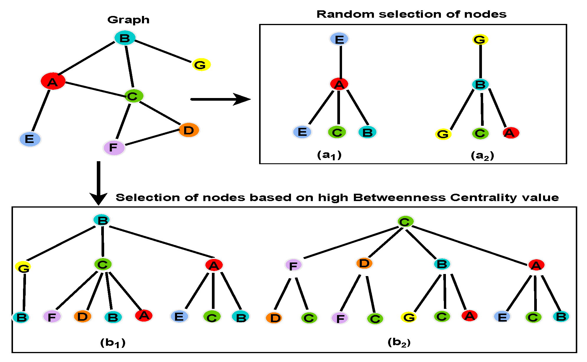
Let us consider an example to verify this. Figure 4 illustrates the computational graphs corresponding to a node for the graph defined in the first subfigure of Figure 4. Suppose that for this graph G, the size of the training set is 2. Consider the two subsets A (random selection) and A (proposed selection) as:
A = E , G
A = B , C
Thus, extending the computational graphs of the selected training nodes in A to the neighbors up to path length 2 (fixed size z path length), the node coverage of A :
A = A , B , C , E , G
On the other hand, node coverage for A using the training nodes B and C is:
A = A , B , C , D , E , F , G
This small illustration shows that A has a larger node coverage compared to A’. Moreover, each node a i A is a feature matrix row associated with it as an A V , and for each node v i V , there is a feature vector x j X such that 1 < i < n , and 1 < j < m , ∀ i , m > 1 . Each node of A” delivers its feature vector to as many nodes as it can reach within the defined constrained path length z. This implies a higher neighborhood contribution compared to the nodes of the subset A . In this way, we finally have a greater availability of feature vectors and labeling information for training the GAT model. From this, we can deduce that the training efficiency of the model (GAT /GCN) is higher when the selection of the training nodes is based on the betweenness centrality model, and therefore, the assignment function (class prediction) obtained for each node in V will eventually be close to the optimal assignment function L.
Next, we will try to show that probability of selection of this subset of nodes ( A ) randomly is near equal to zero.
Definition 1. 
The probability that the GAT model (random selection of training nodes by default) selects the same subset of nodes approaches zero.
In GAT, the selection of training nodes is conducted randomly from the set of available nodes. In our proposed method, on the other hand, these training nodes are selected based on their betweenness centrality scores. Thus, the subset A contains the best w central nodes with the highest betweenness centrality such that w < n , where ‘n’ is the total number of nodes in the network. This is due to the fact that in GCN we have very few nodes that can be used for training, since no information (features and labels) is available. The number of ways to select a subset of length w (subset of w nodes) is given as n C w . Our goal is to find the probability of choosing the subset A from these n C w subsets. Thus, let us consider an event Q as: Selection of the subset A of the set V, where V is the set of all vertices of the graph and | V | = n . The probability of this event will be:
P ( Q ) = 1 / n C w
Assuming that 60 % of the data is used for the training, we then obtain w = 3 n / 5 . Thus:
P ( Q ) = 1 / n C 3 n / 5
If we solve the problem, we obtain P ( Q ) 0 . To check it empirically, if the value of n = 10 4 , then the probability of the event Q according to the above expression is given as follows:
P ( Q ) = 1 / 10 4 C 6000
P ( Q ) = ( 2.68 e 20065 × 1.82 e 12673 ) / 2.84 e 35679
To make the further solution, we have that:
P ( Q ) 1 / e 2921
The value is then calculated as: e 2.73 . Moreover, we have obtained that ( 2.73 ) 2921 > > ( 2.73 ) 5 . Thus, we finally have
P ( Q ) 1 / ( 2.73 ) 5 0
So we can show that the probability that the subset A is chosen at random goes to zero.
Based on the above justifications, we could show that the selection of training nodes based on betweenness centrality improves the efficiency of the GAT model. Therefore, the model will have better classification accuracy than the traditional GAT model where the selection of training nodes is random. Moreover, we found that the probability of selecting all training nodes with the best centrality values is very low (approximately zero). This justifies that this type of selection is almost impossible when the selection of nodes is random. Thus, we could finally justify the efficiency of the proposed model (Bet-GAT) to GAT.

3.3. Proposed Framework

In the proposed framework, we perform the following steps for building a graph neural network model based on betweenness centrality.
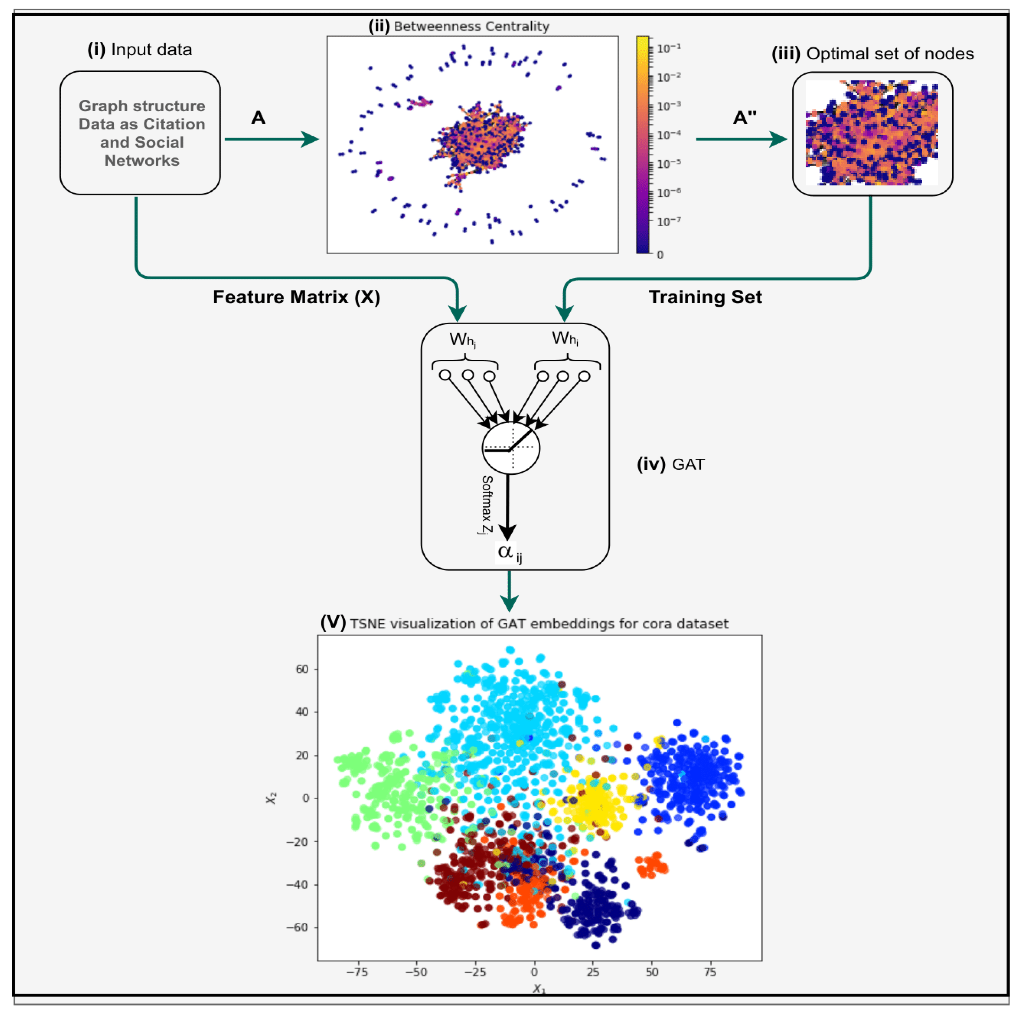
Step (i): We consider data that can be represented in terms of a graph structure (such as citation networks) as input. The set of nodes (A) and the feature matrix (X) of the underlying graph serve as input.
Step (ii): After the input, the betweenness centrality (Bet) is calculated for all nodes using k Equation (11).
Step (iii): Nodes are selected for the training based on betweenness centrality values. Preference is given to nodes with high betweenness centrality values. A subset of nodes (generally top 60 % nodes in terms of betweenness centrality value) are selected for the training.
Step (iv): The chosen training set nodes along with the feature matrix(X) are given to the Graph Attention Network (GAT) for training.
Step (v): Finally, we obtain the classification of nodes as output. In addition, we display the visualization of GAT embeddings for the underlying dataset as t-distributed stochastic neighbour embedding (TSNE).
We consider the Cora citation network to explain the whole process. The Cora dataset includes 2708 scientific publications classified into one of seven classes. In this dataset, the nodes and edges represent documents and citation links, respectively. This dataset is in the form of a set of nodes (A) and a feature matrix (X). Equation (10) is used to represent the betweenness centrality (Bet) of each node from smallest (blue) to largest (yellow) (as in Figure 5). Here, the set of nodes A is divided into two subsets A′ and A″. The subset A” is the set of nodes selected for training (with high values for centrality, i.e., A A ). For further training, we select the set of nodes with the feature matrix GAT Veličković, P. et al. [29]. Then, we use ELU (exponential linear unit) [40] followed by Softmax activation. Lastly, the result is shown as t-distributed stochastic neighbor embedding (TSNE) visualization of GAT embedding for the Cora dataset. Here, each color represents a unique class (category) of the Cora dataset. The dataset has 7 classes and hence, 7 different colors are visible in the TSNE.

3.4. Algorithmic Description of the Problem

To demonstrate the execution of the idea, we use Stellar Graph library [41], which defines the GCN model for a graph. In addition, the graph library NetworkX [42] is used to capture the structural information of the network. The process of node classification was defined in terms of an algorithmic procedure (see Algorithm 1).
The dataset has the form of a graph where the nodes correspond to a data point containing a feature vector. The relationships between the nodes (data points) are represented by edges. These two pieces of information are provided as input to the model. These data are divided into: training data, validation data, and test data. Here, the nodes of the training data are selected based on the centrality measure function (nx.betweenness()) defined by the NetworkX Python library (nx.betweenness()). In addition, the Stellar graph library defines a function FullBatchnode Generator() to define the neural network (NN) for the nodes of the graph. The defined NN generally consists of an input layer, a hidden layer, and an output layer. The number of hidden layers is user-defined and is best determined by experimental simulation runs. In the output layer, the function Softmax is applied to the output obtained from the last hidden layer. Here, the final output is equal to the number of classes to be predicted. The hidden layers have a ReLU (Rectified Linear Unit) activation function with a hidden layer size on the order of 16 × 16 . However, the size of the kernel varies depending on the size of the network. Other parameters of the network, such as the learning rate, are set to 0.01 , with Adam Optimizer and Cross Entropy as loss functions. The Failure Rate for each layer ranges from 0.2–0.5. However, all of these parameter settings are user-dependent and vary slightly in terms of task performance improvement.
Algorithm 1 Pseudocode of Bet-GAT(A, X).
Input: A is the edge list of the network; X is the feature vector matrix corresponding to the dataset containing node labels.
Output: Classification of nodes for the given network.
 dataset = sg.dataset();                         ▹ Loading dataset
 centrality = nx.getcentrality(A);                     ▹ Get centrality
 nodelabels = extractlabels(X);        ▹ Extracting labels from Feature Vector matrix
 nodesubjects = merge (A.nodes, nodelabels);       ▹ Combined node ids with labels
for each node in nodesubjects, centrality do
   nodesubjects1 = merge(nodesubjects, centrality);
   nodesubjects1 = sortbycentrality(nodesubjects1);
end for
for i in range(trainsize) do
   trainset[i] = nodesubjects[i];
end for
for i in range(validationsize) and not in trainset do
   validationset[i] = nodesubjects[i];
end for
for i in range(testsetsize) and not in trainset do
   testset[i] = nodesubjects[i];
end for
 trainset = encode(trainset);                        ▹ One hot encoding
 validationset = encode(validationset);                   ▹ One hot encoding
 testset = encode(testset);                         ▹ One hot encoding
 GAT = GAT (layersizes = [128, 32], activations = [“relu”, “relu”], generator = generator, dropout = 0.5, attention head = 32);                   ▹ Defining GAT layer
 predictions = layers.Dense(units = trainsettargets, activation = “softmax”)(X); ▹ Defining Prediction layer
 model = Model(inputs = X, outputs = predictions);
                                 ▹ Defining the model
 model.compile (optimizer = Adam(learningrate = 0.0001), loss = categoricalcrossentropy, metrics = [“accurracy”]);
 model.fit( trainset, epochs, validationdata, callbacks = till stopping criteria); ▹ Performing Training

3.5. Dataset Description

We use five benchmark datasets (see Table 1) to evaluate the performance of the proposed model. The details of the datasets are as follows.
  • Citation networks: In citation networks, the nodes and edges represent documents and citation links (undirected), respectively. We consider following three datasets in the citation networks.
    (1). Cora: The Cora dataset comprises 2708 scientific publications. Each publication is further classified into 1 of 7 classes.
    (2). Citeseer: The Citeseer dataset contains 3312 scientific publications. Each publication is categorised into 1 of 6 classes.
    (3). PubMed: The PubMed dataset contains 19,717 scientific publications. Each publication is further classified into one of three classes.
  • Wikipedia-based [43]: Wiki-CS is a relatively new dataset from Wikipedia. The nodes and edges represent computer science articles and hyperlinks, respectively. The dataset contains 11,701 computer science articles which are categorised into 10 classes.
  • AMZ computers [44]: AMZ Computers is an Amazon co-purchase graph. The nodes and edges of this graph represent items and co-purchased relation respectively. The dataset contains 13,752 products which are categorised into 10 classes.

4. Results and Analysis

In this section, the effectiveness of the model’s performance is demonstrated experimentally. A comparative analysis of the behavioral aspects of the proposed model with the traditional GCN model is performed. We also present experimental results obtained with the Bet-GAT model for three datasets. We also compare our results with other state-of-the-art methods.

4.1. A Comparative Analysis: GCN vs. GCN with Betweenness Centrality

In this subsection, we compare the behavior of our model (GCN with betweenness centrality) with the GCN model. We consider the Zachary Karate Club network and analyze the node embeddings generated by the two models for this network. For this node embedding process, we consider Equations (1), (4), and (5) as defined in Section 2.1.
Figure 6a shows the network of the Zachary Karate club, which consists of two classes. In these two classes, there are 34 nodes connected by 78 unweighted and undirected edges. Using this well-known network, we analyze the proposed idea (GCN with betweenness centrality) for classifying nodes in graphs. To empirically test our idea, we train the GCN model by randomly initializing the transformation matrices into the Zachary Karate Club network [45]. Then, we train the GCN with the betweenness centrality model based on selecting the training nodes with high betweenness centrality values. We also draw the node embeddings. When we compare the node embeddings of both models, we find that GCN performs well, but GCN performs better with the betweenness centrality model. Figure 6b,c show the node embeddings of GCN and GCN with the betweenness centrality model, respectively. Through observations and a comparative study of both embeddings, we show the correctness of our claim that GCN performs better with the betweenness centrality.
Our idea provides better performance in terms of dispersion and proximity of nodes, while the traditional GCN may consider nodes that do not contribute much to the functions (such as leaf nodes or nodes with lower importance). The main reason for the better performance of the GCN with the betweenness centrality is the consideration of nodes with high betweenness centrality over random nodes in GCN. Nodes with high betweenness centrality appear in many shortest path node pairs and therefore tend to contribute more to the features during training.

4.2. Experimental Results

The results of our proposed model are summarized in Table 2. In terms of performance (accuracy), our proposed Bet-GAT model (betweenness centrality with graph attention network) is in line with the state of the art for the five benchmark networks: Cora, Citeseer PubMed, Wiki-CS, and AMZ Computers.
For node classification, methods, such as multilayer perceptron (MLP) and logistic regression (LR), consider only node features. On the other hand, a method such as the label propagation algorithm (LPA) focuses only on graph structure [46]. Overall, these three methods do not fully utilize the underlying network (dataset) (either in terms of structural properties or node features). This is the main reason for the lower accuracy of these methods (see Table 2). In the case of GCN [2] and GAT methods [29], we find that they provide better results in different citation networks compared to the previously discussed methods. We have already justified why our proposed method performs better than the traditional GCN/GAT model. In other methods, such as jumping knowledge networks (JK-Net) [47] and GCN- label propagation algorithm (GCN-LPA) [28], we find that JK-Net works on subgraphs with distinct local structures generated based on random walks. JK-Net is a strong foundation for Cora, but it does not provide the same for other datasets. The GCN-LPA model allows simultaneous learning of transformation matrices and edge weights. Therefore, it provides better performance than the traditional GCN. With our proposed GAT implementation, we achieve a classification accuracy of 89.15 % for Cora, 81 % for Citeseer, and 87.5 % for PubMed. These results exceed the classification accuracy of the other state-of-the-art-based GCN implementations [28] (see Table 2).
Our proposed model focuses on the structural properties of the underlying graph for feature generation and prediction. Bet-GAT architectural hyperparameters were fine-tuned for the Cora, Citeseer, and PubMed datasets. We consider the ratio of 6:3:1 for the partitioning of the training set, the validation set, and the test set. We use a two-layer GAT model. For the first layer, we use 32 attention heads, each computing 128 hidden node features. The label classification result is provided by the second layer. Then, we use ELU (exponential linear unit) [40] followed by Softmax activation. We also apply dropout = 0.5 for both layers. During training, we apply L2 regularization with a learning rate of 0.0005 . The weight of each edge is treated as a free variable during training. We train our model for 1000 epochs using Adam [48]. The same hyperparameters are applied to all three datasets
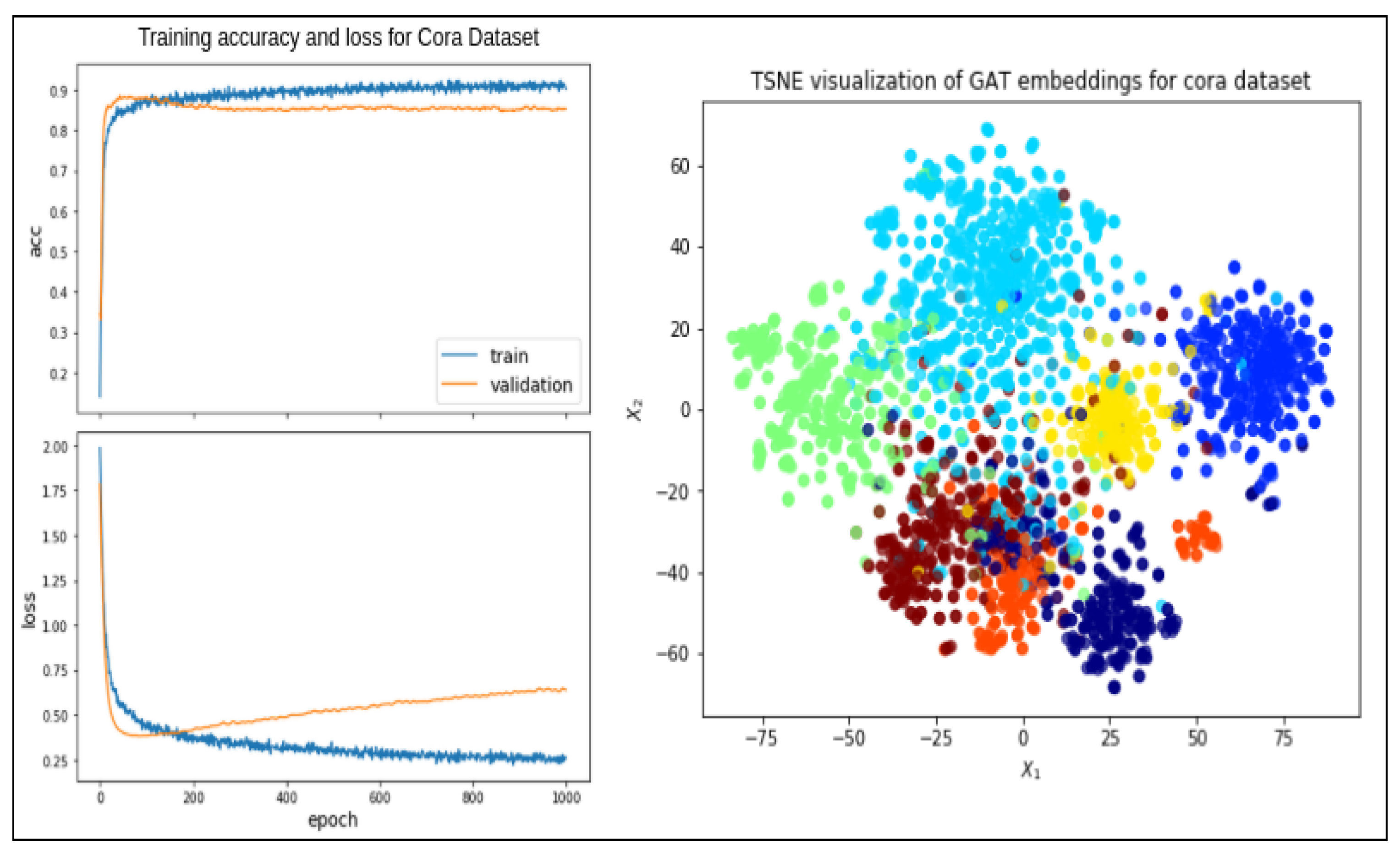
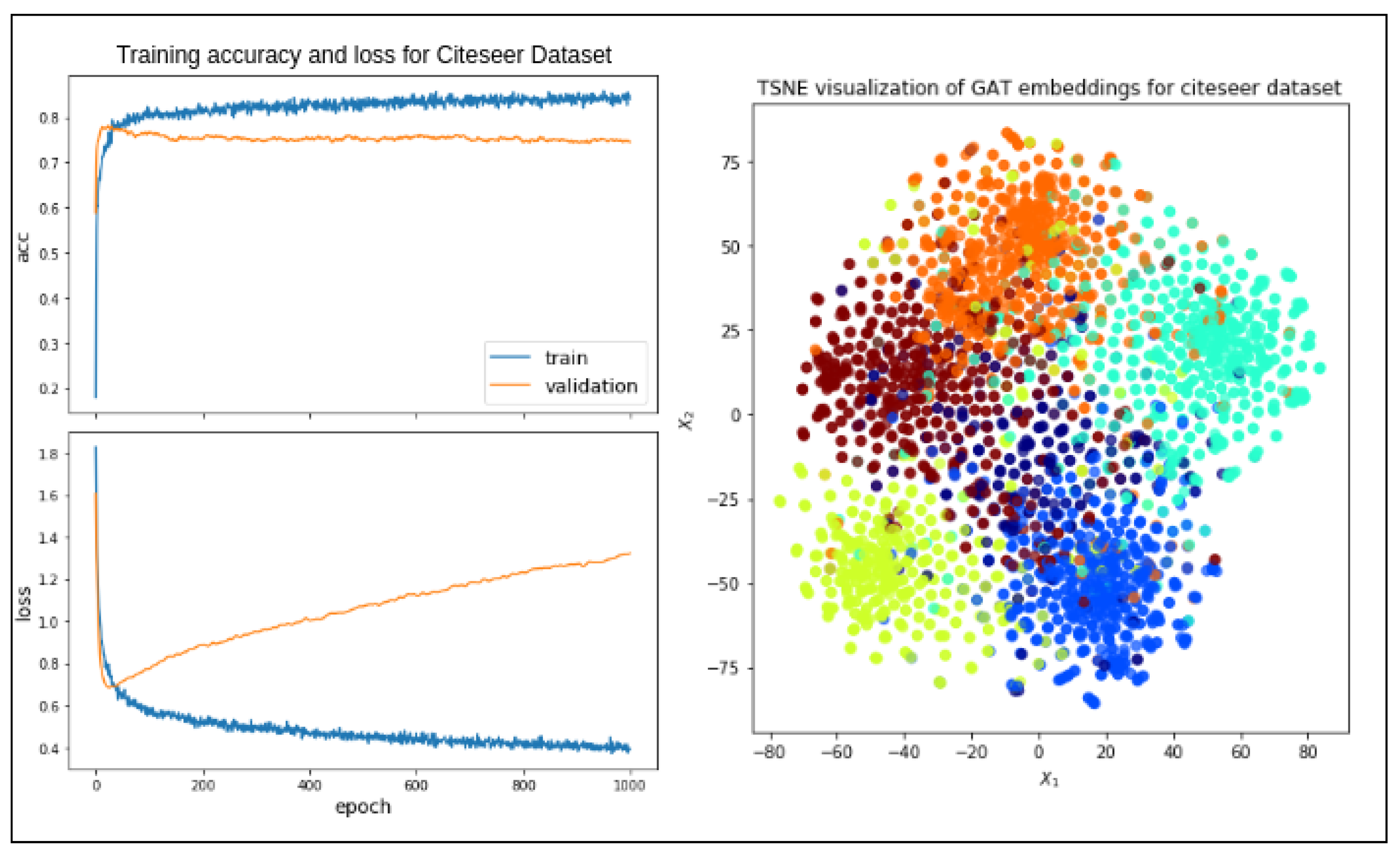
In Figure 7, Figure 8 and Figure 9, we have shown the graphical representations of the accuracy and loss curves for the Cora, Citeseer, and PubMed citation networks. The graphical representations of the datasets in the form of TSNE embeddings show clusters of different classes (seven, six, and three clusters for Cora, Citeseer, and PubMed, respectively). Accuracy and loss curves are plotted for the training and validation phases. For the graphs, the epochs are shown on the x-axis, and the accuracy and loss are shown on the y-axis. We obtain 89.15 % accuracy with loss 0.3712 for CORA, 79.00 % accuracy with loss 0.4143 for Citeseer, and 81.00 % accuracy with loss 0.3400 for PubMed.
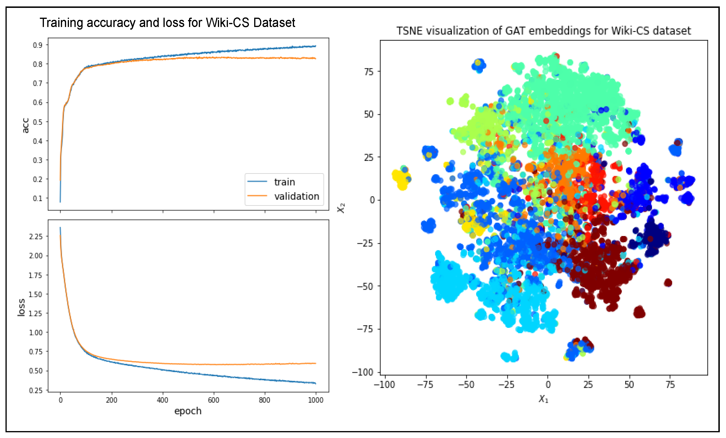
In Figure 10, we show the accuracy and loss curves for the Wiki-CS dataset. The corresponding TSNE GAT embeddings (graphical representation) show clusters for the ten different classes. For the training and validation phases, the accuracy and loss curves are plotted (epochs are plotted on the x-axis and accuracy and loss on the y-axis). We obtain an accuracy of 85.073 % with a loss of 0.4639 for Wiki-CS.
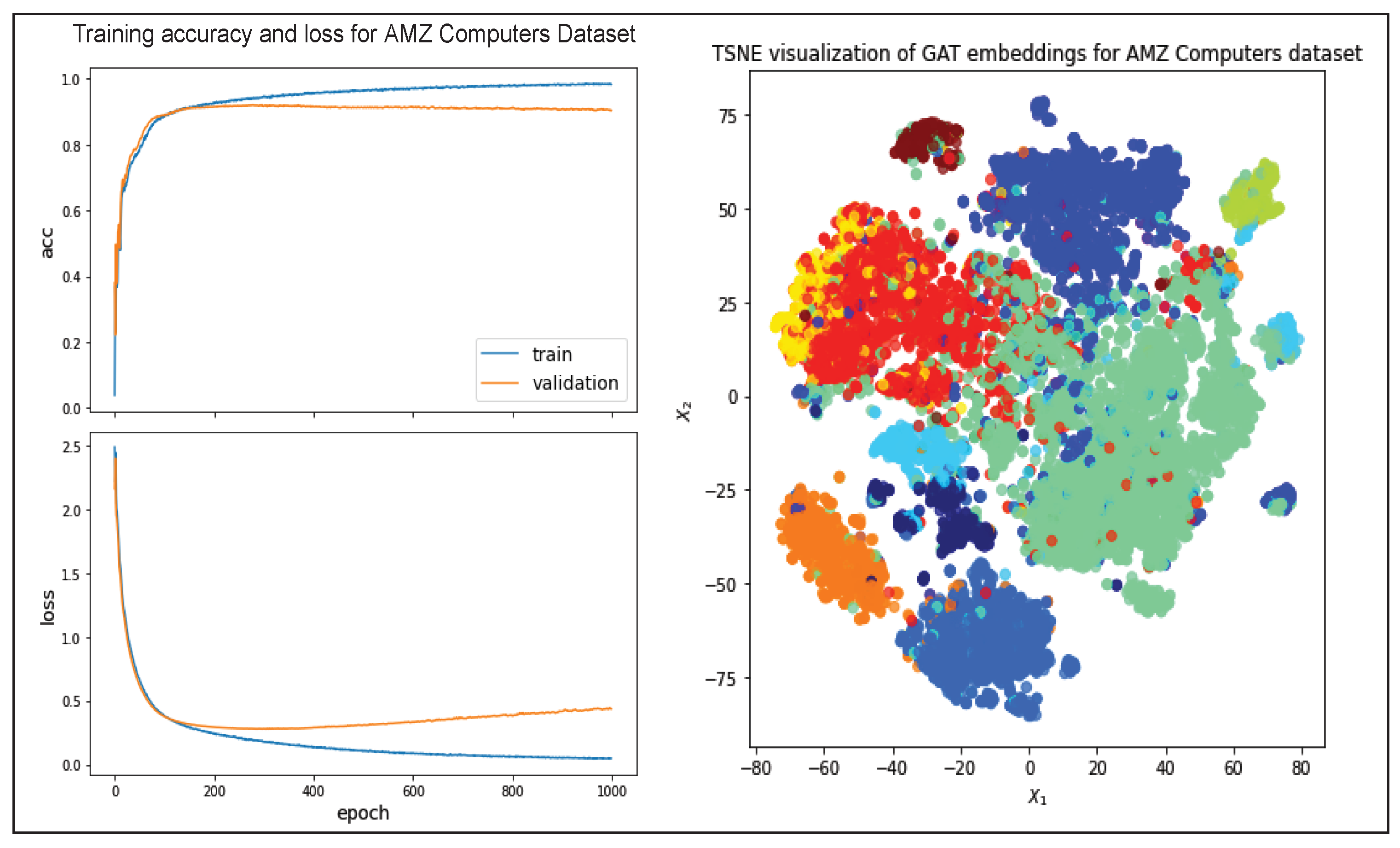
Finally, in Figure 11 we have presented the graphs of accuracy and training loss for the AMZ computers. The corresponding TSNE GAT embeddings show clusters for its three classes. For training and validation, the accuracy and loss graphs are plotted (x-axis shows epochs and y-axis shows accuracy and loss). We obtain an accuracy of 91.05 % for Amazon with a loss of 0.2641 . For verification of our proposed model, we calculate the generalization error that refers to the test error of the model, which indicates how well a model generalizes to the unseen data. We experimentally analyzed the training and test errors for the mentioned datasets and observed that even though test error tends to be greater than training error loss, the difference is not very significant. In the case of Cora, the training error and test error loss values are 0.3712 and 0.25 , respectively, with test accuracy being 89.15 % . For Citeseer, the training error and test error loss values are 0.4143 and 1.2 , respectively, with test accuracy being 79 % . In the case of Citeseer, the training to test error loss is high which accounts for low accuracy of the model over this dataset as compared to CORA. In addition, it can be observed that the loss value difference is not huge and due to which model performs well to classify the unseen node labels. For CORA, the base GAT model has training and test loss values ranging above 0.5 or more attaining an accuracy of around 85 % . So, here the loss increases, and also the difference between the training to test error loss is marginally high. With respect to the model complexity, our proposed model just adds up a step of identifying the nodes based on the betweenness centrality which is a preprocessing step and a one time evaluation task for the nodes of the graph. So, it does not add up to the overall complexity of the model for predicting the node labels. Thus, Bet-GAT has the same model complexity as the base GAT model and a minimized generalization error which makes it a suitable choice to prefer.
The F1 score is an indicative measure of the accuracy of the model. The F1 scores (calculated using different methods) for the five benchmark datasets were compared with the other state-of-the-art methods. The score gained through the training are as follows: Cora ( 87 % ), Citeseer ( 84 % ), PubMed ( 84 % ), Wiki-CS ( 86 % ), and AMZ computers ( 95 % ) (see Table 3).

5. Conclusions

We propose an efficient graph-attention-based semi-supervised classification method (Bet-GAT) where training nodes are selected based on betweenness centrality. The model essentially exploits the fact that GNN-based models rely on aggregation of neighborhood information. In a graph network, the structurally well-positioned nodes ensure good aggregation of information. This key idea is used to train the model. The classification results obtained on the five benchmark datasets (Cora, Citeseer, PubMed, Wiki- CS, and AMZ Computers) show that the prediction accuracy of the proposed model is high. We also present a comparative analysis of the performance of the proposed model with current models and algorithms for semi-supervised node classification. The approach can be further extended to explore the combination of centrality measures (betweenness-closeness, betweenness-degree, etc.) for training node selection.

Author Contributions

Methodology, A.K.V. and M.J.; Validation, J.C.-W.L.; Formal analysis, R.S.; Investigation, M.J.; Writing—original draft, A.K.V.; Writing—review & editing, J.C.-W.L.; Project administration, V.B. All authors have read and agreed to the published version of the manuscript.

Funding

This research received no external funding.

Institutional Review Board Statement

Not applicable.

Informed Consent Statement

Not applicable.

Data Availability Statement

Not applicable.

Conflicts of Interest

The authors declare no conflict of interest.

References

  1. Wu, Z.; Pan, S.; Chen, F.; Long, G.; Zhang, C.; Philip, S.Y. A comprehensive survey on graph neural networks. IEEE Trans. Neural Netw. Learn. Syst. 2020, 32, 4–24. [Google Scholar] [CrossRef] [PubMed] [Green Version]
  2. Kipf, T.N.; Welling, M. Semi-supervised classification with graph convolutional networks. In Proceedings of the International Conference on Learning Representations, Toulon, France, 24–26 April 2017. [Google Scholar]
  3. Kumar, A.; Singh, S.S.; Singh, K.; Biswas, B. Link prediction techniques, applications, and performance: A survey. Phys. Stat. Mech. Appl. 2020, 553, 124289. [Google Scholar] [CrossRef]
  4. Kriege, N.M.; Johansson, F.D.; Morris, C. A survey on graph kernels. Appl. Netw. Sci. 2020, 5, 1–42. [Google Scholar] [CrossRef] [Green Version]
  5. Derrow-Pinion, A.; She, J.; Wong, D.; Lange, O.; Hester, T.; Perez, L.; Nunkesser, M.; Lee, S.; Guo, X.; Wiltshire, B.; et al. Eta prediction with graph neural networks in google maps. In Proceedings of the 30th ACM International Conference on Information & Knowledge Management, Queensland, Australia, 1–5 November 2021; pp. 3767–3776. [Google Scholar]
  6. Zaki, N.; Singh, H.; Mohamed, E.A. Identifying protein complexes in protein-protein interaction data using graph convolutional network. IEEE Access 2021, 9, 123717–123726. [Google Scholar] [CrossRef]
  7. Cao, P.; Zhu, Z.; Wang, Z.; Zhu, Y.; Niu, Q. Applications of graph convolutional networks in computer vision. Neural Comput. Appl. 2022, 34, 13387–13405. [Google Scholar] [CrossRef]
  8. Vashishth, S.; Yadati, N.; Talukdar, P. Graph-based deep learning in natural language processing. In Proceedings of the 7th ACM IKDD CoDS and 25th COMAD, Hyderabad, India, 5–7 January 2020; pp. 371–372. [Google Scholar]
  9. Meng, Y.; Wei, M.; Gao, D.; Zhao, Y.; Yang, X.; Huang, X.; Zheng, Y. CNN-GCN aggregation enabled boundary regression for biomedical image segmentation. In Proceedings of the International Conference on Medical Image Computing and Computer-Assisted Intervention, Lima, Peru, 4–8 October 2020; pp. 352–362. [Google Scholar]
  10. Wang, B.; Shen, G.; Li, D.; Hao, J.; Liu, W.; Huang, Y.; Wu, H.; Lin, Y.; Chen, G.; Heng, P.A. LHNN: Lattice Hypergraph Neural Network for VLSI Congestion Prediction. arXiv 2022, arXiv:2203.12831. [Google Scholar]
  11. Das, K.; Samanta, S.; Pal, M. Study on centrality measures in social networks: A survey. Soc. Netw. Anal. Min. 2018, 8, 13. [Google Scholar] [CrossRef]
  12. Derr, T.; Ma, Y.; Fan, W.; Liu, X.; Aggarwal, C.; Tang, J. Epidemic graph convolutional network. In Proceedings of the 13th International Conference on Web Search and Data Mining, Houston, TX, USA, 10–13 July 2020; pp. 160–168. [Google Scholar]
  13. Xu, B.; Shen, H.; Cao, Q.; Qiu, Y.; Cheng, X. Graph Wavelet Neural Network. In Proceedings of the International Conference on Learning Representations, Vancouver, BC, Canada, 30 April–3 May 2018. [Google Scholar]
  14. Abu-El-Haija, S.; Perozzi, B.; Kapoor, A.; Alipourfard, N.; Lerman, K.; Harutyunyan, H.; Ver Steeg, G.; Galstyan, A. Mixhop: Higher-order graph convolutional architectures via sparsified neighborhood mixing. In Proceedings of the International Conference on Machine Learning, Long Beach, CA, USA, 9–15 June 2019; pp. 21–29. [Google Scholar]
  15. Lu, H.; Huang, S.H.; Ye, T.; Guo, X. Graph star net for generalized multi-task learning. arXiv 2019, arXiv:1906.12330. [Google Scholar]
  16. Ma, J.; Tang, W.; Zhu, J.; Mei, Q. A flexible generative framework for graph-based semi-supervised learning. Adv. Neural Inf. Process. Syst. 2019, 32, 3281–3290. [Google Scholar]
  17. Zügner, D.; Günnemann, S. Certifiable robustness and robust training for graph convolutional networks. In Proceedings of the 25th ACM SIGKDD International Conference on Knowledge Discovery & Data Mining, Anchorage, AK, USA, 4–8 August 2019; pp. 246–256. [Google Scholar]
  18. Lin, G.; Wang, J.; Liao, K.; Zhao, F.; Chen, W. Structure Fusion Based on Graph Convolutional Networks for Node Classification in Citation Networks. Electronics 2020, 9, 432. [Google Scholar] [CrossRef] [Green Version]
  19. Gao, H.; Wang, Z.; Ji, S. Large-scale learnable graph convolutional networks. In Proceedings of the 24th ACM SIGKDD International Conference on Knowledge Discovery & Data Mining, London, UK, 19–23 August 2018; pp. 1416–1424. [Google Scholar]
  20. Luo, Y.; Ji, R.; Guan, T.; Yu, J.; Liu, P.; Yang, Y. Every node counts: Self-ensembling graph convolutional networks for semi-supervised learning. Pattern Recognit. 2020, 106, 107451. [Google Scholar] [CrossRef]
  21. Franceschi, L.; Niepert, M.; Pontil, M.; He, X. Learning discrete structures for graph neural networks. In Proceedings of the International Conference on Machine Learning, Long Beach, CA, USA, 9–15 June 2019; pp. 1972–1982. [Google Scholar]
  22. Zhou, K.; Song, Q.; Huang, X.; Hu, X. Auto-gnn: Neural architecture search of graph neural networks. arXiv 2019, arXiv:1909.03184. [Google Scholar] [CrossRef] [PubMed]
  23. Gao, Y.; Yang, H.; Zhang, P.; Zhou, C.; Hu, Y. Graphnas: Graph neural architecture search with reinforcement learning. arXiv 2019, arXiv:1904.09981. [Google Scholar]
  24. Jiang, B.; Zhang, Z.; Tang, J.; Luo, B. Graph optimized convolutional networks. arXiv 2019, arXiv:1904.11883. [Google Scholar]
  25. Wijesinghe, W.; Wang, Q. DFNets: Spectral CNNs for graphs with feedback-looped filters. Adv. Neural Inf. Process. Syst. 2019, 32, 6009–6020. [Google Scholar]
  26. Dabhi, S.; Parmar, M. NodeNet: A Graph Regularised Neural Network for Node Classification. arXiv 2020, arXiv:2006.09022. [Google Scholar]
  27. Huang, W.; Zhang, T.; Rong, Y.; Huang, J. Adaptive sampling towards fast graph representation learning. Adv. Neural Inf. Process. Syst. 2018, 31, 4563–4572. [Google Scholar]
  28. Wang, H.; Leskovec, J. Unifying graph convolutional neural networks and label propagation. arXiv 2020, arXiv:2002.06755. [Google Scholar]
  29. Veličković, P.; Cucurull, G.; Casanova, A.; Romero, A.; Lio, P.; Bengio, Y. Graph attention networks. arXiv 2017, arXiv:1710.10903. [Google Scholar]
  30. Yu, Z.; Wang, H.; Liu, Y.; Böhm, C.; Shao, J. Community Attention Network for Semi-supervised Node Classification. In Proceedings of the 2020 IEEE International Conference on Data Mining (ICDM), Sorrento, Italy, 17–20 November 2020; pp. 1382–1387. [Google Scholar]
  31. Shanthamallu, U.S.; Thiagarajan, J.J.; Spanias, A. A regularized attention mechanism for graph attention networks. In Proceedings of the ICASSP 2020-2020 IEEE International Conference on Acoustics, Speech and Signal Processing (ICASSP), Barcelona, Spain, 4–8 May 2020; pp. 3372–3376. [Google Scholar]
  32. Wang, G.; Ying, R.; Huang, J.; Leskovec, J. Improving graph attention networks with large margin-based constraints. arXiv 2019, arXiv:1910.11945. [Google Scholar]
  33. Roethlisberger, F.J.; Dickson, W.J. Management and the Worker; Psychology Press: London, UK, 2003; Volume 5. [Google Scholar]
  34. Liu, C.C.; Chen, Y.C.; Tai, S.J.D. A social network analysis on elementary student engagement in the networked creation community. Comput. Educ. 2017, 115, 114–125. [Google Scholar] [CrossRef]
  35. Cohen, E.; Delling, D.; Pajor, T.; Werneck, R.F. Computing classic closeness centrality, at scale. In Proceedings of the Second ACM conference on Online Social Networks, Dublin, Ireland, 1–2 October 2014; pp. 37–50. [Google Scholar]
  36. Boldi, P.; Vigna, S. Axioms for centrality. Internet Math. 2014, 10, 222–262. [Google Scholar] [CrossRef] [Green Version]
  37. Bonacich, P. Some unique properties of eigenvector centrality. Soc. Netw. 2007, 29, 555–564. [Google Scholar] [CrossRef]
  38. Barthelemy, M. Betweenness centrality in large complex networks. Eur. Phys. J. B 2004, 38, 163–168. [Google Scholar] [CrossRef]
  39. Bhardwaj, S.; Niyogi, R.; Milani, A. Performance analysis of an algorithm for computation of betweenness centrality. In Proceedings of the International Conference on Computational Science and Its Applications, Santander, Spain, 20–23 June 2011; pp. 537–546. [Google Scholar]
  40. Clevert, D.A.; Unterthiner, T.; Hochreiter, S. Fast and accurate deep network learning by exponential linear units (elus). arXiv 2015, arXiv:1511.07289. [Google Scholar]
  41. Zhang, Z.; Wang, X.; Zhu, W. Automated Machine Learning on Graphs: A Survey. arXiv 2021, arXiv:2103.00742. [Google Scholar]
  42. Kaur, M.; Kaur, H. Implementation of Enhanced Graph Layout Algorithm for Visualizing Social Network Data using NetworkX Library. Int. J. Adv. Res. Comput. Sci. 2017, 8, 287–292. [Google Scholar]
  43. Mernyei, P.; Cangea, C. Wiki-cs: A wikipedia-based benchmark for graph neural networks. arXiv 2020, arXiv:2007.02901. [Google Scholar]
  44. Shchur, O.; Mumme, M.; Bojchevski, A.; Günnemann, S. Pitfalls of graph neural network evaluation. arXiv 2018, arXiv:1811.05868. [Google Scholar]
  45. Zachary, W.W. An information flow model for conflict and fission in small groups. J. Anthropol. Res. 1977, 33, 452–473. [Google Scholar] [CrossRef]
  46. Zhu, X. Semi-Supervised Learning with Graphs; Carnegie Mellon University: Pittsburgh, PA, USA, 2005. [Google Scholar]
  47. Xu, K.; Li, C.; Tian, Y.; Sonobe, T.; Kawarabayashi, K.i.; Jegelka, S. Representation learning on graphs with jumping knowledge networks. In Proceedings of the International Conference on Machine Learning, Stockholm Sweden, 10–15 July 2018; pp. 5453–5462. [Google Scholar]
  48. Kingma, D.P.; Ba, J. Adam: A method for stochastic optimization. arXiv 2014, arXiv:1412.6980. [Google Scholar]
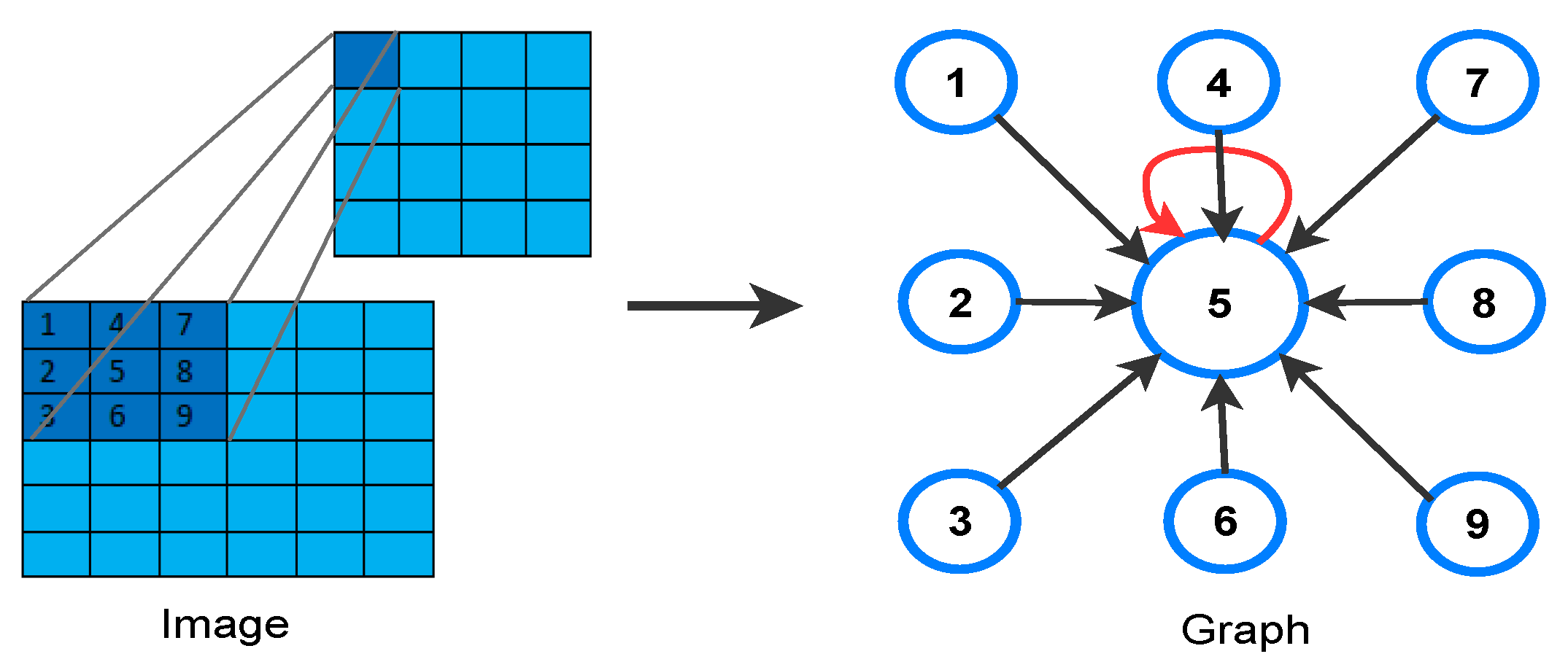
Figure 1. Convolutional operational strategies for regular grid structures and irregular graph structures.
Applsci 13 00847 g001
Figure 2. Semi-supervised node classification through a GCN model.
Applsci 13 00847 g002
Figure 3. Instance of a path graph ( P 5 ) with centrality scores based on importance.
Applsci 13 00847 g003
Figure 4. Node selection: a1, a2 (traditional random selection) vs b1, b2 (proposed selection).
Applsci 13 00847 g004
Figure 5. Diagrammatic representation of node sampling based on betweenness centrality.
Applsci 13 00847 g005
Figure 6. Node embedding of GCN and GCN with betweenness centrality.
Applsci 13 00847 g006
Figure 7. Graphical representation for Cora dataset.
Applsci 13 00847 g007
Figure 8. Graphical representation for Citeseer dataset.
Applsci 13 00847 g008
Figure 9. Graphical representation for PubMed dataset.
Applsci 13 00847 g009
Figure 10. Graphical representation for Wiki-CS dataset.
Applsci 13 00847 g010
Figure 11. Graphical representation for AMZ Computers dataset.
Applsci 13 00847 g011
Table 1. Datasets description.
DatasetsNodesEdgesClassesFeaturesType
Cora2708542971433Citation network
Citeseer3312473263703Citation network
PubMed19,71744,3383500Citation network
Wiki-CS11,7014,31,72610767Wikipedia-based
AMZ Computers13,7524,91,72210300Amazon Computers
Table 2. Experimental results.
MethodCoraCiteseerPubMedWiki-CSAMZ Computers
MLP64.6 ± 1.762.0 ± 1.885.9 ± 0.373.17 ± 0.1944.9 ± 5.8
LR77.3 ± 1.871.2 ± 1.886.0 ± 0.6--
LPA(2005) [46]85.3 ± 0.970.0 ± 1.782.6 ± 0.6--
GCN(2017) [2]88.2 ± 0.877.3 ± 1.587.2 ± 0.479.07 ± 0.1082.6 ± 2.4
GAT(2018) [29]87.7 ± 0.376.2 ± 0.986.9 ± 0.579.63 ± 0.1078.0 ± 1.9
JK-Net(2018) [47]89.1 ± 1.278.3 ± 0.985.8 ± 1.1--
GCN-LPA(2020) [28]88.5 ± 1.578.7 ± 0.687.8 ± 0.6--
Bet-GAT(Proposed)89.15 ± 1.579.0 ± 0.387.5 ± 0.585.73 ± 0.391.05 ± 1.3
Table 3. F1 Score.
Table 3. F1 Score.
MethodCoraCiteseerPubMedWiki-CSAMZ Computers
GCN(2017) [2]0.830.710.780.780.84
GAT(2018) [29]0.840.700.780.770.88
JK-Net(2018) [47]0.820.690.77--
Bet-GAT(Proposed)0.870.840.840.860.95
Disclaimer/Publisher’s Note: The statements, opinions and data contained in all publications are solely those of the individual author(s) and contributor(s) and not of MDPI and/or the editor(s). MDPI and/or the editor(s) disclaim responsibility for any injury to people or property resulting from any ideas, methods, instructions or products referred to in the content.