Article

Identifying Synthetic Faces through GAN Inversion and Biometric Traits Analysis

by
Cecilia Pasquini
1,2,*,
Francesco Laiti
3,†,
Davide Lobba
3,†,
Giovanni Ambrosi
3,
Giulia Boato
3,4 and
Francesco De Natale
3,4
1
Fondazione Bruno Kessler, 38123 Povo, Italy
2
Futuro e Conoscenza srl, 00138 Rome, Italy
3
Department of Information Engineering and Computer Science, University of Trento, 38122 Trento, Italy
4
CNIT—Consorzio Nazionale Interuniversitario per le Telecomunicazioni, 43124 Parma, Italy
*
Author to whom correspondence should be addressed.
These authors contributed equally to this work.
Appl. Sci. 2023, 13(2), 816; https://doi.org/10.3390/app13020816
Submission received: 29 November 2022 / Revised: 29 December 2022 / Accepted: 31 December 2022 / Published: 6 January 2023
(This article belongs to the Special Issue On the Role of Synthetic Data in Biometrics)

Abstract

:
In the field of image forensics, notable attention has been recently paid toward the detection of synthetic contents created through Generative Adversarial Networks (GANs), especially face images. This work explores a classification methodology inspired by the inner architecture of typical GANs, where vectors in a low-dimensional latent space are transformed by the generator into meaningful high-dimensional images. In particular, the proposed detector exploits the inversion of the GAN synthesis process: given a face image under investigation, we identify the point in the GAN latent space which more closely reconstructs it; we project the vector back into the image space, and we compare the resulting image with the actual one. Through experimental tests on widely known datasets (including FFHQ, CelebA, LFW, and Caltech), we demonstrate that real faces can be accurately discriminated from GAN-generated ones by properly capturing the facial traits through different feature representations. In particular, features based on facial landmarks fed to a Support Vector Machine consistently yield a global accuracy of above 88% for each dataset. Furthermore, we experimentally prove that the proposed detector is robust concerning routinely applied post-processing operations.

1. Introduction

The creation of synthetic media through artificial intelligence has reached unprecedented levels of realism. Impressive results have been achieved in recent years for the semantic generation and manipulation of audio-visual content in fully or semi-automated fashion, also with multi-domain capabilities (e.g., text-to-image (https://openai.com/dall-e-2/ (accessed on 30 December 2022), text-to-speech).
Great effort has been spent in the generation of synthetic visual data. Video signals are highly powerful carriers in terms of semantics that can be conveyed, but they are still more complex to synthesize and manipulate. In fact, despite the rapidly progressing technology, producing high-quality manipulated videos involving arbitrary subjects and scenes still requires considerable skills and processing time. Instead, the generation of still pictures, and in particular the production of synthetic faces, is currently very easy and accessible to everyone, especially thanks to Generative Adversarial Networks (GANs), which can achieve impressive visual quality with minimal computational requirements [1,2]. Generative models are available online [3,4] to automatically generate or even edit face images; web interfaces (https://thispersondoesnotexist.com/ (accessed on 30 December 2022)) running pre-trained generators are also available, requiring no more than a click to obtain a hyper-realistic fake face. Harmful misuses of this technology have already been observed in the web ecosystem, including the creation of fictitious social media profiles (https://edition.cnn.com/2020/02/28/tech/fake-twitter-candidate-2020/index.html (accessed on 30 December 2022)) and digital identities (https://www.nbcnews.com/tech/security/how-fake-persona-laid-groundwork-hunter-biden-conspiracy-deluge-n1245387 (accessed on 30 December 2022)), thus calling for specialized detection technologies.
Researchers have proposed different techniques to distinguish between real and synthetic faces over the years [5,6,7], and great attention has been devoted over the last few years toward identifying whether an image has been generated through a GAN [8,9,10,11]. Further details about the related works are provided in the next section.
In this paper, we propose a novel detector for GAN-generated images based on the analysis of an image resulting from a GAN inversion process. In practice, given an image under investigation, we project it in the GAN latent space through an inversion process [12], and then back into the image space with a generation process. The resulting image is then compared with the actual one using different similarity metrics. We demonstrate that, as expected, when the process is applied to GAN-generated images, the two images will be extremely close to each other. In contrast, natural images will be approximated with significantly lower accuracy.
Extensive experiments on images coming from different sources have shown that landmark-based metrics are particularly effective in capturing the distinctive traits of synthetic images, which can be learned using shallow classifiers such as SVMs. Furthermore, the obtained detectors are proven to be generally robust to typical post-processing, such as resizing, JPEG compression, and upload/download operations through social media.
The major contributions of the paper can be summarized in the following points:
  • We explicitly use the underlying mechanisms of GAN generators to perform the detection, instead of applying a blind learning procedure;
  • We demonstrate that generative approaches produce structural errors in the reproduction of previously unseen face images, which can be revealed through appropriate sets of features;
  • The proposed technique can be extended to any generator that admits an inversion, thus limiting the need for retraining over large image datasets.
  • We release a data corpus of face images and their reconstructions through the StyleGAN2 inversion, available for research purposes.
The rest of the paper is structured as follows: in Section 2, we summarize the current state of research in the field; in Section 3, we describe the proposed inversion-based detector, providing details on the inversion process, and on the feature extraction and classification process; in Section 4, we define the experimental setup and the datasets used for testing, and we analyze the results under different operating conditions; finally, in Section 5, we draw some conclusions.

2. Related Work

In this section, we provide a short survey of the literature on real-versus-generated image detection, focusing in particular on data-driven methods and on the problem of GAN generation and inversion.

2.1. Data-Driven Detection Methods

In the context of real-versus-generated image detection, several approaches have been proposed. As in many related fields, deep networks have been widely exploited for detection purposes. One possibility is to apply them to characterize handcrafted features, as it happens in [13] for co-occurrence matrices. In addition, their inner behavior regarding neuron activation can be used as a clue to detect anomalies due to a synthetic source [14].
However, the most common approach is to employ fully data-driven methods, typically based on Convolutional Neural Networks (CNN), where the most distinctive features [11] are automatically learned from the data with remarkable results. Although they achieve excellent performance under rather aligned conditions in terms of training and testing distributions, it has been shown that they suffer some shortcomings due to their purely inductive nature [8]. This includes a significant loss of performance when the investigated data have undergone some post-processing, perhaps unseen in training, which likely occurs during the digital image life cycle. Data augmentation strategies and the inclusion in the training sets of post-processed samples may help in mitigating these issues [8,15], but they require the simulation of a huge variety of processing pipelines arising in real-world scenarios. Furthermore, deep learning-based approaches are often used as black boxes, thus making it difficult to interpret the inner mechanisms that led to a given decision.
For the above reasons, the performance and reliability of purely data-driven GAN detectors on testing data from uncontrolled settings are hard to predict. On the contrary, principled approaches exploiting the inherent architectural properties of generators represent a promising path to enrich the forensic tools available, and for devising detectors with enhanced generalization and explainability. Accordingly, this work explores the possibility of exploiting the inversion properties of the generator for identifying synthesized data, as explained in the following.

2.2. GAN Image Generation and Inversion

The GANs’ typical inner mechanism entails that (random) vectors lying in a latent space are transformed into semantically meaningful images. This procedure can be also inverted to some extent, by back-projecting an image into a point in the latent space that corresponds to similar content in the image space.
The inversion of generative models has recently drawn strong attention in the computer vision community [12,16]. In this context, an interesting property is that the latent space can be queried and browsed along specific directions corresponding to visual attributes. As a matter of fact, inversion processes are mainly investigated for fast image editing applications. To the best of our knowledge, the only work that exploits inversion properties for inferring information on the image source is [17]. However, in that case, the authors analyze synthetic images only, with the goal of identifying the correct generator among a set of candidates. Moreover, a single distance-based indicator is used, and earlier, less compelling GANs are considered in the experimental analysis.
In our work, we analyze the outcome of the GAN inversion process, which given an image under investigation, finds the point in the GAN latent space that leads to the closest possible generated output in the image domain [12]. We expect that the application of this kind of process to images synthesized by that generator will produce a point in the latent space that leads to an equal or highly similar image, given that such a point exists for sure. On the contrary, the inversion process applied to natural images can only provide a latent vector that is associated with some approximation of the image, according to the considered generative model.
The proposed detector was tested on the widely known and highly realistic StyleGAN2 face generator [4], among the best-performing GAN image synthesizers currently available. The images under investigation are compared to their closest reconstruction obtained through the inversion process available in StyleGAN2, and their biometric facial traits are encoded through different face representations (including deep embeddings and landmark-based features) and learned by conventional classifiers such as SVMs. Conceptually, our work shares similarities with differential morphing detection pipelines, as in [18,19], where face image pairs containing authentic or morphed faces in biometric verification scenarios need to be distinguished, thus also requiring the characterization of subtle differences in facial traits. The use of handcrafted features and lightweight classifiers for detecting synthetic images has also been explored in [20], which however, did not include semantic features. The use of semantic cues for the detection of GAN-generated images has been explored and advocated by several works [21,22,23,24] but, in those cases, semantic artifacts are characterized in a post hoc analysis, thus not relying on the architecture of the generator.

3. Inversion-Based Detection

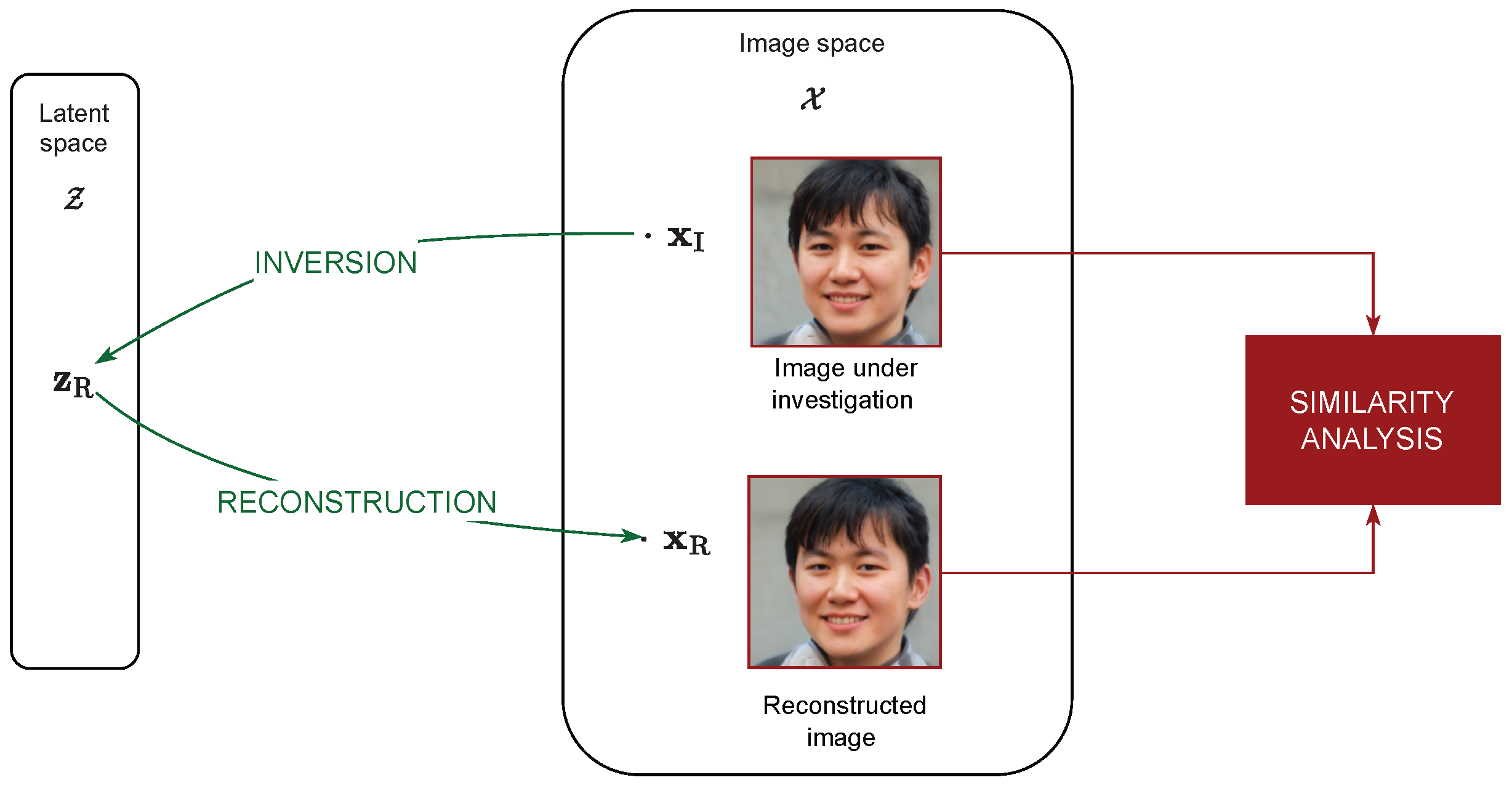
The key idea of the devised forensic strategy is to discriminate between real and GAN-synthesized face images by retro-projecting the image under analysis into the GAN latent space, synthesizing the image associated with the relevant point in the latent space, and comparing the generated image with the actual one.
This concept is represented in Figure 1. We start from an input image under investigation x I (the picture on top of image space), and we feed it into a GAN inversion process to obtain the corresponding point z R in the GAN latent space. We then run the GAN generator to produce a reconstructed version x R of the original image, associated with z R (bottom image in the image space). At this point, we have two copies of the image under analysis, the original and the reconstructed one, and we want to compare them to measure their similarity: the greater the similarity, the higher the probability that the image is GAN-generated. In fact, if the image under analysis comes from this generator, independently of the fact that it was part of the training set or not, a point in the latent space should exist that closely generates the same image. This is not true in the case of a real image, for which that point, in general, will not exist, and the inversion will just provide a more or less accurate approximation but not a perfect reconstruction. Indeed, in practice, we will never obtain a pointwise-equal image due to the limited accuracy of the inversion process, but nevertheless, we expect that GAN-generated images will much more closely match the target than real images.
Thus, properly comparing x I and x R is an important part of the process, as the differences among the two images cannot be just modeled as random noise. For this reason, we jointly perform two types of analysis: one based on standard image similarity measures, and the other on more specific face similarity features, and we analyze the relevant performances.
In the following sub-sections, we further illustrate the two main processes concerned with the above scheme: the inversion process, and the comparison and classification processes.

3.1. Inversion Process

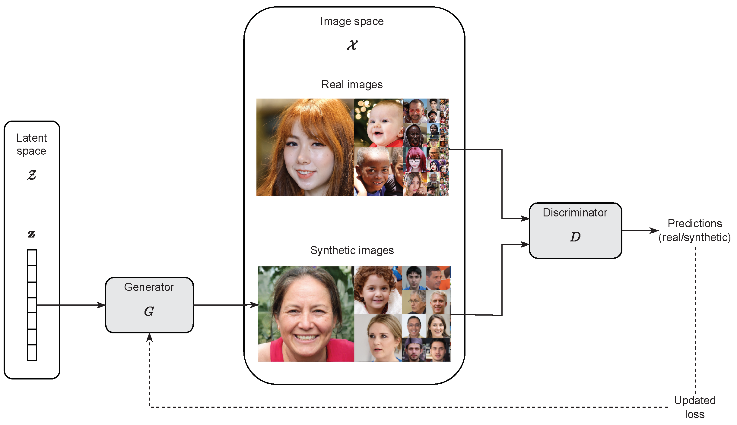
Let us consider the typical GAN architecture, where a generator G and a discriminator D are trained jointly through an adversarial process. The goal of G is to generate synthetic data that resemble real data; the goal of D is to correctly distinguish the synthetic data generated by G and an available corpus of real data [25]. Starting from an initial version of both, the two networks are trained in an alternate manner by competing with each other and progressively improving their performance: the current version of D is fine-tuned on the real samples, and the synthetic ones created by the current version of G; in turn, G is then fine-tuned so as to maximize the classification loss of the updated version of D. At the end of this training process, the distribution of data generated by G is intended to match the distribution of real data, so as to minimize the discrimination capabilities of D.
Generators typically work to transform a randomly drawn vector z Z into an image x = G ( z ) in the image space X . z and Z represent the latent vector and the latent space, respectively, and z encodes information about the appearance of G ( z ) . Figure 2 depicts this mechanism. In other words, during the training process, the mapping G : Z X is learned, and points that are close in the latent space Z are transformed through G into visually similar images in X .
The inversion (or projection) of GANs [12] consists of mapping a certain image under analysis x I back into its corresponding representation in the latent space. Formally, this can be formulated as finding a point z R in Z such that G ( z R ) is as close as possible to x I according to a certain metrics ( · , · ) :
z R = arg min z Z ( G ( z ) , x I )
We denote x R G ( z R ) as the reconstructed version of x I .
In this work, we study the inversion and reconstruction processes by focusing on the case where the generator G is the widely known StyleGAN2 face generator [3], for which the authors also provide a strategy for solving the problem in (1) (see Section 5 of [3]), together with an open source implementation (https://github.com/NVlabs/stylegan2-ada-pytorch (accessed on 30 December 2022)).
Figure 3 reports examples of StyleGAN2 images and their reconstructions.
Therefore, given a face image under analysis x I , possibly coming from a variety of sources, we propose to compare it to its reconstructed version x R . If x I has been actually synthesized by the considered generator G, its reconstruction x R should coincide or be very close to x I , also depending on the effectiveness of the optimization strategy employed to solve the problem in (1). Conversely, when x I is not an output of the generator, the inversion process can only identify the closest reconstruction achievable through G.

3.2. Feature Extraction and Classification Process

After the inversion and reconstruction, we aim at jointly characterizing the visual appearance of x I and x R , with the goal of predicting whether the former has been synthesized through G or not. Thus, in all cases, the objects of our analysis will be images face pairs, which we indicate as being real and synthetic when the related x I is real or synthetic, respectively. In particular, as depicted in Figure 4, we extract a feature representation separately from each image in the pair, thus obtaining F I and F R . Then, a comparison operator between the two is applied, thus obtaining for each pair a single differential feature vector. Those are then used to train a classifier, to automatically characterize the differences resulting from the inversion process.
We employ different feature extractors and comparison rules with the goal of capturing specific biometric traits, resulting in different types of differential feature vectors. In particular, we adopt as feature extractors both deep embeddings and handcrafted features proposed in the literature for automated face analysis tasks, namely:
  • FaceNet embeddings: Proposed in [26], the FaceNet features are the best-performing ones on the LFW face recognition dataset [27] among the deep features selected in the Deepface toolbox (https://github.com/serengil/deepface (accessed on 30 December 2022)). In computing F I and F R , we employ the original 512-dimensional FaceNet version and its compact 128-dimensional variant. In this case, the comparison is simply an element-wise difference in the module.
    We denote as FN 128 R 128 and FN 512 R 512 the two types of differential feature vectors obtained.
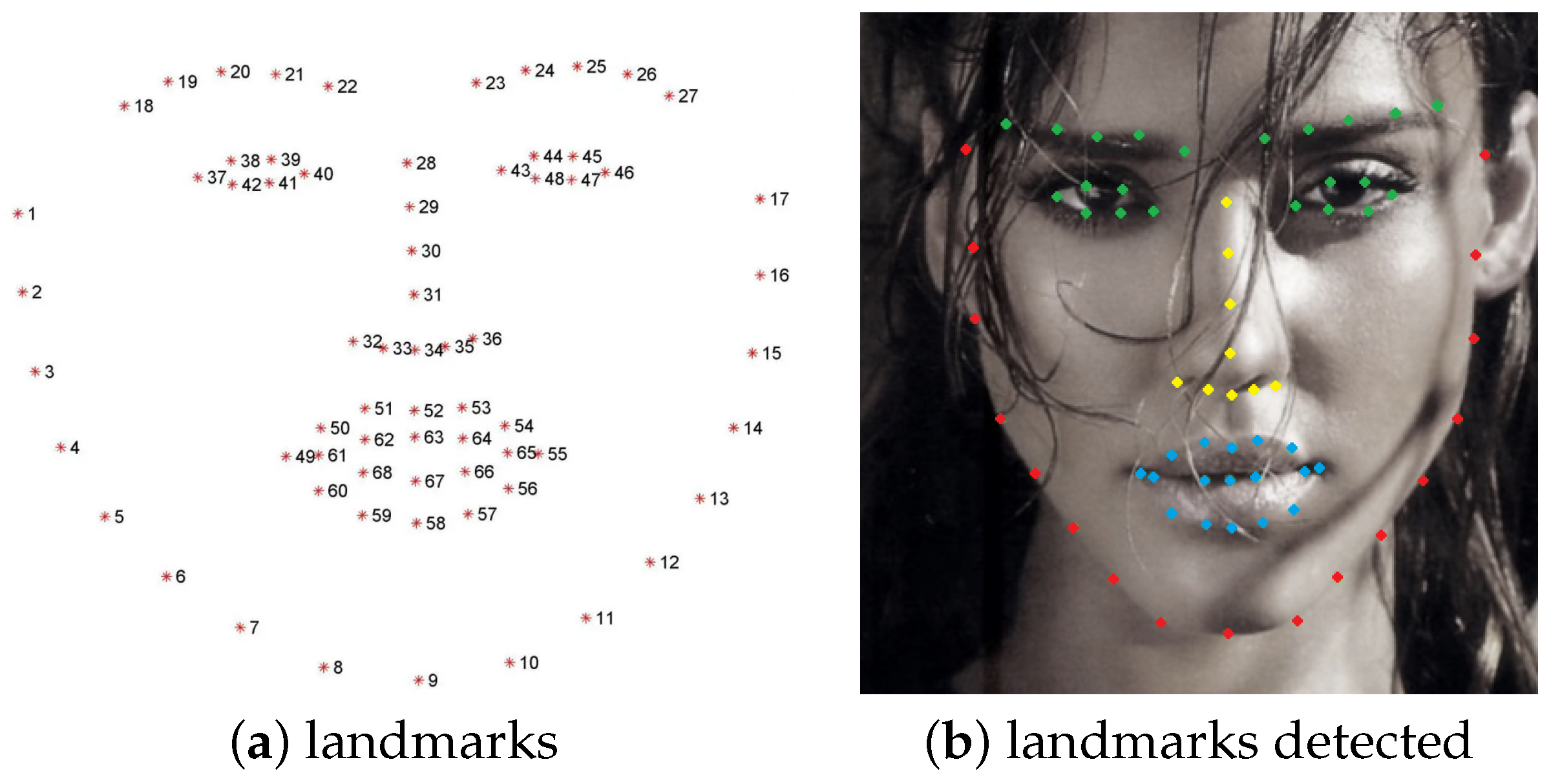
  • Facial landmarks: proposed in [28] and available in the https://github.com/davisking/dlib (accessed on 30 December 2022) library, the landmark localization algorithm returns 68 facial landmarks related to key facial structures. Those can be further partitioned into different face areas (face line, eyebrows, eyes, nose, and mouth), as is shown in Figure 5. This feature extractor outputs the arrays F I and F R of size 68 × 2 , containing row-wise, the 2D coordinates of the 68 landmarks, and we extract from them two types of differential feature vectors:
    LM 68 R 68 contains the Euclidean distances between F I [ i , : ] and F R [ i , : ] , i = 1 , 68 (i.e., the 2D coordinates of corresponding landmarks in the two different faces);
    LM 136 R 136 contains the differences in module between individual corresponding landmark coordinates F I [ i , j ] and F R [ i , j ] , i = 1 , 68 , j = 1 , 2 .

4. Experimental Setup and Analysis of Results

We report the results of our experimental campaign on synthetic and real face images of different sources, and by employing different metrics and feature representations for the joint analysis of x I and x R .
In particular, we considered the image data employed for the work [2], which have been made available by the authors (https://osf.io/ru36d/ (accessed on 30 December 2022)). They include synthetic images generated through StyleGAN2 (indicated as SG2), real images extracted from FFHQ (indicated as FFHQ), and the high-quality image dataset of human faces used for training StyleGAN2 (https://github.com/NVlabs/ffhq-dataset (accessed on 30 December 2022)).
Moreover, to diversify the data corpus and test generalization capabilities, we considered additional sets of real images coming from different sources, in particular:
Details about the data used in the experiments are reported in Figure 6.
For each image, we applied the inversion process and obtained its reconstructed version; we used the default parameters of the inversion algorithms and fixed the random seed for reproducibility. As a pre-processing step for all images before the inversion, we detected the squared area containing the face through the https://github.com/davisking/dlib (accessed on 30 December 2022) library, and blurred the background outside that area to retain mostly face information in the input data. If needed, we resized the area (using the https://pillow.readthedocs.io/en/stable/ (accessed on 30 December 2022) library) to the resolution 1024 × 1024, which is the one accepted by the inversion algorithm. The average time for reconstructing an input image on an NVIDIA RTX 3090 GPU is 90 s.
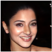
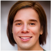
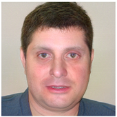
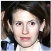
Examples of input and reconstructed images are reported in Table 1. We also release the input and reconstructed images https://tinyurl.com/puusfcke (accessed on 30 December 2022).
From visual inspection, it can be noticed that the face attributes of the synthetic image are reconstructed very accurately, while more pronounced discrepancies in the biometric traits are present for real images. In the following, we jointly study the image faces given as input to the inversion process and their reconstructed counterparts, thus, x I and x R .

4.1. Metrics-Based Analysis

First, we perform a similarity analysis between each image and its reconstructed counterpart. We considered the following metrics:
  • Mean Squared Error (MSE): Computes the distance pixel-wise between the two images
    M S E ( x I , x R ) = 1 M N n = 1 N m = 1 M k = 1 3 ( x I ( n , m , k ) x R ( n , m , k ) ) 2
    where M,N are the dimensions of the image (equal for both images); x I is the RGB input image and its x R reconstructed version.
  • Structure Similarity Index Method (SSIM): it is a perception-based model that takes into account the mean values and the variances of the two images
    S S I M ( x I , x R ) = ( 2 μ I μ R + c 1 ) ( 2 σ I R + c 2 ) ( μ I 2 + μ R 2 + c 1 ) ( σ I 2 + σ R 2 + c 2 )
    with μ I , μ R being the mean values of the two images, σ I , σ R variance of the two images, and c 1 and c 2 being stabilization factors.
  • Learned Perceptual Image Patch Similarity (LPIPS) (https://github.com/richzhang/PerceptualSimilarity (accessed on 30 December 2022)): it is proposed in [31] and used in [4] for the same purpose; it computes the similarity between the activations of two image patches for some pre-defined network. A low LPIPS score means that the image patches are perceptually similar.
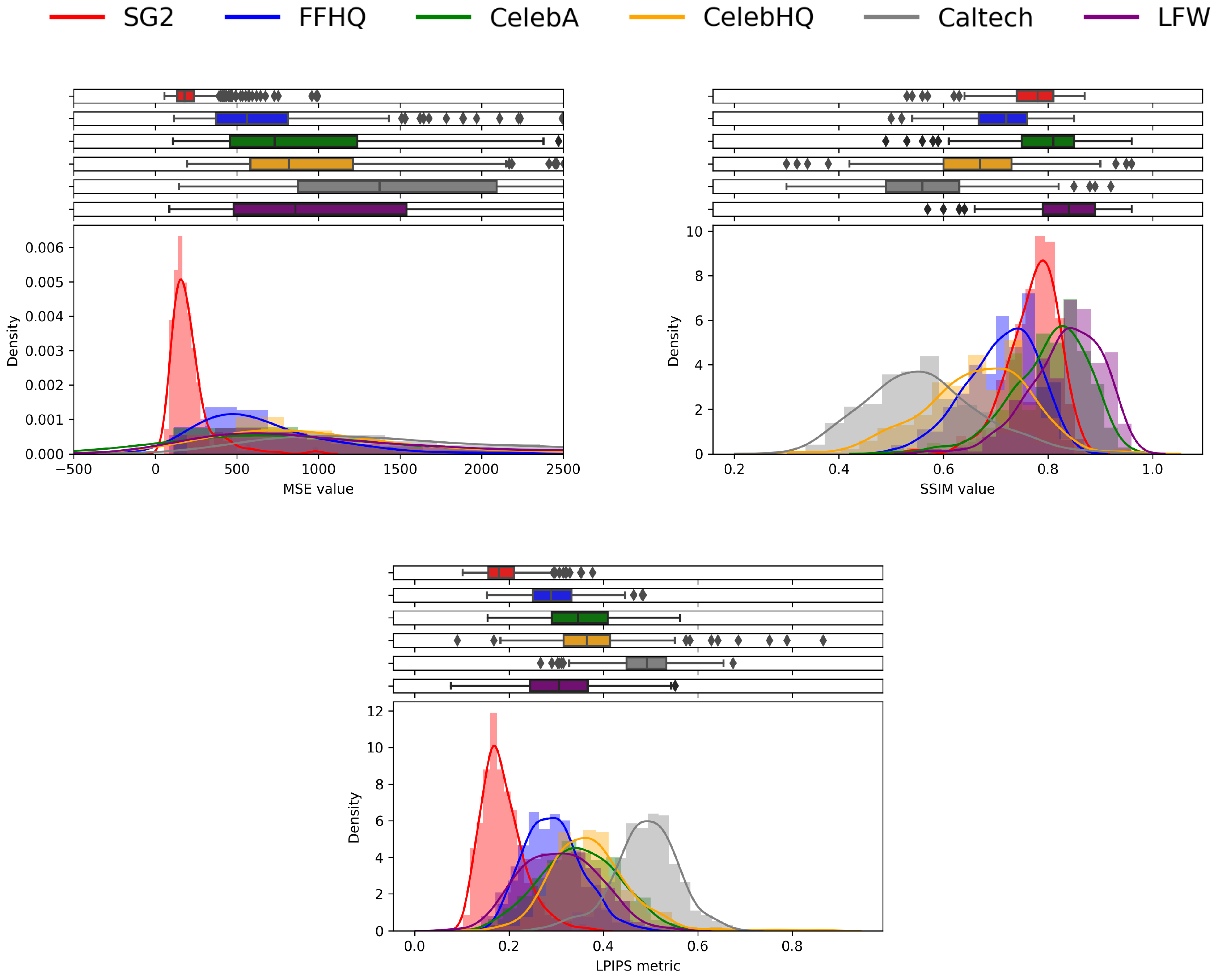
The results are reported in Figure 7. We can notice that SSIM histograms do not show a clear distinction among different clusters. Indeed, SSIM is sensitive to the perceivable changes in terms of structural information, which are usually not noticeable in GAN-generated images. On the contrary, we observe that pairs deriving from real images yield generally higher MSEs than the ones derived from synthetic faces (red histogram), making it evident that reconstructing a pointwise equal image of an unknown target is much more difficult. The same happens for the LPIPS metrics, where, following what was observed in [4], the SG2 images yield a higher similarity with their reconstructed counterparts.
Moreover, real images belonging to different datasets lead to different distributions, both in terms of LPIPS and MSE. In particular, it is interesting to observe that FFHQ images (blue histogram) present significantly lower values concerning other sources of real images: this may be related to the fact that those images were included in the training set of StyleGAN2, and thus, they are known to the generator.

4.2. Classification Results

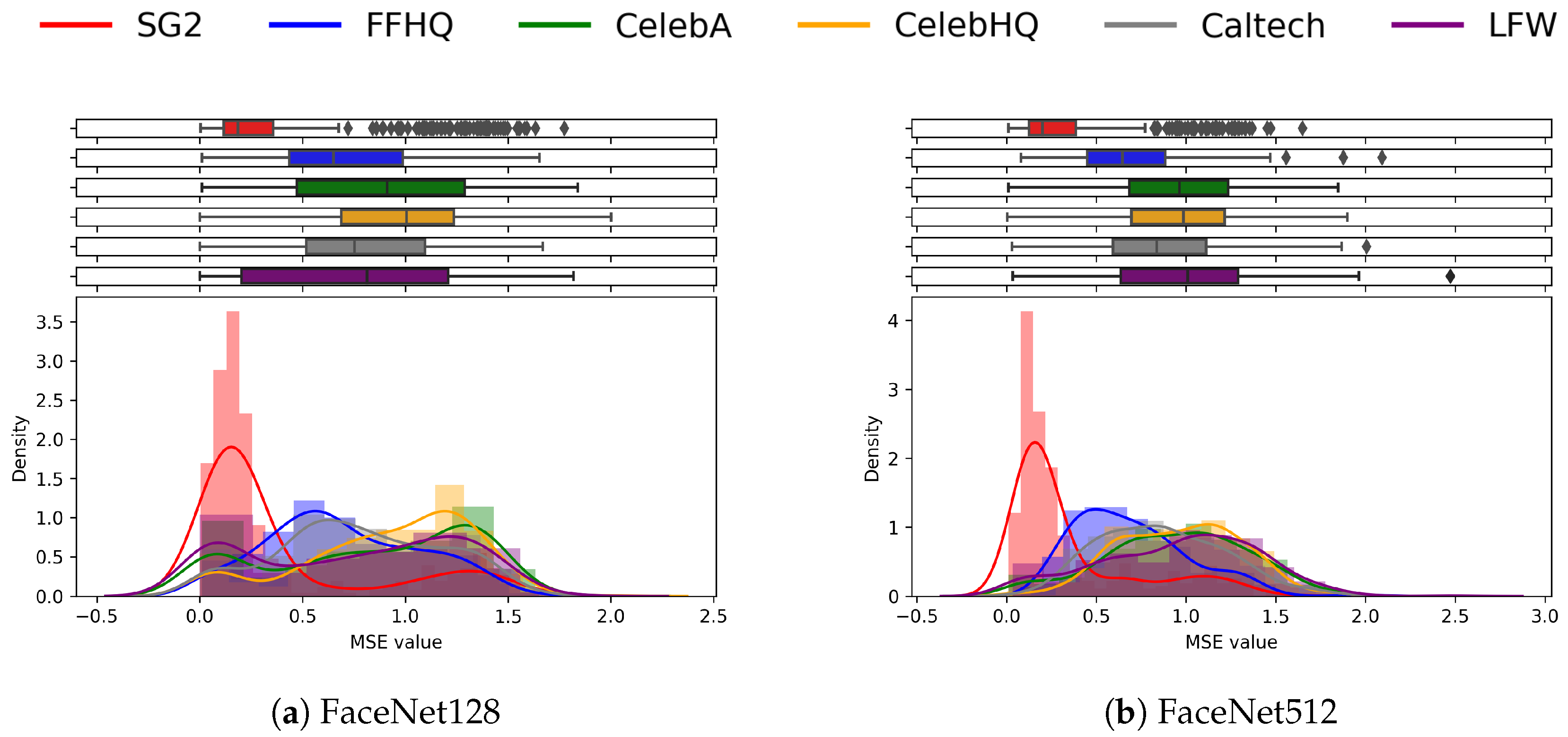
We now report the results of the classification analysis performed according to the pipeline proposed in Figure 4. First, we plot the histogram of the MSE between F I and F R among the different datasets. In Figure 8, we observe that both FaceNet embeddings are able to improve the discrimination capability already observed on Figure 7. In this representation, the images generated with SG2 produce a clear peak around low MSE values, with a rather limited overlap with the other clusters. As expected, the FFHQ image pairs lie between synthetic samples and other real ones.
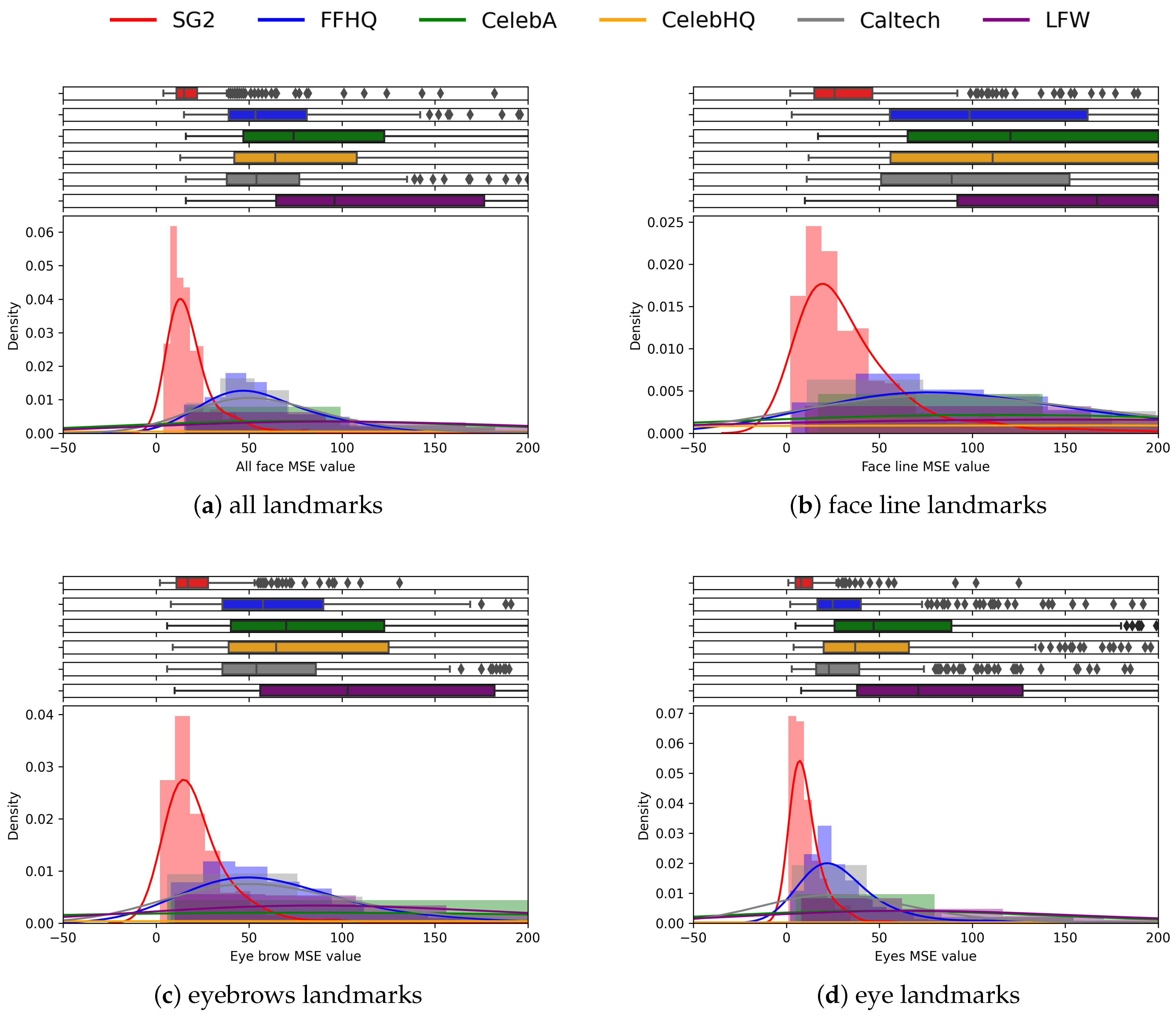
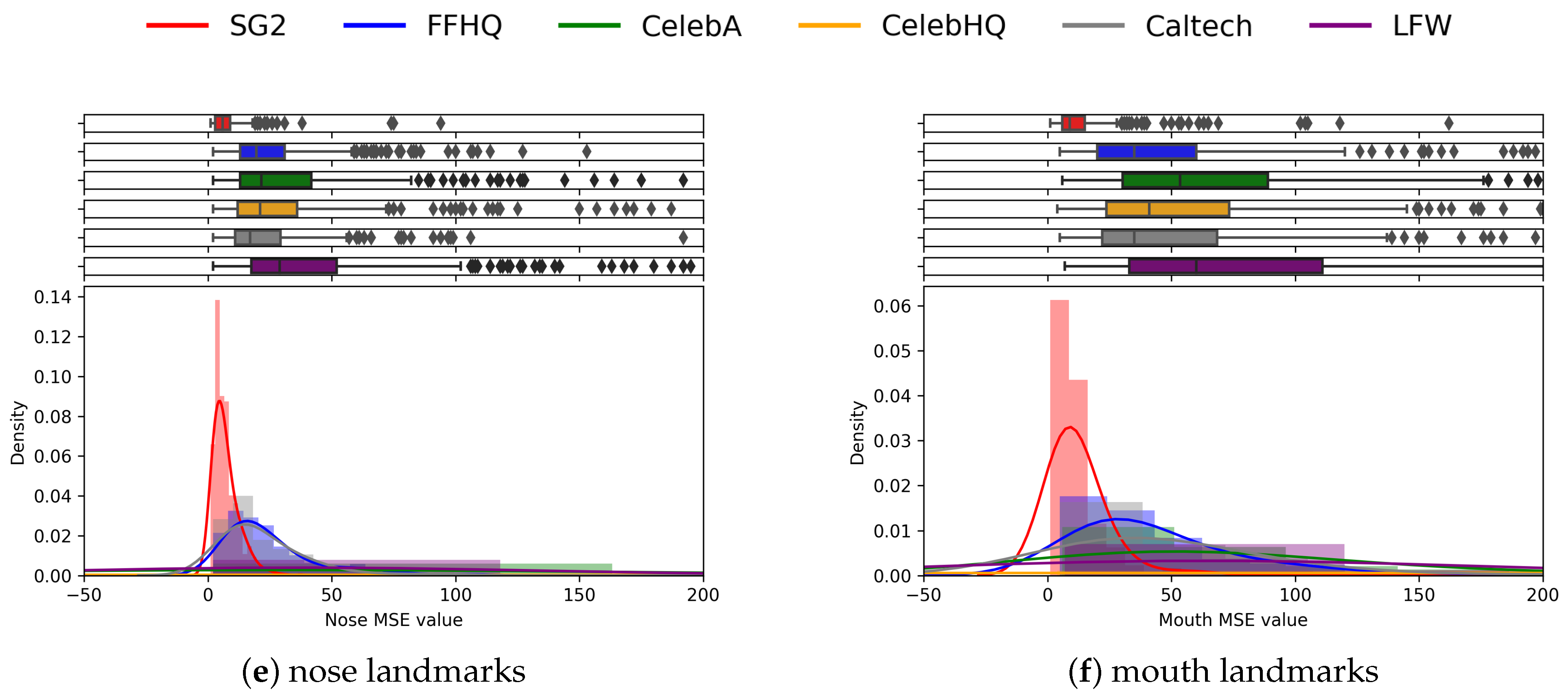
The charts reported in Figure 9 propose an analysis of the individual subsets of landmarks, according to the face area in which they belong (see Figure 5). These plots allow us to grasp the importance and the specific contribution of different sets of landmarks corresponding to different areas in the face. Indeed, the face line and eyes areas (eyes and eyebrows landmarks) clearly highlight the differences between real and synthetic pairs (see Figure 9b–d), while the nose and mouth areas are less effective in discrimination (Figure 9e–f). Anyway, the whole set of landmarks leads to the strongest separation, and is therefore used for further analysis.
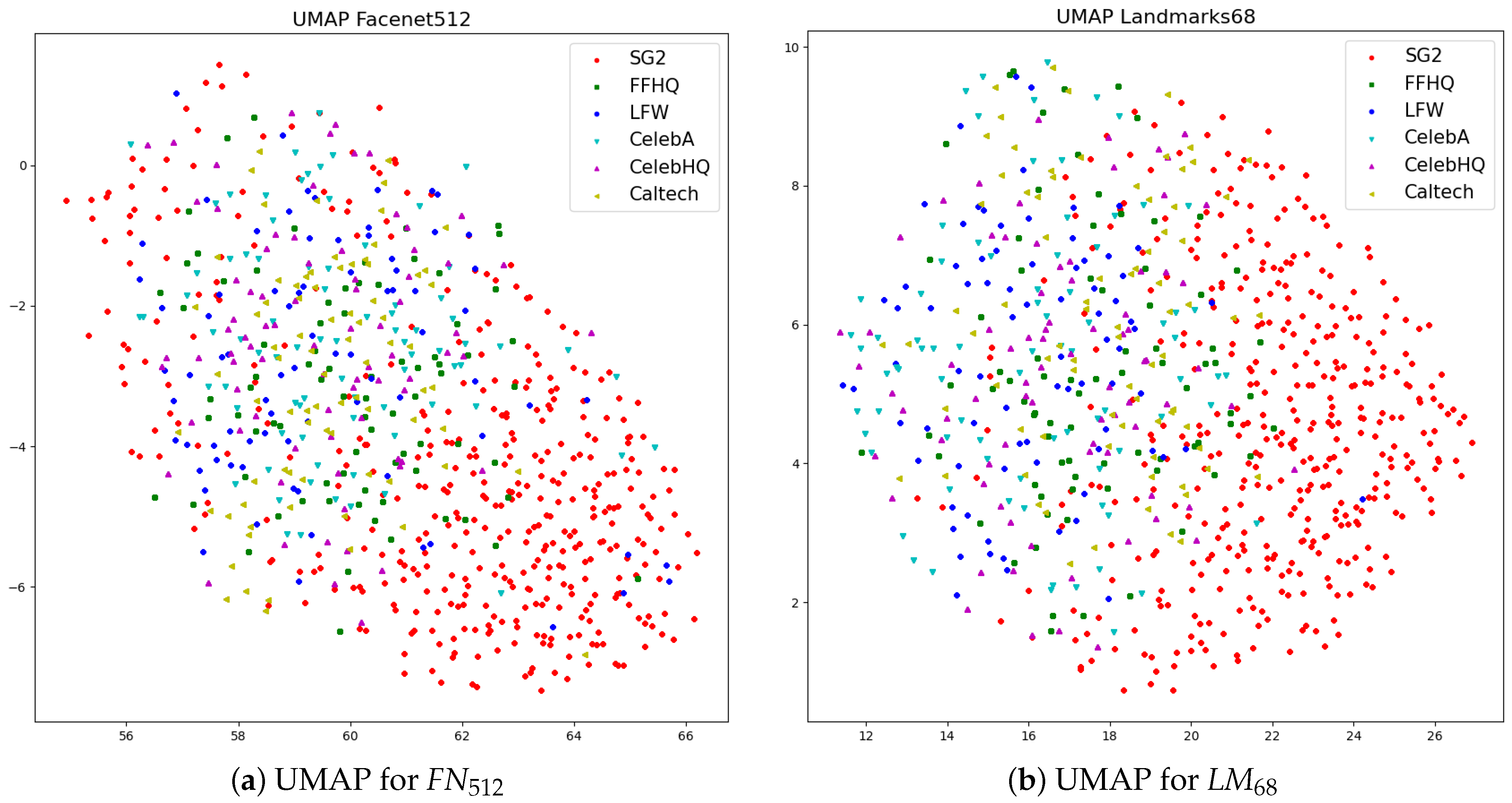
The UMAP visualization of the FN 512 and LM 68 differential features (Figure 10) provides a 2D view of the distribution of different pairs: while pairs deriving from real images of different sources essentially overlap, real and synthetic pairs clearly tend to cluster together.
For performing training and inference, we split our datasets into fixed train and test sets. In particular, we used 80 % of images from each dataset for training, and the remaining 20 % for testing. Different classifiers are used for comparative analysis; in particular, Support Vector Machines (SVMs), Random Forest (RF), Logistic Regression (LR), and Multilayer Perceptrons (MLPs), as provided in https://scikit-learn.org/stable/modules/generated/sklearn.svm.SVC.html (accessed on 30 December 2022) tool. We employed algorithms with default parameters and applied grid search for optimizing hyperparameters. In addition, we tested the Feedforward Neural Network (FNN) model provided by https://www.deeplearningwizard.com/deep_learning/practical_pytorch/pytorch_feedforward_neuralnetwork/ (accessed on 30 December 2022).
The results obtained with different types of differential vectors are reported in the following Table 2a–d. We first tested the datasets of real images individually against the SG2 data (indicated as * vs. SG2), as well as their union (indicated as All vs. SG2), yielding six different settings reported row-wise in the tables.
We observe that the SVM provides, on average, better results, and also in front of limited computational complexity. In addition, we verified that the Radial Basis Function (RBF) kernel with hyperparameter C = 1 consistently yields the best performance; thus, we select it as the reference model for the following experimental analyses. In terms of computational efficiency, the training time of SVM models is in the order of milliseconds, thus, it is negligible with respect to the inversion time.
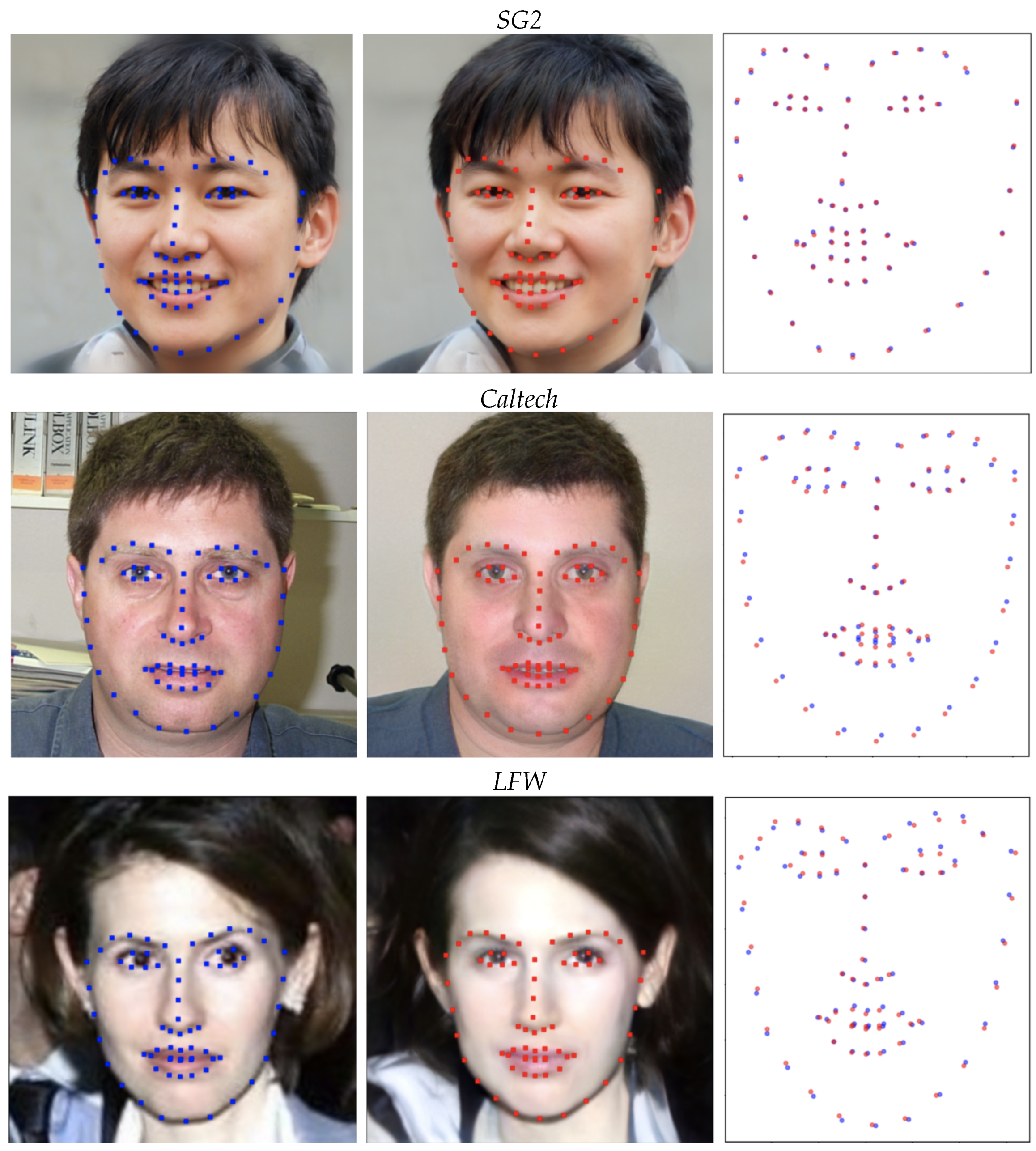
Interestingly, the landmark-based differential analysis yields substantially higher discrimination capabilities with respect to the FaceNet-based one, despite their generally lower dimensionality. In particular, they perform exceptionally well on the LFW pairs, which are the more critical case for the FaceNet representations. For a better understanding, we report in Figure 11 a comparative visualization of the landmarks detected in the input and reconstructed faces, and we plot them together to visualize the misalignment. It can be seen that the synthetic StyleGAN2 image pairs present almost overlapping landmarks, while the real ones show irregular displacements of individual landmarks.
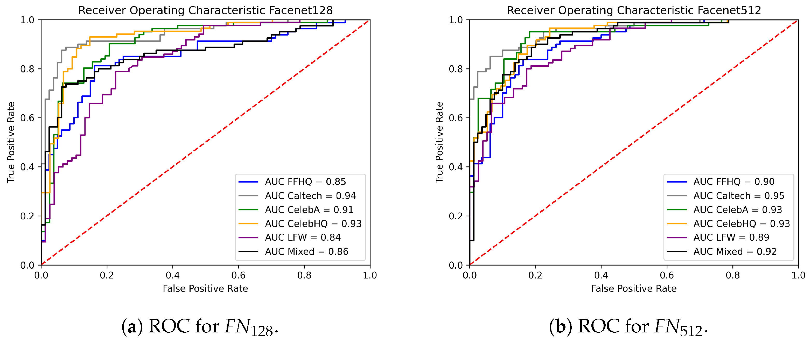
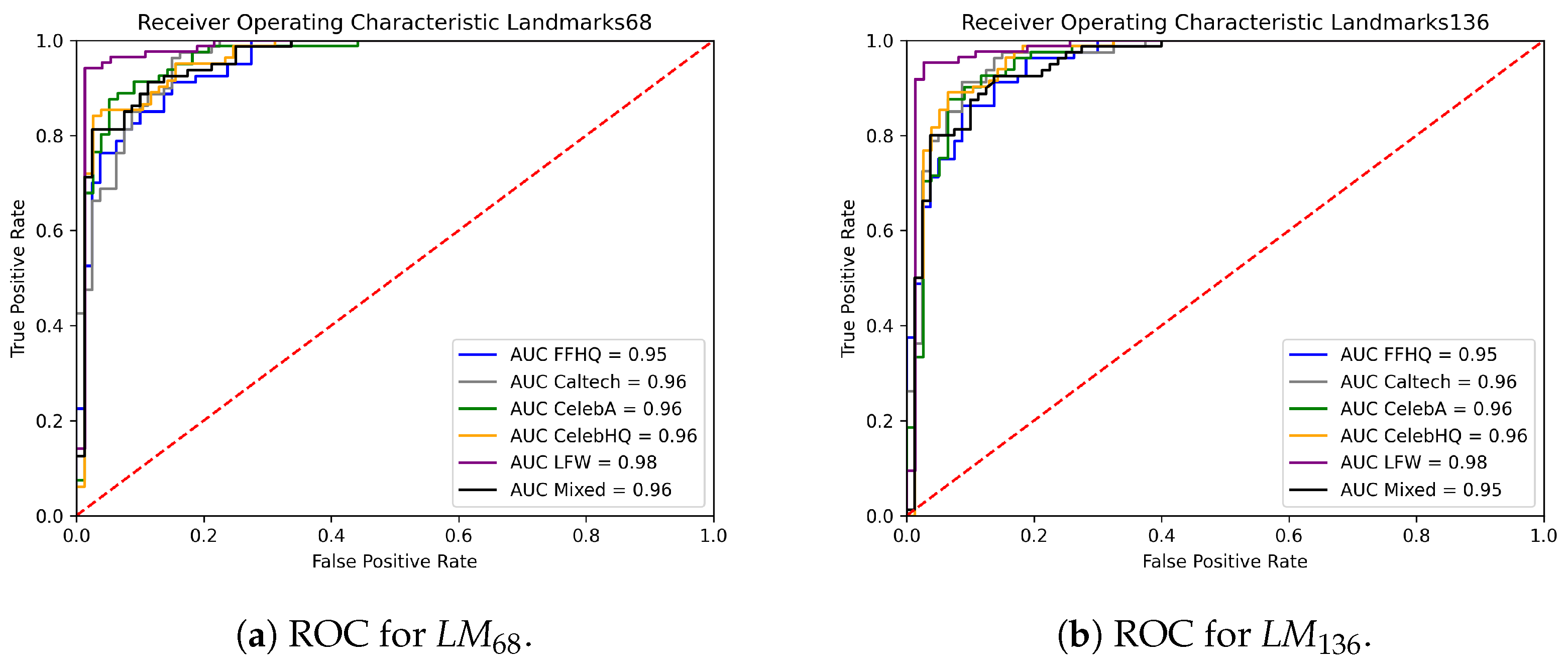
In general, the FFHQ pairs seem to be the harder ones to distinguish from SG2 pairs also for landmark-based features, possibly because the former were employed for training the StyleGAN2 generator. This is also observed in Figure 12 and Figure 13, where the ROC curves of the different classification scenarios and feature representations are reported. Even if the results are very good in all cases, Table 3 shows that AUC values for the LM 68 and LM 136 case remain lower for the FFHQ data with respect to other real images.

4.3. Robustness Analysis

An aspect of high practical relevance is whether synthetic images are still identified through the inversion-based analysis, even though they are not the direct output of the generator, but undergo successive post-processing. An advantage of facial landmarks is the fact that their detection and localization are rather robust to the operations applied to the images under analysis. FaceNet embeddings are also designed to generalize to different face image scales and conditions.
Since handling the variety of (even slight) potential operations is a known issue for data-driven techniques based on learned features, we now assess the robustness of the classifiers developed in Section 4.2 when training and testing data are not aligned in terms of post-processing. In this view, we study three routinely applied operations in the lifecycle of digital images, namely resizing, JPEG compression, and social network sharing. For the sake of conciseness, we focus on the case of FFHQ vs. SG2, which is the most critical one for the best-performing features.

4.3.1. Resizing

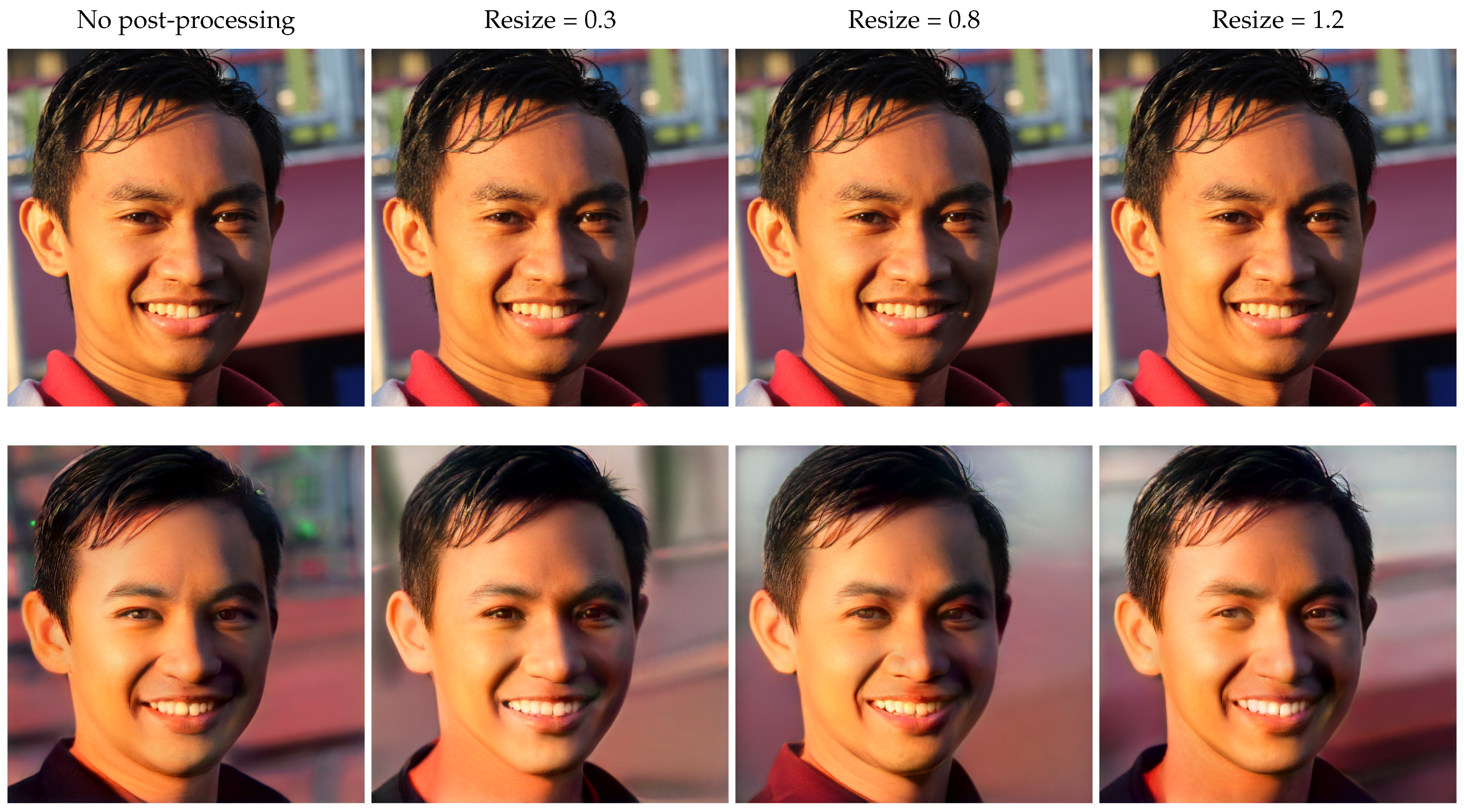
We have tested our discrimination models with inputs at different resolution levels by downscaling and upscaling the images. In particular, we rescale the entire datasets at different scaling factors { 0.3 , 0.7 , 0.8 , 0.9 , 1.1 , 1.2 , 1.3 } , we apply the inversion/reconstruction process for each case, and finally, we compute the differential feature vectors, FN 128 , FN 512 , LM 68 , and LM 136 . The library used for the resize process is https://pillow.readthedocs.io/en/stable/ (accessed on 30 December 2022), with the nearest neighbor resample parameter set (PIL.Image.NEAREST in the code). Since the StyleGAN2 inversion algorithm requires inputs with fixed size 1024 × 1024 pixels, when inverting images of different resolutions, a further cropping/rescaling operation is needed to meet this requirement. In doing so, some details of the image change in terms of quality (see Figure 14), making the discrimination between real images and fake images in principle harder.
After having scaled all the images, we trained and tested the models with these resized examples. Table 4, Table 5, Table 6 and Table 7 report the results obtained, where the training scaling factors are reported row-wise, and the testing scaling factors column-wise. Rows and columns with a scaling factor of 1.0 correspond to the baseline case (no scaling), where no post-processing is applied to either training or testing images. We notice that the accuracies are generally preserved and they present no dramatic drops, but rather, oscillations around the aligned cases corresponding to the diagonal values. For the majority of classifiers, the average variation over different testing sets does not exceed 2%.
Among the different representations, the FaceNet-based features seem to struggle more with the upscaled images rather than the downscaled ones, occasionally decreasing below 80%. This behavior is reversed for landmark-based features, for which the performances are more stable for upscaling factors and more sensible and oscillatory for downscaling ones. In both cases, the dimensionality of the differential vectors does not have a significant impact.

4.3.2. JPEG Compression

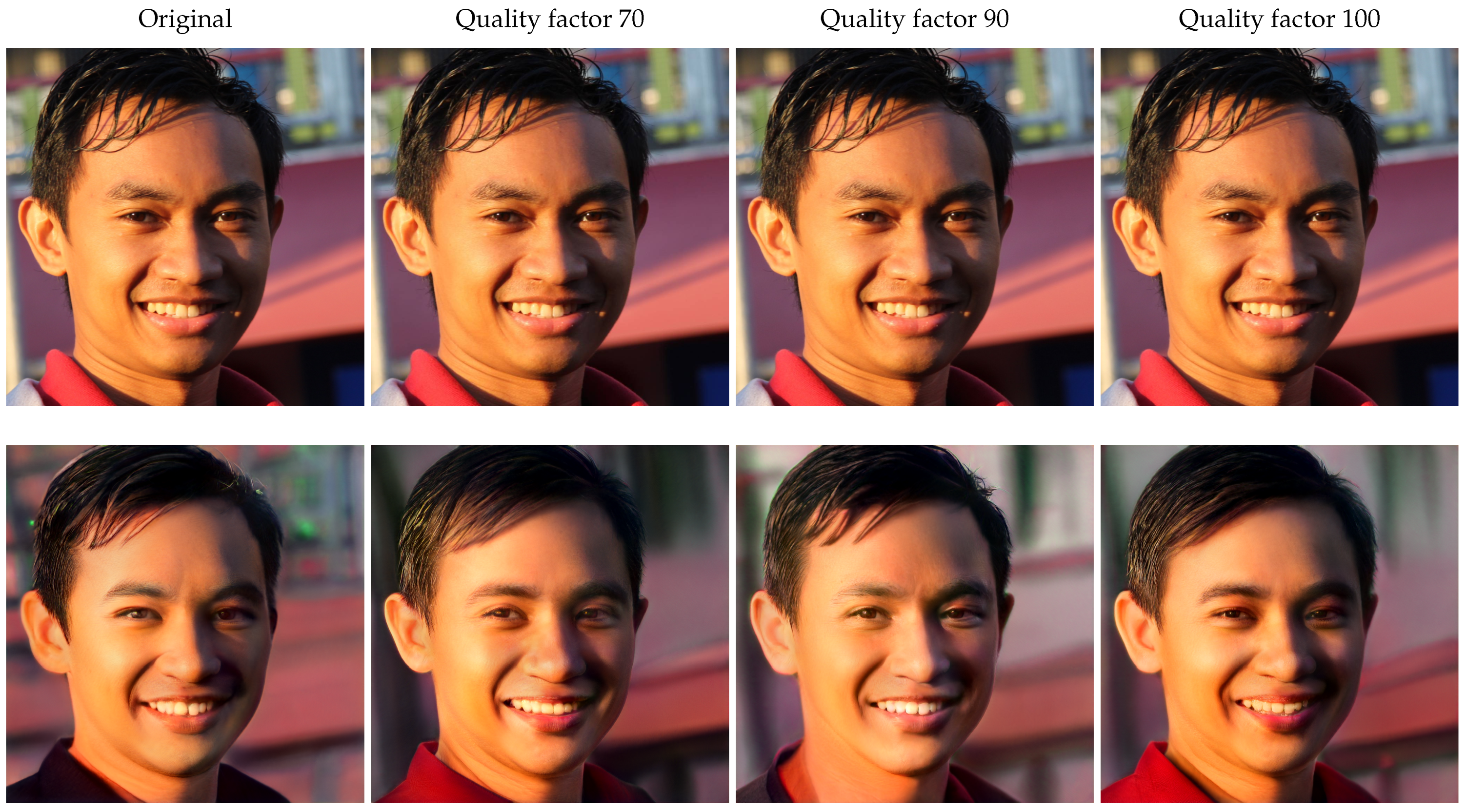
We apply the same robustness analysis for the JPEG compression at different quality factors { 100 , 95 , 90 , 80 , 70 } . Examples of compressed images and their reconstructions are reported in Figure 15.
The results are reported in Table 8, Table 9, Table 10 and Table 11. As for the resizing section, the library used for the compression process is https://pillow.readthedocs.io/en/stable/ (accessed on 30 December 2022). We varied the quality parameter of the saved image. The baseline case is reported in the ’NO COMP’ rows and columns. Additionally, in this case, all of the feature representations generally retain their accuracies when the training and testing sets are misaligned, as most of the models have an average deviation from the aligned case below 2%.
Interestingly, when observing the results column-wise, we notice that for FaceNet-based features, a stronger JPEG compression consistently degrades the average performance of the classifiers; as opposed to that, LM 68 and LM 136 fully retain their accuracy, thus strengthening the observation that such semantic cues yield an improved robustness to post-processing.

4.3.3. Social Network Sharing

The identification of synthetic media over social networks is a well-known challenge in media forensics [32], and an open issue for GAN-generated image detection [33]. Social media typically apply custom data compression algorithms to reduce the size and the quality of the images to be stored on data centers or costumer’s devices, thus hindering post hoc analyses.
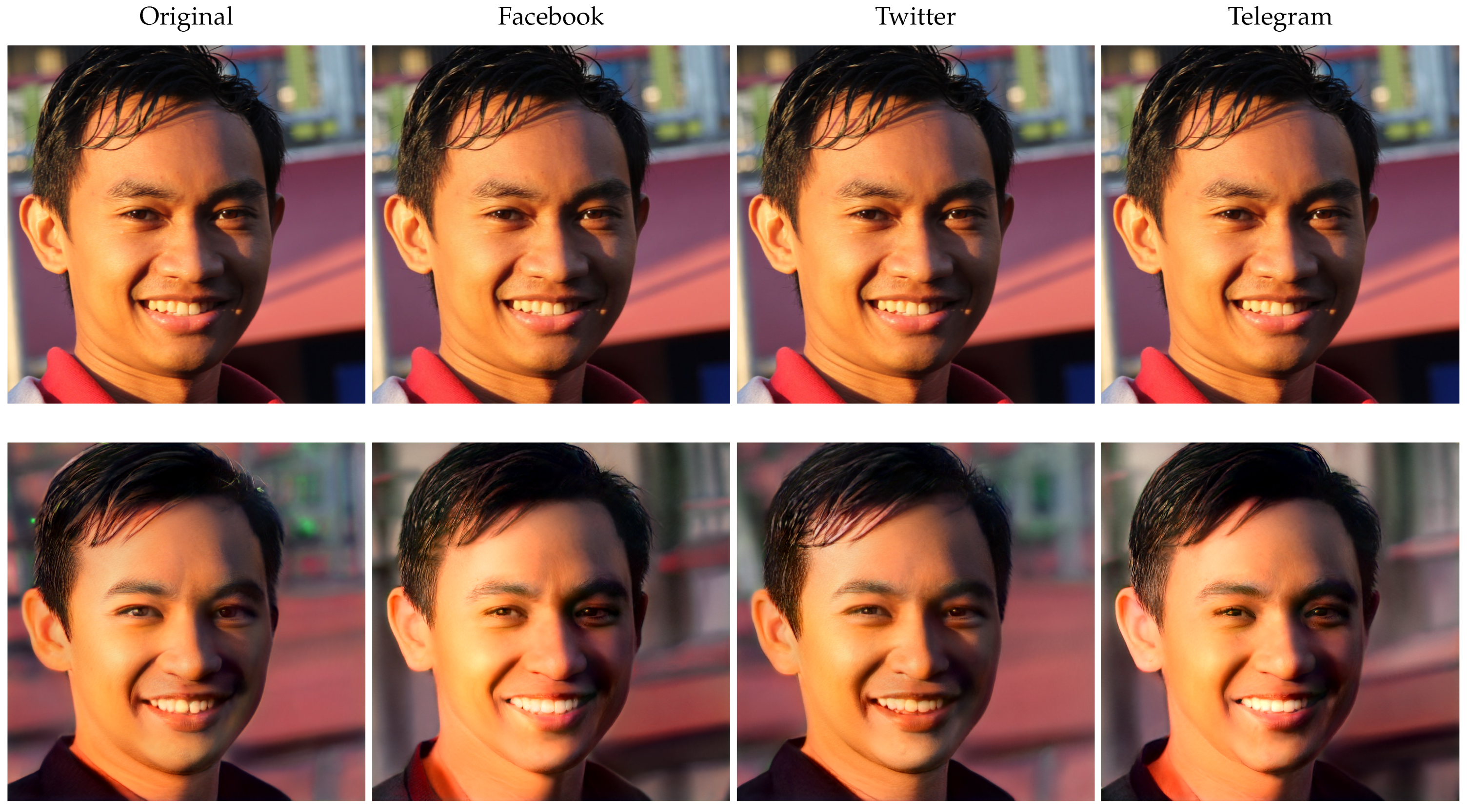
We then test the capabilities of the developed classifiers to generalize to the image data shared on social networks. It is worth noticing that in this case, the models are exactly the ones considered in the classifiers developed in Section 4.2; thus, they are trained entirely on images with no sharing operations. Instead, the testing set is a subset of the recently published https://zenodo.org/record/7065064#.Y2to3ZzMKdZ (accessed on 30 December 2022) dataset, which is composed of StyleGAN2 images and real images (extracted from FFHQ) before and after the upload and download from three different social networks: Facebook, Telegram, and Twitter. We randomly select 100 synthetic and 100 real images and extract their shared versions through the three platforms.
Examples of shared images and their reconstructions are reported in Figure 16.
After inversion, we obtain a reconstruction for each of them. If needed, a rescaling operation is applied to fit the input size of the inversion algorithm. We then extract the feature representations and differential vectors, and test them through the corresponding classifiers already trained in Section 4.2 for the FFHQ vs. SG2 scenario.
The results are reported in Table 12, where the accuracies of each binary classification scenario (one for each platform) are reported column-wise. As highlighted in [33], all platforms apply JPEG compression (quality factor between 80 and 90), and Facebook also resizes the images by a 0.7 factor.
Interestingly, the landmark-based features yield remarkable performance in all cases, thus demonstrating a high robustness against this realistic kind of post-processing. In particular, they achieve a maximum accuracy in the Facebook case, which is the more critical one for FaceNet-based features, and also for the general purpose deep networks analyzed in [33].

5. Conclusions

We have explored a forensic detection strategy for identifying synthetic face images based on the inversion of the GAN synthesis process. The experimental results demonstrate that a proper biometric comparison between the image under investigation and its reconstruction through an inversion algorithm allows for distinguishing images that have been synthesized by the considered generator and those who are not. In particular, our analysis shows that landmark-based feature representations are particularly effective for this purpose.
A desirable aspect of such an approach is that it is not purely inductive, but is based on the very architecture of the generation methods. Moreover, the best-performing features refer to an explicit face model, and they express a biometric reconstruction dissimilarity that can be better interpreted with respect to deep representations.
On the other hand, a limitation of this approach is that it assumes prior knowledge of the candidate generator, for which an inversion procedure needs to be devised. In particular, this work focuses on a powerful yet single generator. Extensions of this work would consider more general scenarios where the inversion-based comparison is tested against multiple latest generators, such as StyleGAN3 [34] and EG3D [35]. This would also include dealing with more comprehensive data corpora with diverse facial attributes in terms of expression, gender or age, as well as more generative models that are trained to synthesize other objects beyond faces. Moreover, an effective fusion of our approach with data-driven techniques would be a promising direction for future investigations. In addition, an open research question is to which extent inversion-based techniques can be applied to generative models operating in domains other then the visual one, such as speech [36], text [37], or raw tabular data [38]. In this respect, we expect that the main concept of the paper still remains valid, while the metrics should be suitably revised to capture the most significant domain-sensitive differences.

Author Contributions

Conceptualization, C.P.; Data curation, F.L., D.L., and G.A.; Methodology, C.P., F.L., D.L., G.A., G.B., and F.D.N.; Project administration, C.P.; Software, F.L., D.L., and G.A.; Supervision, C.P., G.B., and F.D.N.; Writing—original draft, C.P., F.L., D.L., and G.A.; Writing—review and editing, G.B. and F.D.N. All authors have read and agreed to the published version of the manuscript.

Funding

This work has received funding by the project PREMIER (PREserving Media trustworthiness in the artificial Intelligence ERa) under contract PRIN 2017 2017Z595XS-001, funded by the Italian Ministry of University and Research, from the TruBlo consortium as part of the TrueBees project (https://www.trublo.eu/truebees/ (accessed on 30 December 2022)) funded by TruBlo under the Europe’s Horizon 2020 programme (grant agreement No. 957228), and by the Defense Advanced Research Projects Agency (DARPA) under Agreement No. HR00112090136.

Institutional Review Board Statement

Not applicable.

Informed Consent Statement

Not applicable.

Data Availability Statement

The dataset of reconstructed images is available at https://tinyurl.com/puusfcke (accessed on 30 December 2022).

Conflicts of Interest

The authors declare no conflict of interest.

References

  1. Lago, F.; Pasquini, C.; Böhme, R.; Dumont, H.; Goffaux, V.; Boato, G. More Real Than Real: A Study on Human Visual Perception of Synthetic Faces. IEEE Signal Process. Mag. 2021, 39, 109–116. [Google Scholar] [CrossRef]
  2. Nightingale, S.J.; Farid, H. AI-synthesized faces are indistinguishable from real faces and more trustworthy. Proc. Natl. Acad. Sci. USA 2022, 119, e2120481119. [Google Scholar] [CrossRef] [PubMed]
  3. Karras, T.; Laine, S.; Aila, T. A style-based generator architecture for generative adversarial networks. In Proceedings of the IEEE/CVF Conference on Computer Vision and Pattern Recognition (CVPR), Long Beach, CA, USA, 15–20 June 2019; pp. 4401–4410. [Google Scholar]
  4. Karras, T.; Laine, S.; Aittala, M.; Hellsten, J.; Lehtinen, J.; Aila, T. Analyzing and Improving the Image Quality of StyleGAN. In Proceedings of the IEEE/CVF Conference on Computer Vision and Pattern Recognition (CVPR), Seattle, WA, USA, 13–19 June 2020. [Google Scholar]
  5. Dang-Nguyen, D.T.; Boato, G.; De Natale, F.G. 3D-model-based video analysis for computer generated faces identification. IEEE Trans. Inf. Forensics Secur. 2015, 10, 1752–1763. [Google Scholar] [CrossRef]
  6. Bonomi, M.; Pasquini, C.; Boato, G. Dynamic texture analysis for detecting fake faces in video sequences. J. Vis. Commun. Image Represent. 2021, 79, 103239. [Google Scholar] [CrossRef]
  7. Dang-Nguyen, D.; Boato, G.; De Natale, F. Identify computer generated characters by analysing facial expressions variation. In Proceedings of the IEEE International Workshop on Information Forensics and Security, Tenerife, Spain, 2–5 December 2012; pp. 252–257. [Google Scholar]
  8. Gragnaniello, D.; Cozzolino, D.; Marra, F.; Poggi, G.; Verdoliva, L. Are GAN generated images easy to detect? A critical analysis of the state-of-the-art. In Proceedings of the IEEE International Conference on Multimedia and Expo, Shenzhen, China, 5–9 July 2021; pp. 1–6. [Google Scholar]
  9. Marra, F.; Saltori, C.; Boato, G.; Verdoliva, L. Incremental learning for the detection and classification of GAN-generated images. In Proceedings of the IEEE International Workshop on Information Forensics and Security, Delft, The Netherlands, 9–12 December 2019; pp. 1–6. [Google Scholar]
  10. Marra, F.; Gragnaniello, D.; Verdoliva, L.; Poggi, G. Do GANs leave artificial fingerprints? In Proceedings of the IEEE Conference on Multimedia Information Processing and Retrieval, San Jose, CA, USA, 28–30 March 2019; pp. 506–511. [Google Scholar]
  11. Wang, S.Y.; Wang, O.; Zhang, R.; Owens, A.; Efros, A.A. CNN-generated images are surprisingly easy to spot... for now. In Proceedings of the IEEE/CVF Conference on Computer Vision and Pattern Recognition (CVPR), Seattle, WA, USA, 13–19 June 2020; pp. 8695–8704. [Google Scholar]
  12. Xia, W.; Zhang, Y.; Yang, Y.; Xue, J.H.; Zhou, B.; Yang, M.H. GAN Inversion: A Survey. IEEE Trans. Pattern Anal. Mach. Intell. 2022, 1–17. [Google Scholar] [CrossRef]
  13. Nataraj, L.; Mohammed, T.M.; Manjunath, B.S.; Chandrasekaran, S.; FlennerJawadul, A.; Bappy, H.; Roy-Chowdhury, A.K. Detecting GAN generated Fake Images using Co-occurrence Matrices. Electron. Imaging 2019, 2019, 532-1. [Google Scholar] [CrossRef] [Green Version]
  14. Wang, R.; Juefei-Xu, F.; Ma, L.; Xie, X.; Huang, Y.; Wang, J.; Liu, Y. FakeSpotter: A Simple yet Robust Baseline for Spotting AI-Synthesized Fake Faces. In Proceedings of the International Joint Conference on Artificial Intelligence (IJCAI), Yokohama, Japan, 7–15 January 2020. [Google Scholar]
  15. Marcon, F.; Pasquini, C.; Boato, G. Detection of Manipulated Face Videos over Social Networks: A Large-Scale Study. J. Imaging 2021, 7, 193. [Google Scholar] [CrossRef] [PubMed]
  16. Dong, X.; Miao, Z.; Ma, L.; Shen, J.; Jin, Z.; Guo, Z.; Teoh, A.B.J. Reconstruct face from features based on genetic algorithm using GAN generator as a distribution constraint. Comput. Secur. 2023, 125, 103026. [Google Scholar] [CrossRef]
  17. Albright, M.; McCloskey, S. Source Generator Attribution via Inversion. In Proceedings of the IEEE/CVF Conference on Computer Vision and Pattern Recognition (CVPR) Workshops, Long Beach, CA, USA, 16–20 June 2019. [Google Scholar]
  18. Scherhag, U.; Rathgeb, C.; Merkle, J.; Busch, C. Deep Face Representations for Differential Morphing Attack Detection. IEEE Trans. Inf. Forensics Secur. 2020, 15, 3625–3639. [Google Scholar] [CrossRef]
  19. Autherith, S.; Pasquini, C. Detecting morphing attacks through face geometry. J. Imaging 2020, 6, 115. [Google Scholar] [CrossRef] [PubMed]
  20. Chen, B.; Tang, G.; Sun, L.; Mao, X.; Guo, S.; Zhang, H.; Wang, X. Detection of GAN-Synthesized Image Based on Discrete Wavelet Transform. Secur. Commun. Netw. 2021, 2021, 5511435. [Google Scholar]
  21. Wang, J.; Tondi, B.; Barni, M. An Eyes-Based Siamese Neural Network for the Detection of GAN-Generated Face Images. Front. Signal Process. 2022, 45. [Google Scholar] [CrossRef]
  22. Agarwal, S.; Farid, H. Detecting deep-fake videos from aural and oral dynamics. In Proceedings of the IEEE/CVF conference on computer vision and pattern recognition (CVPR), Nashville, TN, USA, 20–25 June 2021; pp. 981–989. [Google Scholar]
  23. Schwarcz, S.; Chellappa, R. Finding facial forgery artifacts with parts-based detectors. In Proceedings of the IEEE/CVF Conference on Computer Vision and Pattern Recognition (CVPR), Nashville, TN, USA, 20–25 June 2021; pp. 933–942. [Google Scholar]
  24. Ju, Y.; Jia, S.; Ke, L.; Xue, H.; Nagano, K.; Lyu, S. Fusing Global and Local Features for Generalized AI-Synthesized Image Detection. arXiv 2022, arXiv:2203.13964R. [Google Scholar]
  25. Goodfellow, I.; Pouget-Abadie, J.; Mirza, M.; Xu, B.; Warde-Farley, D.; Ozair, S.; Courville, A.; Bengio, Y. Generative Adversarial Nets. In Proceedings of the Advances in Neural Information Processing Systems; Ghahramani; Ghahramani, Z., Welling, M., Cortes, C., Lawrence, N., Weinberger, K., Eds.; Curran Associates, Inc.: Red Hook, NY, USA, 2014; Volume 27. [Google Scholar]
  26. Schroff, F.; Kalenichenko, D.; Philbin, J. FaceNet: A unified embedding for face recognition and clustering. In Proceedings of the IEEE/CVF Conference on Computer Vision and Pattern Recognition (CVPR), Boston, MA, USA, 7–12 June 2015; pp. 815–823. [Google Scholar]
  27. Huang, G.B.; Ramesh, M.; Berg, T.; Learned-Miller, E. Labeled Faces in the Wild: A Database for Studying Face Recognition in Unconstrained Environments; Technical Report 07-49; University of Massachusetts: Amherst, MA, USA, 2007. [Google Scholar]
  28. Kazemi, V.; Sullivan, J. One millisecond face alignment with an ensemble of regression trees. In Proceedings of the IEEE/CFV Conference on Computer Vision and Pattern Recognition (CVPR), Columbus, OH, USA, 23–28 June 2014; pp. 1867–1874. [Google Scholar]
  29. Liu, Z.; Luo, P.; Wang, X.; Tang, X. Deep Learning Face Attributes in the Wild. In Proceedings of the International Conference on Computer Vision (ICCV), Santiago, Chile, 7–13 December 2015. [Google Scholar]
  30. Lee, C.H.; Liu, Z.; Wu, L.; Luo, P. MaskGAN: Towards Diverse and Interactive Facial Image Manipulation. In Proceedings of the IEEE/CVF Conference on Computer Vision and Pattern Recognition (CVPR), Seattle, WA, USA, 13–19 June 2020. [Google Scholar]
  31. Zhang, R.; Isola, P.; Efros, A.A.; Shechtman, E.; Wang, O. The Unreasonable Effectiveness of Deep Features as a Perceptual Metric. In Proceedings of the IEEE/CVF Conference on Computer Vision and Pattern Recognition (CVPR), Salt Lake City, UT, USA, 18–23 June 2018. [Google Scholar]
  32. Pasquini, C.; Amerini, I.; Boato, G. Media forensics on social media platforms: A survey. EURASIP J. Inf. Secur. 2021, 2021, 1–19. [Google Scholar] [CrossRef]
  33. Boato, G.; Pasquini, C.; Stefani, A.; Verde, S.; Miorandi, D. TrueFace: A dataset for the detection of synthetic face images from social networks. In Proceedings of the IEEE/IAPR International Joint Conference on Biometrics, Abu Dhabi, United Arab Emirates, 10–13 October 2022. [Google Scholar]
  34. Karras, T.; Aittala, M.; Laine, S.; Härkönen, E.; Hellsten, J.; Lehtinen, J.; Aila, T. Alias-Free Generative Adversarial Networks. In Proceedings of the NeurIPS, Virtual, 13 December 2021. [Google Scholar]
  35. Chan, E.R.; Lin, C.Z.; Chan, M.A.; Nagano, K.; Pan, B.; Mello, S.D.; Gallo, O.; Guibas, L.; Tremblay, J.; Khamis, S.; et al. Efficient Geometry-aware 3D Generative Adversarial Networks. In Proceedings of the IEEE/CVF Conference on Computer Vision and Pattern Recognition (CVPR), New Orleans, LA, USA, 19–20 June 2022. [Google Scholar]
  36. Bińkowski, M.; Donahue, J.; Dieleman, S.; Clark, A.; Elsen, E.; Casagrande, N.; Cobo, L.C. High Fidelity Speech Synthesis with Adversarial Networks. In Proceedings of the ICLR, Addis Ababa, Ethiopia, 26–30 April 2020. [Google Scholar]
  37. Xu, J.; Sun, X.; Ren, X.; Lin, J.; Wei, B.; Li, W. DP-GAN: Diversity-Promoting Generative Adversarial Network for Generating Informative and Diversified Text. arXiv 2018, arXiv:1802.01345. [Google Scholar]
  38. Bhavsar, K.; Vakharia, V.; Chaudhari, R.; Vora, J.; Pimenov, D.Y.; Giasin, K. A Comparative Study to Predict Bearing Degradation Using Discrete Wavelet Transform (DWT), Tabular Generative Adversarial Networks (TGAN) and Machine Learning Models. Machines 2022, 10, 176. [Google Scholar] [CrossRef]
Figure 1. Overview of the inversion-based detection.
Applsci 13 00816 g001
Figure 2. GAN architecture and training scheme.
Applsci 13 00816 g002
Figure 3. Examples of face images before (top row) and after (bottom row) the reconstruction using the inversion StyleGAN2 process available https://github.com/NVlabs/stylegan2-ada-pytorch/blob/main/projector.py (accessed on 30 December 2022).
Applsci 13 00816 g003
Figure 4. Pipeline of the comparison and training/classification processes.
Applsci 13 00816 g004
Figure 5. (a) Landmarks numbered from 1 to 68; (b) Landmarks detected on a face. We can identify 5 areas: face line (red landmarks [1–17]), eyebrows [18–27], and eyes [37–48], both in green (we call them eye area), nose [28–36] in yellow, and mouth [49–68] in blue.
Applsci 13 00816 g005
Figure 6. Summary of the face image data used in the experiments.
Applsci 13 00816 g006
Figure 7. Histograms of different similarity metrics for images belonging to different datasets and their reconstructed counterparts. For each case, we report the density of the values of each similarity metric and their https://seaborn.pydata.org/generated/seaborn.boxplot.html (accessed on 30 December 2022) on top of the histogram, highlighting the interval between the first and third quartiles of each dataset (colored box), the median value of the distribution (vertical line within the colored box), and the outliers (grey diamonds).
Applsci 13 00816 g007
Figure 8. Comparison between FaceNet128 and FaceNet512 features using the MSE. FaceNet512 shows better results: the SG2 faces are well separated with respect to the other datasets, where the distributions tend to overlap each other. FaceNet128 shows an overlap between SG2 and LFW.
Applsci 13 00816 g008
Figure 9. Plots above visualize the histograms of the distributions of the landmarks of different areas of the face for the different datasets. The full set of landmarks shows better discrimination capability.
Applsci 13 00816 g009aApplsci 13 00816 g009b
Figure 10. Visualization of FN 512 and LM 68 differential feature vectors through the UMAP dimensionality reduction.
Applsci 13 00816 g010
Figure 11. Visualization of the landmarks detected on the input and the reconstructed images from different datasets. In each case, the left image is the input one with the detected landmarks marked in blue, and the central one is the corresponding reconstruction with the detected landmarks marked in red. On the right, the two sets of landmarks are reported on the same spatial grid, so that their displacement can be visualized.
Applsci 13 00816 g011
Figure 12. Comparison of the ROC curves obtained with the SVM model using Facenet features.
Applsci 13 00816 g012
Figure 13. Comparison of the ROC curves obtained with the SVM model using landmark-based features.
Applsci 13 00816 g013
Figure 14. Examples of face images before (top row) and after (bottom row) the reconstruction when different resizing factors are applied as post-processing.
Applsci 13 00816 g014
Figure 15. Examples of face images before (top row) and after (bottom row) the reconstruction when different JPEG quality factors are applied as post-processing.
Applsci 13 00816 g015
Figure 16. Shared images before (top row) and after (bottom row) the reconstruction.
Applsci 13 00816 g016
Table 1. Examples of input face images and their reconstructions.
Dataset x I x R
SG2Applsci 13 00816 i001Applsci 13 00816 i002
FFHQApplsci 13 00816 i003Applsci 13 00816 i004
CelebAApplsci 13 00816 i005Applsci 13 00816 i006
CelebHQApplsci 13 00816 i007Applsci 13 00816 i008
CaltechApplsci 13 00816 i009Applsci 13 00816 i010
LFWApplsci 13 00816 i011Applsci 13 00816 i012
Table 2. Accuracy obtained with different data and classifiers (reported in percentage).
SVMRFLRMLPFNN
FFHQ vs. SG280.6376.8870.6370.6379.38
CelebA vs. SG282.2882.9169.6269.6282.91
CelebHQ vs. SG288.0586.1677.9977.9986.79
LFW vs. SG276.8874.3871.2573.1375.63
Caltech vs. SG289.3881.8881.2581.2583.13
All vs. SG278.1375.0071.8873.1377.50
(a) FN 128
SVMRFLRMLPFNN
FFHQ vs. SG281.8878.7573.7573.1380.00
CelebA vs. SG288.6184.8183.5481.0188.61
CelebHQ vs. SG286.7984.9181.1379.2586.16
LFW vs. SG279.3878.1377.5072.5081.25
Caltech vs. SG285.6383.7585.0086.2586.25
All vs. SG278.1378.7576.8876.2578.75
(b) FN 512
SVMRFLRMLPFNN
FFHQ vs. SG287.5084.3783.1286.8782.50
CelebA vs. SG289.2491.1488.6087.3487.34
CelebHQ vs. SG289.3088.6786.7983.0183.02
LFW vs. SG295.5995.5989.9394.9694.33
Caltech vs. SG287.5087.5086.2587.5087.50
All vs. SG289.3788.1285.0085.0084.37
(c) LM 68
SVMRFLRMLPFNN
FFHQ vs. SG288.7584.3780.6285.0085.62
CelebA vs. SG289.8792.4087.3484.1789.87
CelebHQ vs. SG289.3088.6781.7684.9084.90
LFW vs. SG294.9693.7184.2790.5694.96
Caltech vs. SG290.6290.0086.8790.0087.50
All vs. SG288.7587.5082.5083.1285.00
(d) LM 136
Table 3. AUC values for the SVM classifiers.
FN 128 FN 512 LM 68 LM 136
FFHQ vs. SG20.850.900.950.95
CelebA vs. SG20.910.930.960.96
CelebHQ vs. SG20.930.930.960.96
LFW vs. SG20.840.890.980.98
Caltech vs. SG20.940.950.960.96
All vs. SG20.860.920.960.95
Table 4. Accuracy obtained by FN 128 with different resizing factors (reported in percentage).
Train/Test0.30.70.80.91.01.11.21.3
0.384.3582.5083.7584.3784.3881.8781.8881.25
0.785.0085.0084.3788.1385.0082.5083.1279.36
0.883.7585.0085.0086.2581.8882.5081.2581.25
0.983.1280.6281.8886.2580.0078.7578.7578.13
1.083.1283.7580.0082.5080.6380.0078.1377.50
1.183.1282.5082.5083.7580.6281.2578.7580.00
1.284.6185.2583.3387.1884.6280.7783.9782.69
1.382.7080.7780.1285.2682.0583.9783.3380.77
Table 5. Accuracy obtained by FN 512 with different resizing factors (reported in percentage).
Train/Test0.30.70.80.91.01.11.21.3
0.386.8883.1378.7582.5084.3881.8880.0083.75
0.785.0080.6278.1281.2581.8880.6380.6380.63
0.885.0078.1276.2580.6381.2578.7578.7580.00
0.983.7581.2580.0080.0082.5080.0078.7580.63
1.085.6381.2581.2578.1381.8880.0080.0077.50
1.183.7580.6380.0082.5083.1383.1380.0080.63
1.281.4178.2176.9278.8580.7977.5680.0080.63
1.380.1375.6481.4178.8583.3380.7778.8580.75
Table 6. Accuracy obtained by LM 68 with different resizing factors (reported in percentage).
Train/Test0.30.70.80.91.01.11.21.3
0.388.1386.8783.7585.6281.7685.0083.3385.25
0.786.8786.2584.3790.6285.6285.0091.6690.38
0.890.6588.1286.2591.2587.5086.2591.0287.82
0.990.0087.5087.5090.6286.2586.2589.1090.38
1.090.0088.1286.2590.6287.5085.3290.2588.21
1.188.7588.7585.6288.7585.0087.5089.1087.17
1.290.0090.6289.3791.2588.1290.0092.9491.66
1.390.0088.7586.8890.6586.8890.0092.3190.38
Table 7. Accuracy obtained by LM 136 with different resizing factors (reported in percentage).
Train/Test0.30.70.80.91.01.11.21.3
0.385.6286.8783.7586.8786.2585.0087.1886.53
0.788.7589.3785.0090.6288.1288.1291.0291.02
0.891.2590.6283.7592.5090.0090.6290.3889.10
0.991.2587.7585.6290.0086.8788.7589.1089.74
1.089.3786.8785.0090.0088.7589.3790.3889.10
1.190.6288.7585.0089.3787.5088.1290.3888.46
1.292.5091.2586.2590.6288.7590.6291.6689.10
1.393.7590.6288.1291.2588.1293.7594.8792.30
Table 8. Accuracy obtained by FN 128 with different JPEG quality factors (reported in percentage).
Train/TestNO COMP10095908070
NO COMP80.6280.6278.1276.2579.3776.87
10078.1278.1272.5073.7574.3775.00
9578.7580.6276.8773.1279.3776.87
9082.5083.1280.6279.3784.3778.75
8081.2576.8776.2574.3781.2577.50
7078.1280.6275.6276.8778.1074.37
Table 9. Accuracy obtained by FN 512 with different JPEG quality factors (reported in percentage).
Train/TestNO COMP10095908070
NO COMP81.8780.6278.7578.1280.0081.25
10079.3777.5076.8775.6276.8777.50
9578.1279.3777.5076.8776.2576.87
9081.8782.5081.2578.7580.6281.87
8083.1282.5076.8777.5078.7581.87
7085.0085.6283.7583.1284.3783.12
Table 10. Accuracy obtained by LM 68 with different JPEG quality factors (reported in percentage).
Train/TestNO COMP10095908070
NO COMP87.5084.3790.0085.6289.3790.00
10085.6288.1286.8786.2588.1288.12
9585.0085.0086.8785.6287.5086.25
9083.7585.6285.6282.5086.8786.25
8087.5090.0088.7585.6289.3790.00
7085.0089.3786.2589.3790.0090.62
Table 11. Accuracy obtained by LM 136 with different JPEG quality factors (reported in percentage).
Train/TestNO COMP10095908070
NO COMP88.7588.1288.7585.0090.6288.75
10084.3788.7588.7586.8787.5088.75
9586.2586.8790.6288.7588.7586.87
9086.8788.1290.6286.8789.3788.12
8087.5091.2590.6286.8789.3791.25
7087.5090.6290.0089.3790.0090.62
Table 12. Accuracy of the different classifiers (SVM model) on a subset of the TrueFace dataset, including images shared through different social media platforms (reported in percentage).
FacebookTelegramTwitterAll
FN 128 73857780
FN 512 74827876
LM 68 96979896
LM 136 100989697
Disclaimer/Publisher’s Note: The statements, opinions and data contained in all publications are solely those of the individual author(s) and contributor(s) and not of MDPI and/or the editor(s). MDPI and/or the editor(s) disclaim responsibility for any injury to people or property resulting from any ideas, methods, instructions or products referred to in the content.