Road Scanner: A Road State Scanning Approach Based on Machine Learning Techniques

Abstract

The state of roads may sometimes be difficult to perceive due to intense climate conditions, absence of road signs, or simply human inattention, which may be harmful to both vehicles and drivers. The automatic monitoring of the road states represents a promising solution to warn drivers about the status of a road in order to protect them from injuries or accidents. In this paper, we present a novel application for data collection regarding road states. Our application entitled “Road Scanner” allows onboard users to tag four types of segments in roads: smooth, bumps, potholes, and others. For each tagged segment the application records multimodal data using the embedded sensors of a smartphone. The collected data concerns mainly vehicle accelerations, angular rotations, and geographical positions recorded by the accelerometer, the gyroscope, and the GPS sensor, respectively, of a user phone. Moreover, a medium-size dataset was built and machine learning models were applied to detect the right label for the road segment. Overall, the results were very promising since the SVM classifier (Support Vector Machines) has recorded an accuracy rate of 88.05%.

1. Introduction

A road is a vital part of people’s daily living. Sadly, in many situations, drivers can fail to detect road conditions due to serious circumstances or lack of attention. In many countries around the world, roads may suffer from low maintenance due to high costs and budget cuts. The automatic scanning of a road state may inform users with relevant information on road quality and enhance their driving experience. It represents an innovative solution that helps users to smartly plan their routes and improve safety and comfort. Efficient road scanning will help to ensure efficient road monitoring and decrease road accidents and damages. Road scanning may also be used by governments to supervise road states and optimize their maintenance operations. For these reasons, road state scanning has grown in popularity in recent years and there is an increasing awareness of its multiple technical challenges and issues.

Road surface monitoring approaches involve the deployment of advanced hardware devices, such as ultrasonic and costly data acquisition systems [1]. Thanks to widespread smartphone applications and wearable devices [2,3], this task can be simply effectuated by public end-users, making the task more collaborative and more accurate. Moreover, smartphones are equipped nowadays with several low-cost sensors, such as gyroscopes, accelerometers, and GPS sensors, allowing for the automatic detection of a road surface state using machine learning algorithms [4].

The majority of the recent research published during the last few years has focused on manual methods or threshold-based heuristics. In this context, the following arguments can be used to justify the use of machine learning techniques. First, machine learning can aid in the efficient and effective handling of vast amounts of data. Furthermore, when making predictions or classifying data, machine learning algorithms can achieve significantly higher accuracies than humans. Finally, machine learning can aid in the discovery of patterns and correlations in data that might otherwise go undetected.

Since there is an absence of a road surface scanning feature from well-known applications, such as “google maps” or “here we go”, our motivation in this research is to provide—as a first step—a novel smartphone application called “Road Scanner”. This route application allows onboard users to identify four types of road segments: smooth, bumps, potholes, and others. For each tagged segment, the application records multimodal data using the built-in smartphone sensors namely the accelerometer, gyroscope, and GPS. To test the developed application, a dataset was collected and merged with another online dataset to serve as a benchmark for classification approaches. Indeed, several machine learning models were applied to map the collected sensor data to the right route state. The proposed application represents a great tool for researchers to gather rich data on the ground and develop machine learning algorithms.

Our technique in this paper has numerous advantages. In fact, the produced program was built on cross-platform technology, making it compatible with all devices (Android and iOS). Furthermore, the application’s architecture enables efficient handling of streaming data and online error management. Furthermore, the chosen architecture considers the application’s collaborative aspect, as well as online scanning, and user alerting. Aside from that, the built machine learning models are fine-tuned and examined on top of the acquired data to achieve the highest classification performance.

Although the current app version is specially designed for researchers, it will soon be upgraded for general use to make end-users able to exchange valuable tags and information. In addition, the next version will be improved by online-deployed machine learning models to ensure real-time alerts about several road surface conditions. Those conditions will be further integrated when optimizing route plans and trips.

The rest of this paper is structured as follows: Section 2 describes the related work in literature. Section 3 exposes our methodology for the application development. Application architecture is covered in Section 4. Section 4 also details how to use the application and the possible scenarios. The collected data, machine learning models, and evaluation metrics are described in Section 5. The results of the experiments are presented and discussed in Section 6. The paper is concluded in Section 7, which also offers ideas for potential future extensions.

2. Related Work

In many countries across the world, authorities in charge of maintaining roads surface primarily rely on statistical analyses of the acquired data, visual field inspections, or vehicles outfitted with specialized measurement equipment to keep an eye on roads condition [5,6]. These monitoring techniques are labor-intensive, ineffectual, and time-consuming. Furthermore, they usually lack adequate data coverage to provide a complete overview of a road surface status, and they are susceptible to human errors in many situations.

Smartphone-based sensing has been a significant addition to environmental monitoring since the emergence of microelectromechanical systems (MEMS) and other types of sensors that are now equipping recent smartphones [7]. In this direction, several research initiatives were conducted to gather data from smartphone sensors installed on moving vehicles and to analyze roadway surface issues [8,9,10]. Next, we give a brief overview of some recent work dealing with the use of smartphone sensors for road quality estimation.

Based on crowdsourcing, the authors of [11] presented a new technique to identify road surface irregularities, such as bumps, cracks, and holes using smartphone sensors. Other similar works based on crowdsourcing were presented in [12,13,14,15]. The idea behind crowdsourcing is to collect data from a number of drivers simultaneously and transmit them to a centralized server for further processing and deducing useful insights about the monitored roads. In [12], the authors presented a mobile application called “Asfault”, which was used for monitoring the state of asphalt pavements. In [13], a system called “smart-patrolling” was proposed to analyze the quality of road pavements. The authors of [14] presented a mobile application called “SmartRoadSense” that relies on GPS and accelerometer data of a driver’s smartphone for detecting road irregularities and problems.

In more recent research, the authors of [16] reported on the use of the so-called “RCT” mobile application, which allows for identifying the position, speed, and linear acceleration of each vehicle. In [17], an Android application was used to collect accelerometer data at a low rate from a driver’s mobile phone for estimating road quality in some streets in Ireland. In the same direction, the authors of [18] presented the mobile application “Roadsense”, which uses a frequency of 50Hz for collecting large volumes of data about road surfaces. However, in this case, the smartphone’s battery was depleted due to the high sampling frequency. Works presented in [19] and [20] used the integrated smartphone accelerometer sensor for analyzing signals of vertical vibration of the supervised vehicles. In a different application, the authors of [21] concentrate on evaluating abnormalities in pedestrian and bicycle road segments. The proposed technique consists of estimating pavement states using data extracted from the MEMS modules of a bicycle-mounted mobile phone. A summary of the previous related works is provided in

Table 1. Summary of related works.

Ref	Year	Techniques	Tool	Advantages	Limitations
[11]	2021	Threshold-based and Machine Learning approaches MATLAB ArcGIS	NA	Self-updating capabilities Hybrid method	Classifying cracks, bumps, and potholes not in the scope of this study
[12]	2018	Machine learning algorithms Web Technology	Asfault	Real-Time Solution Good results Publicly available	Limited to Android Only accelerometer sensors used
[13]	2017	Fuzzy system Huffman coding	Smart Patrolling	Crowdsourcing adopted Open source database	Limited to Android Only accelerometer sensors used
[14]	2017	LPC analysis Levinson-Durbin recursion Mathematical Models	Smart RoadSense	Calculations partially made on smartphones Crowdsourcing adopted	Tool and experimental framework borrowed from existing works
[16]	2021	S-mile platform Multi-class classifiers	Road Condition Tool	Crowdsourcing adopted Maturity of the tool used	Tool and experimental framework borrowed from existing works Limited to Android
[17]	2021	Power spectral density analysis K-means unsupervised machine learning algorithm	NA	Lower sampling frequency Lower rate of battery consumption	Limited to Android Driving at a constant speed Fixing the smartphone at one position
[18]	2017	C4.5 Decision tree Weka data mining tool Android API SQLite database	RoadSense	Use of both gyroscope accelerometer sensors Good results obtained	Limited to Android
[19]	2017	Gaussian model based mining algorithm X-Z ratio filtering Severity estimation algorithm	NA	Abnormal event detection Estimation of severity of abnormal events	Only accelerometer sensors used No details about the mobile application provided
[20]	2018	Pothole Lab STDEV(Z) Heuristic Support Vector Machine Standard deviation analysis	NA	A web platform that can be freely used to create virtual roads Comparison of many heuristics Comparison between real and virtual data	Limited to Android Only accelerometer sensors used Only SVM used
[21]	2018	High-pass filters AutoNavi map SDK IRI metric	RoadSR	Bicycle-mounted smartphones Useful for roads not accessible by professional instruments	Limited to iOS Restricted bike-riding styles

.

After listing and examining all previous applications, our approach in this work presents many advantages. In fact, the developed application was based on a cross-platform technology (React Native: https://reactnative.dev, accessed on 14 November 2022) enabling it to work on all devices (Android and iOS). The architecture of the application allows for dealing efficiently with streaming data and online error management. In addition, the adopted architecture takes into account the collaborative aspect of the application as well as the online scanning and user alerting.

Furthermore, the developed machine learning models—on top of the collected data—were finely tuned and investigated to obtain the best classification performance. In the next section, we will present our methodology for developing the proposed “Road Scanner” application.

3. Methodology

Our methodology in this work relies mainly on a user’s smartphone. Modern mobile phones host a variety of sensors capable of capturing rich data and inferring significant amounts of information [22]. This approach is effortless, and simple to develop, without any pre-deployed infrastructure dependencies or heavy investment in specific sensors and hardware.

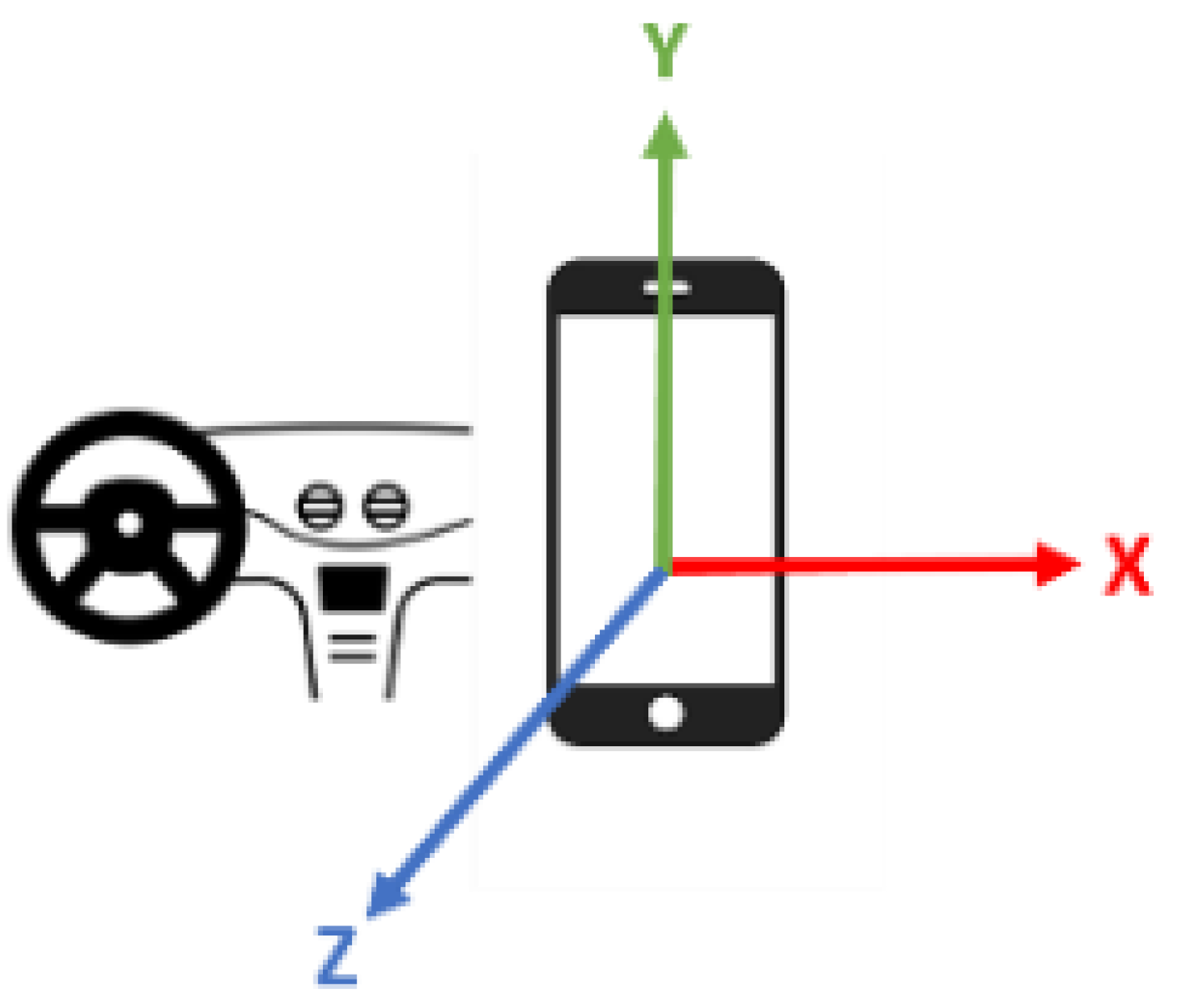
Our research plan will be carried over three steps. First is the stage of the phone app implementation. It consists of developing a smartphone application for data recording. The application will be valid for both iOS and Android phones. The application will allow users to label manually and accurately road segments corresponding to four surface states, namely smooth, bump, potholes, and others. For each labeled segment, the application must record multimodal data describing vehicle accelerations (on three-axis as shown in Figure 1), angular rotations, and geographical positions using the accelerometer, the gyroscope, and the GPS sensors, respectively, of a user’s smartphone. The application will be available for public download shortly. This application will constitute a great tool for researchers to collect in situ labeled data and develop a related machine learning approach.

Using our developed application, the second step of our research is to collect reliable data that will be available and shared on-demand. To automate the road surface inspection, we will explore the best state-of-the-art machine learning models. Validated models on large data will be deployed for real-time scanning and online user alerting. That’s the third step. In this step, a new version of the application will be developed to make it more collaborative. Users will be able to see other user tags and share their labels. This version will be further empowered by trained models deployed for online detection. Please note that this paper covers only the first and the second steps of our research plan. The architecture of the proposed application is described in detail in the next section.

4. Application Architecture and Usage

4.1. Architecture Overview

In this section, we give an overview of the general architecture of the proposed application. The application is called “Road Scanner”. The overall solution architecture is described in Figure 2. Our application is compatible with both iOS and Android smartphones since it is based on cross-platform technology, which is React Native. React Native is a JavaScript-based framework developed by Facebook for cross-platform app development.

To interact correctly with our proposed solution, two interfaces are needed. First the smartphone application and second a dedicated website to visualize and export data. The process of data storage is as follows: once the data are recorded from the mobile sensors (i.e., accelerometer, gyroscope, and GPS), it is initially stored locally on the smartphone. This offline process is useful, especially in the case of a loss of connectivity with the application’s server. Afterward, the application will be continuously synchronizing records with the server to keep the consistency of the data and to ignore any data replication.

Indeed, once the connection is established, the stored data are sent to a remote cloud server called “Road Scanner Server” via specified API calls. All the received data are then saved to a PostgreSQL database. At this stage of the development, to visualize the labeled segment in a map viewer and to export the data, the user needs to access these functionalities via the application’s dedicated website.

4.2. Application Usage

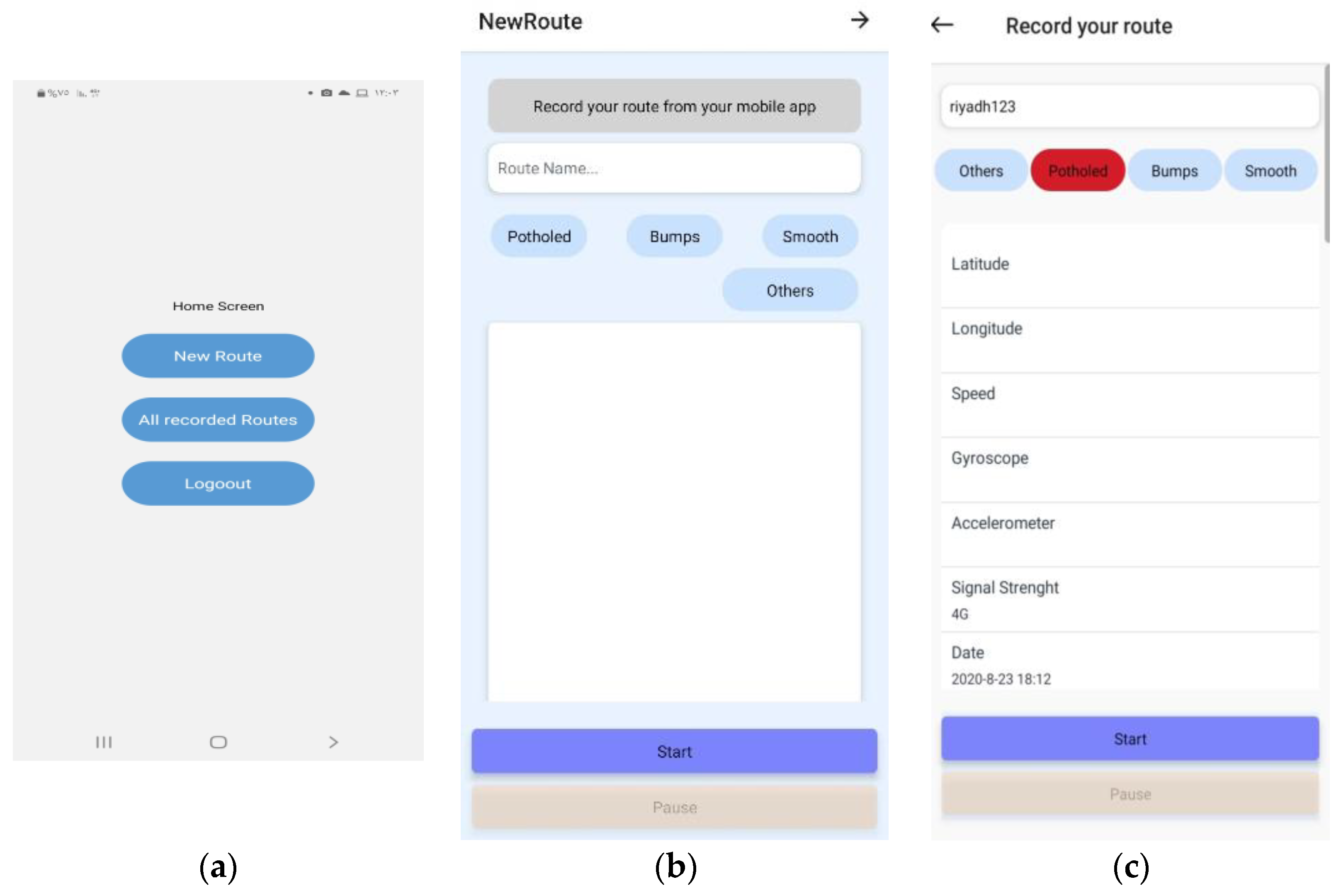
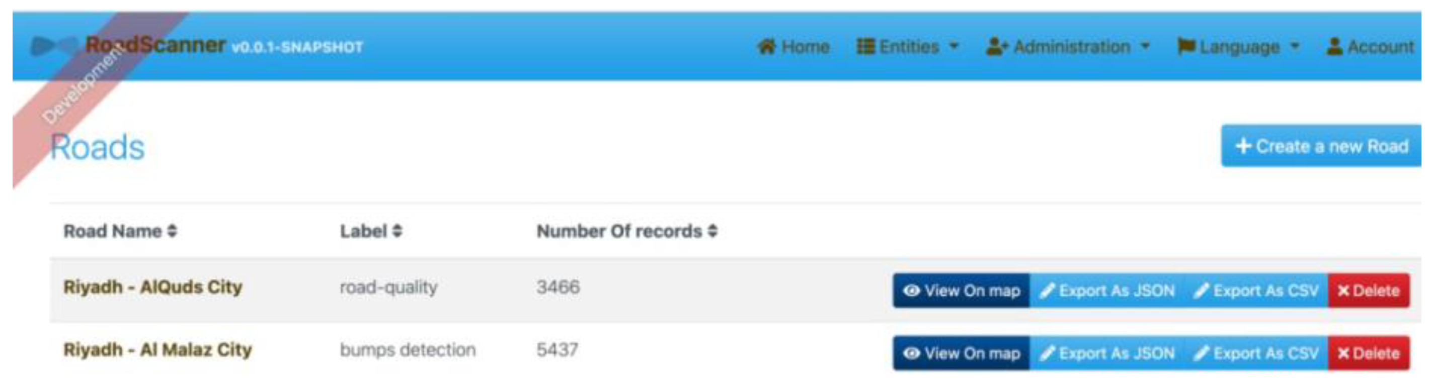
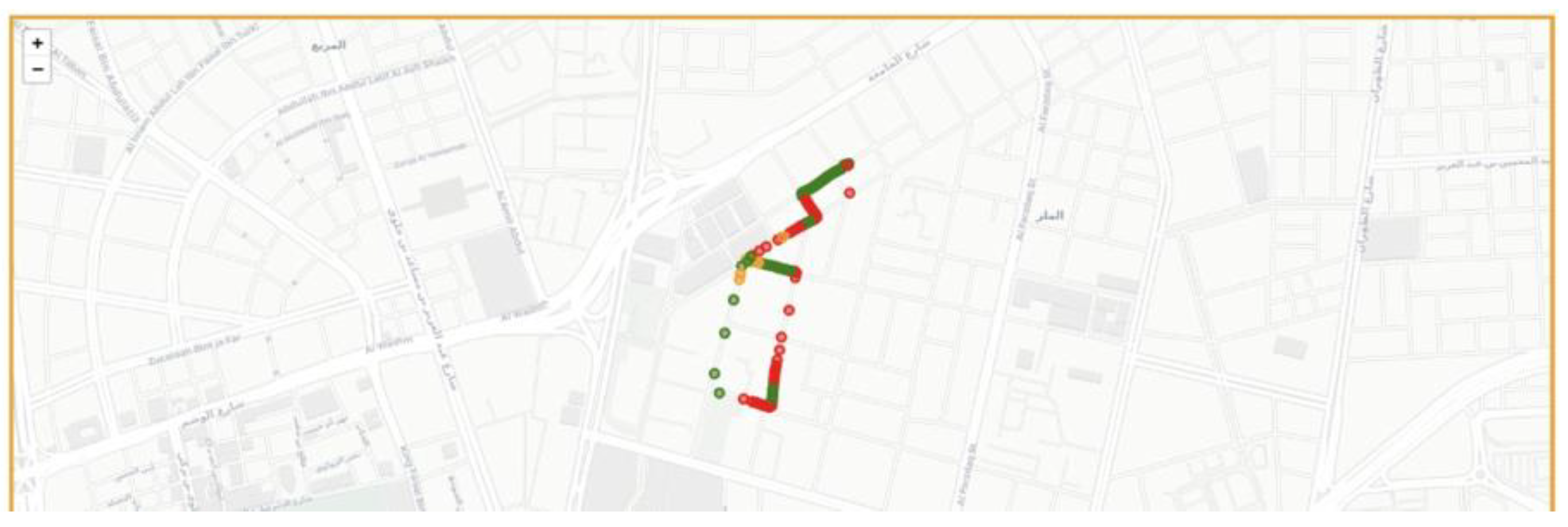
After correctly installing the mobile app, data collection can be launched. The driver has to choose between four labels as shown in Figure 3, which are “Potholed”, “Bumps”, “Smooth”, and “Other”. Note that we can easily switch from one state to another on the same screen to give the experimenter the flexibility of use and recording. In the last stage, the data stored from the mobile phone can be visualized (as shown in Figure 4) and then displayed (as shown in Figure 5) on a map with different colors for easy reading and tracking. This display option is available via the website interface (c.f. Figure 4 and Figure 5). The display function is dotted with a playback feature allowing the researcher to navigate between records on the same road with play, pause, and stop options. Moreover, to analyze or model the stored data, we have provided researchers with the possibility of exporting records either in JSON format or CSV format. The export function is also available via the website interface (c.f. Figure 4). In the next section, we will present the dataset, the classification methods, and the implementation part.

5. Experiments

5.1. Experiments Presentation

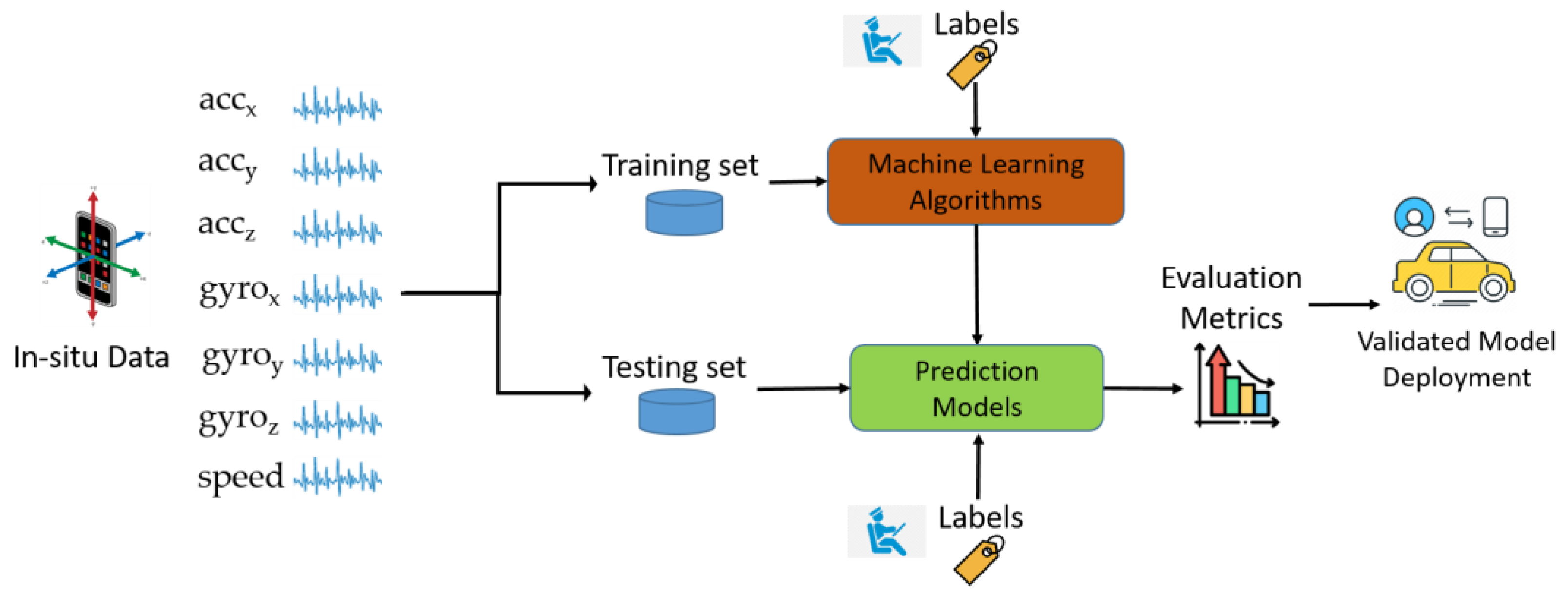
In this section, we introduce the experiment part of our work. As previously mentioned, we aim to train machine learning models to be able to detect road states. To this end, we have built a new dataset containing two types of road status: smooth and potholed. For each labeled segment, multimodal sensorial data were recorded from the accelerometer and the gyroscope of a driver’s smartphone. As shown in

Table 2. A sample of the data used in the experiments.

Speed	acc_x	acc_y	acc_z	gyro_x	gyro_y	gyro_z	Status
13.57	−0.021148682	−0.97845	0.22049	−0.02143	−0.07219	0.047946	smooth
13.57	−0.094284058	−1.04622	0.134445	−0.04775	−0.07095	0.02635	smooth
…	…	…	…	…	…	…	…
8.11	−0.512405396	−0.91891	0.08551	0.496783	0.543487	−0.20743	potholed
8.11	0.346130371	−0.97647	0.704208	0.172343	0.016928	−0.21046	potholed

and Figure 6, a total number of seven features were recorded, namely the 3D accelerometer data (acc_x, acc_y, and acc_z), the 3D angular rotations from the gyroscope (gyro_x, gyro_y, and gyro_z), and the speed of the vehicle. Thus, we aim through machine learning models to map the data from the smartphone sensors to the correct label (smooth or potholed). Technically this problem can be solved by a binary classification approach.

To train our classifiers, a dataset was built using our collected data from our developed application in addition to a richer and larger dataset from the Kaggle website (https://www.kaggle.com/datasets/dextergoes/pothole-sensor-data, accessed on 14 November 2022). Merging the two datasets was a better approach since it makes the trained model more robust and less sensitive to a single smartphone or a single vehicle. The merged dataset contained nearly 1540 samples (1080 for the smooth label, 460 for the potholed label). Moreover, on average, each road sample corresponds approximately to one second of recording, which represents the time granularity of our road segments. Based on this dataset, several classifiers were deeply investigated to obtain the best hyperparameters that give the optimal classification results. From all the tested classifiers, seven classifiers were selected due to their efficient performance in our detection problem. A brief description of these classifiers is given in the next paragraph.

5.2. Classification Models

5.2.1. Artificial Neural Networks

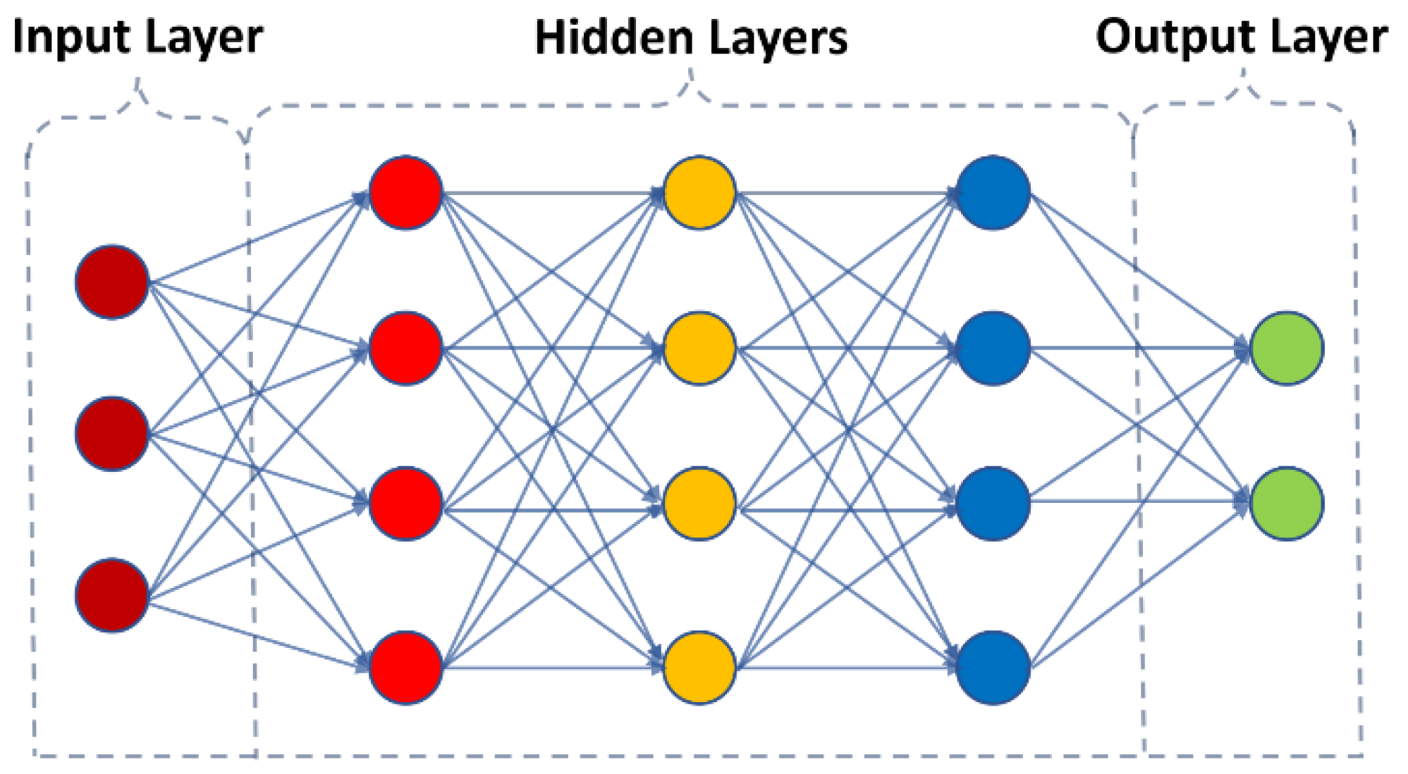
Artificial Neural Networks (ANNs) [23] are computer systems that take their cue from the brain’s biological neural networks. Artificial neurons are the building blocks of an ANN. Similar to brain synapses, these ties carry information between neurons via what we call edges. The signal strength at an edge connection is affected by the weight. Typically, the importance of edges weight shifts as learning progresses. Neurons frequently group into layers. Different layers may modify their inputs in different ways. Signals move through the layers from the input layer (the first layer) to the output layer (the last layer). The ANNs’ main advantages are as follows: (1) it is a self-adaptive data-driven approach, and (2) it is a non-linear model, making it adaptable in modeling real-world problems [24]. The general structure of an ANN is presented in Figure 7.

5.2.2. Support Vector Machines

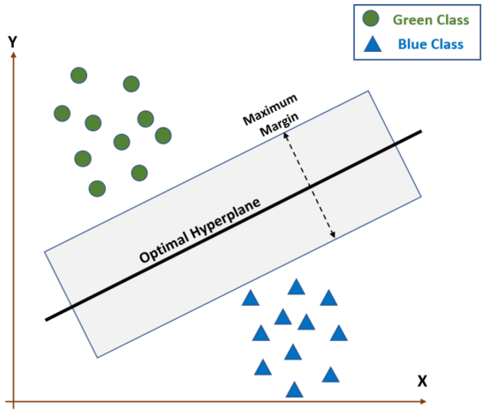
The SVM (Support Vector Machine) [26] is a supervised ML technique that is largely employed for classification. This approach is founded on two fundamental ideas. The first premise is the maximization of the hyperplane’s margin. The objective is to identify the best hyperplane that divides classes by the largest margin. In the case where data are separable in a linear manner, this is a typical quadratic-type optimization issue. Nonetheless, data are frequently linearly inseparable. The kernel function that represents the second essential concept provides the answer by translating the original data space into a higher-dimensional space, where it is probable to obtain a linear separator. The SVM concept handles nonlinear classification problems effectively in this manner [27,28]. An illustration of the SVM Algorithm is shown in Figure 8.

5.2.3. Random Forests

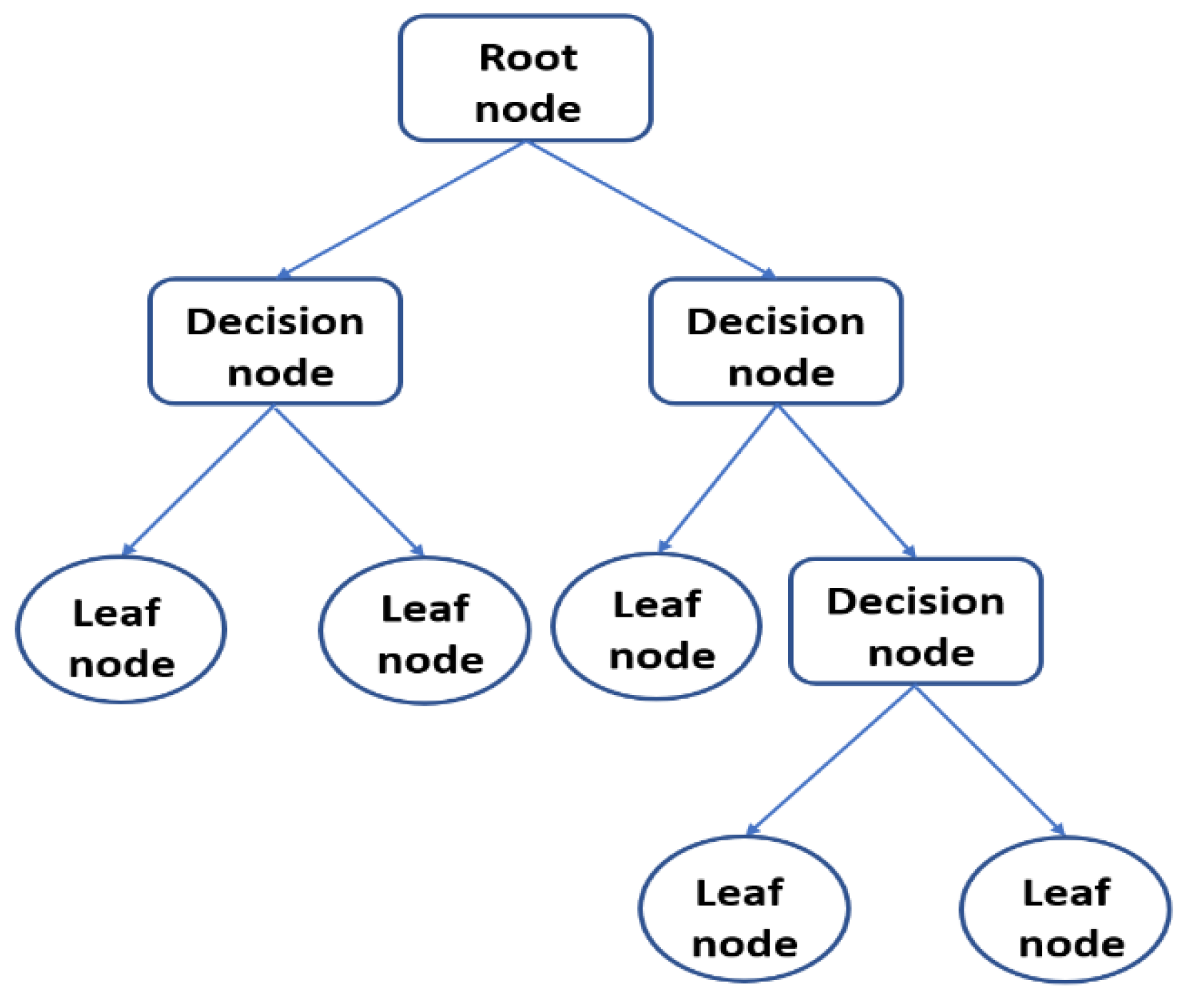
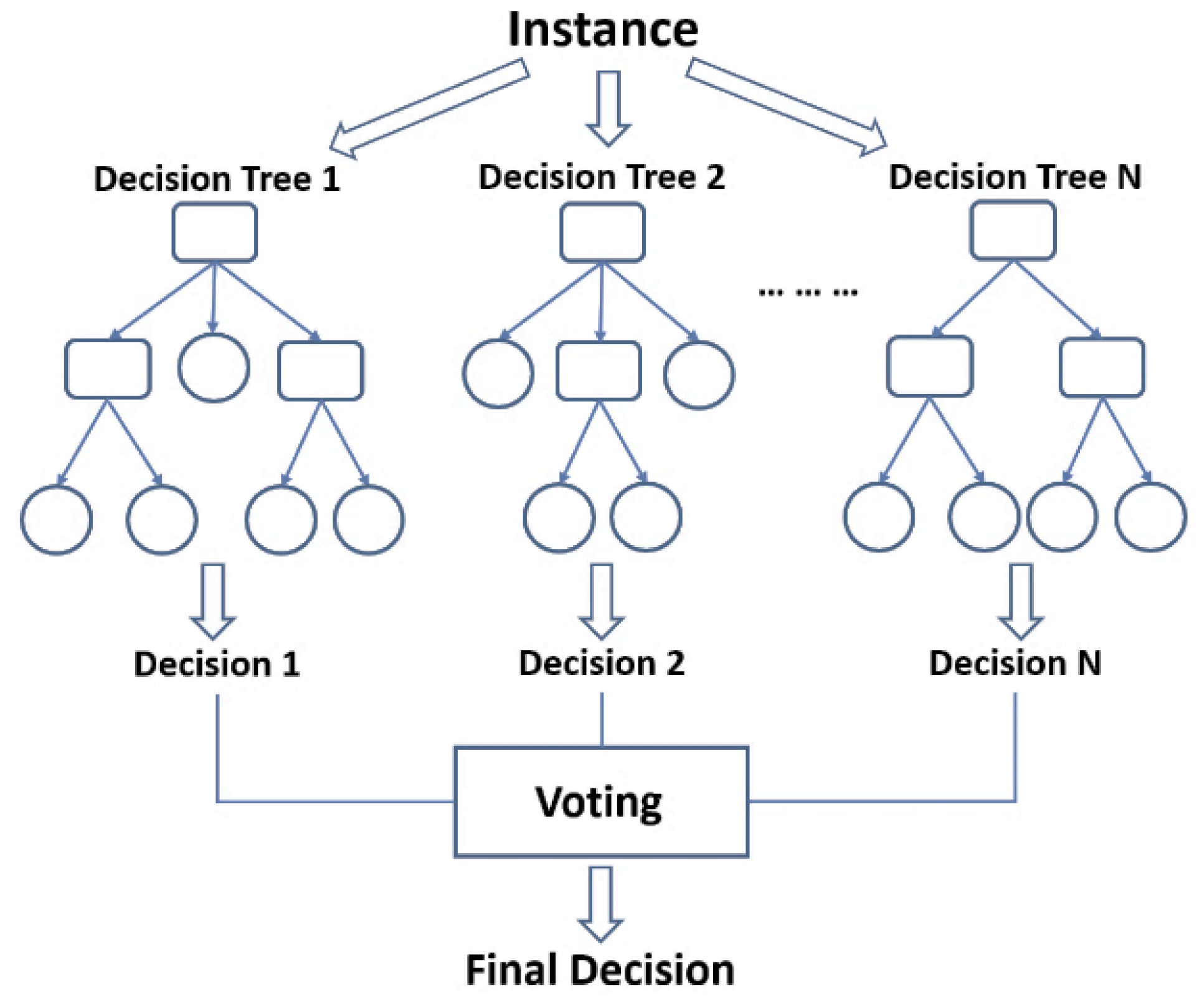
As an ensemble learning technique, random forests (also known as random decision forests) build many decision trees and combine their classification outputs. The output of a random forest is the class chosen by the majority of trees. Among the RF benefits, we can cite: (1) it works well with all types of data, (2) it prevents overfitting issues when compared to decision trees models, (3) it is resistant to noise, (4) it ranks the importance of each variable, and (5) it is a good choice for data imputation and cluster analysis [29,30,31]. The common structure of a Decision Tree is presented in Figure 9 and an illustration of the RF Algorithm is shown in Figure 10.

5.2.4. Extra Trees

Compared to the random forests approach, the major goal of the Extra-Tree approach (an acronym for “extremely randomized trees”) is to further randomize tree building. Instead of trying to identify an ideal cut-point, similar to random forests, this method chooses a cut-point randomly [32]. From a statistical perspective, the cut-point randomization frequently has a beneficial effect on reducing variance. Unlike Random Forest, Extra Trees do not bootstrap observations and do not search for optimum splits [33]. Therefore, several high-dimensional and complicated issues were solved using this approach [34].

5.2.5. Bagging

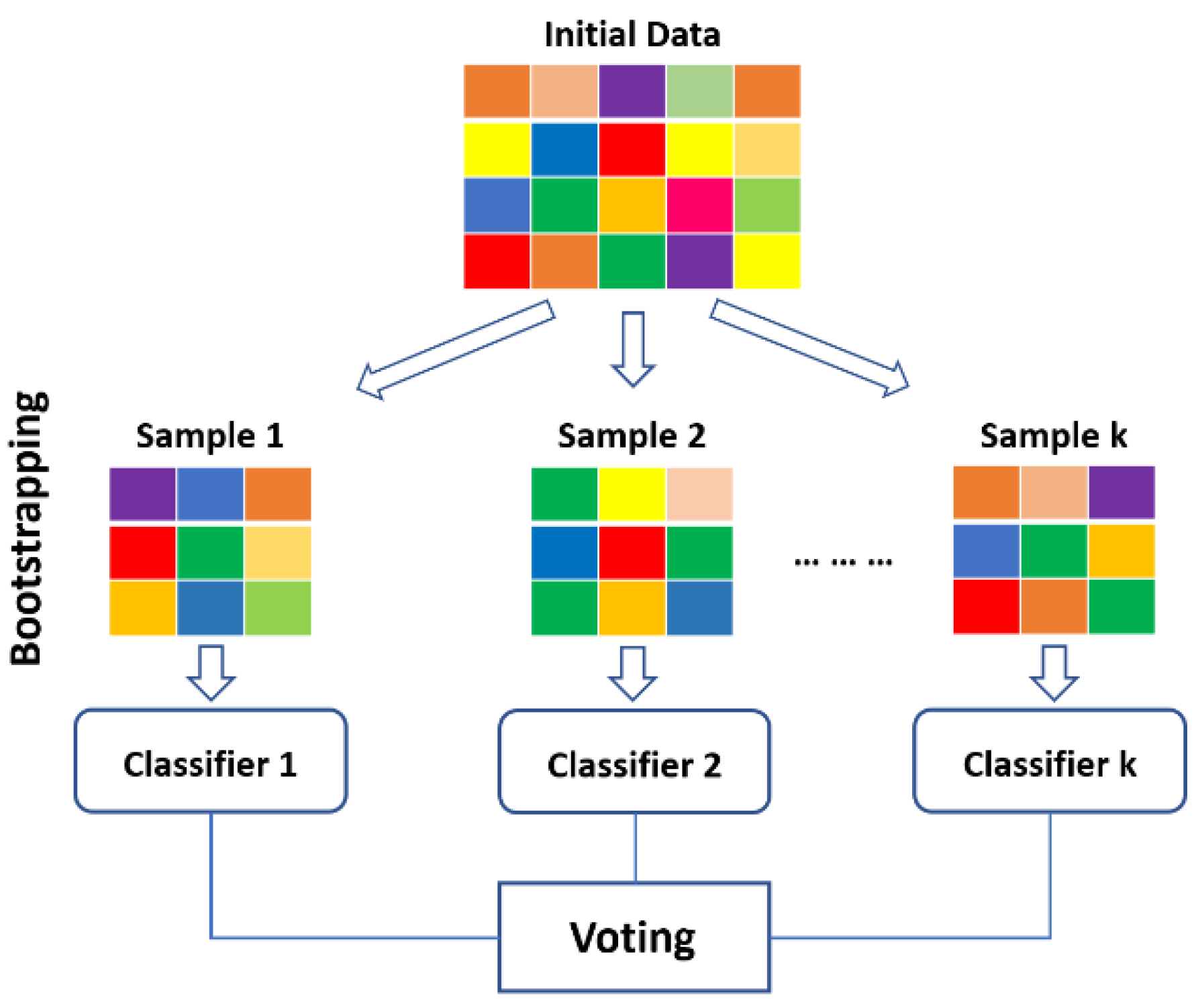
The ML ensemble meta-algorithm called bootstrap aggregating, often known as bagging (from bootstrap aggregating), aims to enhance the stability and accuracy of ML classification algorithms. Additionally, it lowers variance and aids in preventing overfitting [35]. The fundamental concept is to train a variety of models on various randomly chosen subsets of the training data, then combine the predictions of these models using a voting system. It allows to trade off some accuracy for improved resilience, which makes it an attractive solution for many specific problems. An illustration of the Bagging Technique is given in Figure 11.

5.2.6. Gradient Boosting

Gradient Boosting is an ML technique that provides a prediction tool in the form of a collection of relatively weak prediction models, most commonly decision trees [36]. It relies mainly on the boosting technique. The boosting technique begins by fitting the data to a starting model. Then, a second model is constructed that concentrates on properly forecasting instances in which the first model performs badly. It is expected that the combination of these two models will be superior to each model alone. Then, this procedure is repeated several times and every subsequent model aims to address the deficiencies of the boosted ensemble of all preceding models.

5.2.7. Stacking

The process of training a machine learning algorithm that takes as inputs the outputs of several other learning approaches is called Stacking. The combiner algorithm is trained to create a final prediction using all of the predictions of the other algorithms as extra inputs once all of the other algorithms have been trained using the available data. Although in reality a logistic regression model is frequently employed as the combiner, stacking can potentially represent any other efficient model [37,38].

5.3. Evaluation Metrics

In this work, the results of our experiments through the seven selected classifiers (ANN, SVM, Random Forest, Extra Trees, Bagging, Gradient Boosting, and Stacking) are concretely evaluated using five evaluation metrics namely: accuracy, precision rate, recall rate, F-score, and the AUC metric (Area Under Curve). To compute these metrics, we assign the “Positive value” to the smooth class and the “Negative value” to the potholed class. Therefore, the four elements of the confusion matrix are:

• True-Positive (TP) represents the number of instances correctly assigned to the smooth class;
• True-Negative (TN) represents the number of instances correctly assigned to the potholed class;
• False-Positive (FP) represents the number of instances wrongly assigned to the smooth class;
• False-Negative (FN) represents the number of instances wrongly assigned to the potholed class.

The definitions of the evaluation metrics are as follows.

5.3.1. Accuracy

The accuracy metric represents the ratio of the samples that were correctly assigned. Thus, the accuracy of the model is the ratio of all the correct classifier instances over all the classifications. Hence, the higher the accuracy rate, the better the performance of the model. It can be defined as follows:

$$Accuracy=\frac{TP+TN}{TP+TN+FP+FN}$$

(1)

5.3.2. Precision

The precision metric represents the ratio of well-classified samples among all those retrieved for a specific class. For instance, the precision for the smooth class is the ratio of the correctly classified smooth instances (TP) from all the detected smooth instances (TP + FP). It can be defined as follows:

$$Precision=\frac{TP}{TP+FP}$$

(2)

5.3.3. Recall

The recall metric represents the ratio of well-classified samples among all the existing samples for a specific class. For instance, the recall for the smooth class is the ratio of correctly classified smooth instances (TP) from all the existing smooth instances (TP + FN). It can be defined as follows:

$$Recall=\frac{TP}{TP+FN}$$

(3)

5.3.4. F-Score

Since precision and recall are inversely proportional, the F-score (a.k.a F-measure) tries to combine them by computing the harmonic mean of these two metrics. Mathematically, it is defined as follows:

$$F-score=\frac{2TP}{2TP+FP+FN}=2\times \frac{precision\times recall}{precision+recall}$$

(4)

5.3.5. AUC

The Receiver Operating Characteristic (ROC) curve represents a popular evaluation approach for assessing classification efficiency. Indeed, it represents a 2D graph that plots the True Positive ratio on the Y axis and the False Positive ratio on the X axis. Moreover, the greater the Area Under this ROC Curve (also known as the AUC metric), the greater the classification accuracy of the classifier. Therefore, the AUC values range between 0 and 1. On the one hand, a classifier with all false estimations has an AUC value equal to 0, and on the other hand, a classifier with all accurate estimations presents an AUC value equal to 1.

5.4. Implementation

Our experiments were practically computed on a computer dotted with an Intel Core i7-8550 Processor and 16-GB RAM capacity. To limit overfitting issues, a 4-cross validation approach was adopted. In each iteration, 1155 samples were used for training and 385 for testing. Concretely, all models and evaluation metrics were implemented using the python language and well-established data science libraries, such as Pandas, NumPy, and Scikit-learn. For all the models, several hyperparameters were tested and evaluated.

Our empirical tests in finding optimal performances resulted in the following configurations: For ANNs, the best network topology was characterized by two hidden layers (containing each almost 15 nodes), a “relu” activation function, an “adam” solver and an iteration number of 200 for the training process. For The SVM, an “rbf” kernel is adopted and the value of 30 was found to be the best tradeoff for the regularization parameter C. For the Random Forests and the Extra Trees classifiers, the “gini” criterion is adopted and a total number of 100 estimators was empirically validated. Similarly, 100 estimators were used for the Bagging, and the Gradient Boosting classifiers. Particularly for the Bagging, the SVM classifier was found to be the best choice as a base estimator among several other methods. For the Gradient Boosting classifier, the “friedman_mse” criterion was selected as a measure for the split quality, and for the stacking approach, two classifiers were chosen as the best base estimators, namely Decision Trees and SVM. In this latter approach, the final combining estimator was a Logistic Regression classifier. The results of these finely tuned models are presented in the next section.

6. Results and Discussion

The presented results in the following tables (

Table 3. Accuracy results for all classifiers.

Classifier	Accuracy (Standard Deviation)
ANN	86.88 (±1.14)
SVM	88.05 (±1.81)
Random Forest	87.79 (±1.31)
Extra Trees	87.34 (±2.07)
Bagging	86.75 (±0.80)
Gradient Boosting	87.14 (±0.54)
Stacking	86.95 (±0.43)

,

Table 4. F-score results for all classifiers.

Classifier	F-Score (Standard Deviation)
ANN	86.74 (±1.13)
SVM	87.87 (±1.97)
Random Forest	87.43 (±1.30)
Extra Trees	86.65 (±2.37)
Bagging	86.29 (±0.99)
Gradient Boosting	86.69 (±0.49)
Stacking	86.25 (±0.53)

and

Table 5. AUC results for all classifiers.

Classifier	AUC (Standard Deviation)
ANN	91.44 (±1.93)
SVM	91.83 (±1.60)
Random Forest	93.89 (±0.22)
Extra Trees	94.94 (±1.21)
Bagging	92.13 (±1.21)
Gradient Boosting	92.43 (±0.78)
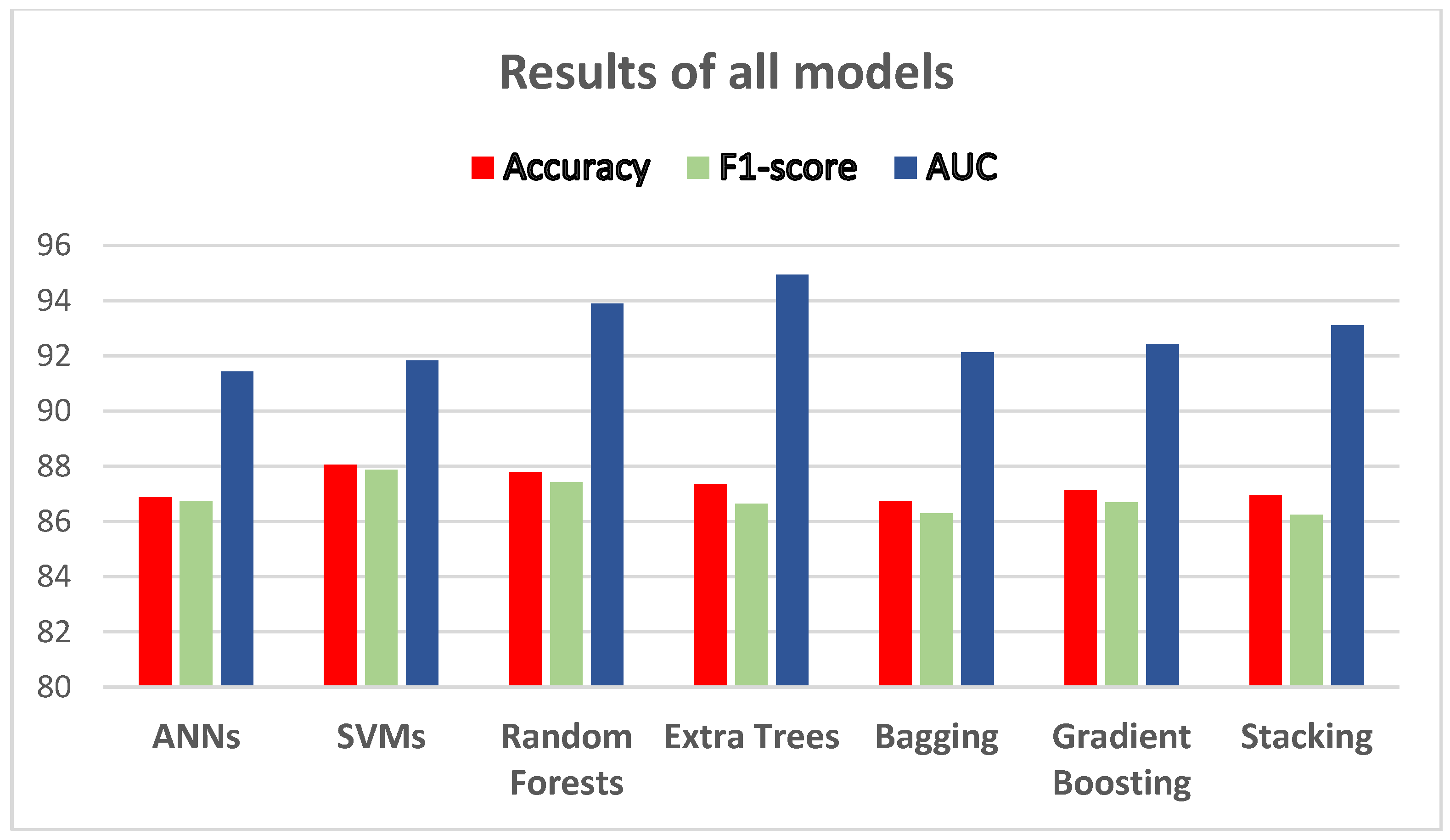
Stacking	93.12 (±0.49)

) correspond to the average metrics (accuracy, F-score, and AUC) followed by the standard deviation, all computed from the four iterations of the cross-validation process. These table results are also summarized in Figure 12.

Taking the accuracy results (Table 3), the best two classifiers were SVM—with an accuracy rate of 88.05%—and Random Forest with an accuracy rate of 87.79%. Similar results were observed for the F-score metric (Table 4). Their respective rates were 87.87% and 87.43%. For the AUC metric (Table 5), remarkable results were given by the Extra Trees classifier (AUC = 94.94%) and the Random Forest classifier (AUC = 93.89%).

In addition, low standard deviation rates were observed for all metrics and all classifiers. For instance, the Random Forests classifier has outputted a standard deviation rate of 1.31, 1.30, and 0.22 for the three measured metrics (Accuracy, F-score, and AUC). Overall, the high average rates and the low standard deviation rates (among all metrics) confirm the good performance of the chosen classifiers.

Moreover, execution times for all the models were also computed. Precisely both training and testing times were calculated as shown in

Table 6. Execution times (training and testing) for all classifiers.

Classifier	Training Time	Testing Time
ANN	6.024	0.002
SVM	1.066	0.073
Random Forest	1.737	0.055
Extra Trees	0.7	0.059
Bagging	46.805	5.776
Gradient Boosting	3.796	0.004
Stacking	5.13	0.101

. For the training part, we notice higher times for ANNs and the non-tree-based ensemble methods (e.g., bagging). For ANNs, this can be explained by the high number of epochs that were needed in the training process. Additionally, because ensemble methods integrate a large number of estimators (e.g., 100 estimators for bagging), the learning step may take a longer time, especially for the non-tree-based models. For the testing part, all models (except bagging) present great performances, which is suitable for the deployment of these models in real-time applications.

Furthermore, for a better understanding of the results, we have also computed the confusion matrix of the SVM classifier, which has shown the best performance in terms of Accuracy and F-score. The confusion matrix is shown in

Table 7. Confusion matrix of the SVM classifier.

Accuracy = 88.05		Predicted
		Smooth	Potholed
Actual	Smooth	1007	73
	Potholed	111	349

.

On the one hand, the model has succeeded to detect 1007 instances (TP) among the 1080 instances of the smooth class. On the other hand, 349 instances (TN) were correctly detected among the 460 instances of the potholed class. From these confusion matrix statistics, per-class metrics were computed as shown in

Table 8. Results per class for the SVM classifier.

Class	Precision	Recall	F-Score
Smooth	90.07	93.24	91.63
Potholed	82.70	75.87	79.14

. These per-class metrics are mainly Precision, Recall, and F-score.

Taking the smooth class, the detection rates are significantly higher than those of the potholed class. For instance, the precision rate of the smooth class is 90.07% versus 82.70% for the potholed class. The difference is much larger for the Recall metric as the smooth class recorded 93.24% versus only 75.87% for the potholed class.

Indeed, the classifiers seem to be accurate and precise when detecting a certain class since both precision rates are relatively high. However, the classifiers seem to have more difficulties in recalling the totality of the potholed-class instances. This confusion may be caused by the speed dependency problem [39]. Actually, when a vehicle crosses a pothole at various speeds, the captured signal by the accelerometer will have a variable amplitude which may confuse the trained classifiers. This issue may be overcome in the future by increasing the sampling rate when recording the potholed segments. Higher sample rates deliver more data per second, which enhances recognition rates.

Another limitation of our work and which represents a challenge, is the accuracy and precision of the smartphone sensors themselves. It differs depending on the brand, the specifications, and the quality of the smartphone; therefore, appropriate preprocessing operations should be applied to filter the possible noises related to the sensing process.

In addition to this, a car’s suspension quality can also affect the sensing accuracy and precision.

Moreover, although we prepared our smartphone application to record four types of segments, we could not collect enough data for the ‘bumps’ and ‘other’ classes. Therefore, we had to omit the aforementioned classes due to the concern that their inclusion might compromise the validity of the machine learning-based models.

7. Conclusions

In this study, we described the “Road Scanner” route application, which enables onboard users to distinguish between four different types of road segments: smooth, bumpy, potholed, and others. The application uses the accelerometer, gyroscope, and GPS integrated into smartphones to record multimodal data for each tagged segment. A dataset was gathered and combined with other online datasets to serve as a comparison for the classification methods in order to evaluate the application. In fact, a number of machine learning models were used to map the sensors-data that were gathered to the appropriate route state. Python and well-known data science tools were used to implement all models and evaluation criteria. SVM and Random Forest were the top two classifiers. The Extra Trees classifier and the Random Forest classifier produced excellent outcomes for the AUC metric. Additionally, all measures and all classifiers showed low standard deviation rates. Overall, the high average rates and the low standard deviation rates (across all metrics) attest to the chosen classifiers strong performance.

Future work will involve increasing the sampling rate when recording the potholed segments in order to address the speed dependency issue that was previously mentioned. Additionally, the future edition will be enhanced by machine learning models that are deployed online to provide real-time notifications regarding various road surface conditions, which represents a challenge because of the problem of sensor qualities and precision that varies depending on a smartphones brand and specifications; a challenge that we are willing to face by developing appropriate noise filters for use with different smartphones sensor specifications. Furthermore, we are willing to include the actual excluded classes ‘bumps’ and ‘other’ by focusing on road areas that will permit us to record sufficient data. We will also attempt to use formal verification techniques to validate the different steps of the proposed approach [40]. The security challenges related to the use of our application need to be considered as well [41,42]. Our application may be also extended in order to cover other aspects and needs in our modern smart societies, cities, and homes [43,44].