Abstract
The novelty of this paper is to propose a numerical method for solving ordinary differential equations of the first order that include both linear and nonlinear terms (ODEs). The method is constructed in two stages, which may be called predictor and corrector stages. The predictor stage uses the dependent variable’s first- and second-order derivative in the given differential equation. In literature, most predictor–corrector schemes utilize the first-order derivative of the dependent variable. The stability region of the method is found for linear scalar first-order ODEs. In addition, a mathematical model for boundary layer flow over the sheet is modified with electrical and magnetic effects. The model’s governing equations are expressed in partial differential equations (PDEs), and their corresponding dimensionless ODE form is solved with the proposed scheme. A shooting method is adopted to overcome the deficiency of the scheme for solving only first-order boundary value ODEs. An iterative approach is also considered because the proposed scheme combines explicit and implicit concepts. The method is also compared with an existing method, producing faster convergence than an existing one. The obtained results show that the velocity profile escalates by rising electric variables. The findings provided in this study can serve as a helpful guide for investigations into fluid flow in closed-off industrial settings in the future.
1. Introduction
Advancement in flow-saturating porous medium revealed its applications in several mechanical and biochemical industries. These may include medicines, heat exchangers, insulation of optic fiber, hydrocarbon recovery, geothermal energy systems, wood drying, ecosystem regulation, geophysics, and catalytic reactors. As a result of the perforated medium flow, there was a complicated interplay among the liquid, the fragments, the column wall, and the sorting particles.
Darcy’s law is experienced when there is a reduced velocity of liquid and low porosity condition of medium. However, it is worth mentioning that this law becomes ineffective when high velocity and inappropriate pores are present in a medium. The non-Darcian model overcomes the limitations of Darcy’s law by allowing for the generation of tortuosity inertial drag hits, vortex diffusion, and other phenomena by modifying the Darcian relation. To improve Darcy’s model, Forchheimer uses the velocity-squared term in the momentum expression (also known as Forchheimer’s extension) to do the job [1,2].
Pal and Mondal [3] investigated non-Darcy Forchheimer flow with Dufour and Soret effect over a permeable surface. Hydrodynamic, mixed convective, non-Darcy flow with changing characteristics and temporal dependence was explained by Pal and Mondal [4]. Muhammad et al. [5] explained the Cattaneo–Christove double diffusion model for Darcy-Forchheimer flow as represented by the exponentially bent stretched sheet. Sajid et al. [6] investigated the Darcy–Forchheimer radiative flow of Maxwell fluid, while Khan et al. [7] investigated the Darcy–Forchheimer carbon nanotube flow with entropy rate between spinning disks. Details regarding Darcy–Forchheimer flow can be seen in reference [8].
Various engineering fields have introduced the entropy optimization phenomenon, which produced significant results in the thermal management system. It can calculate the irreversibility of a system with fluid friction, heat and solute transport, molecular vibration, thermal radiation, the Joule–Thompson effect, and other non-ideal processes. It is a considerable fact that reducing the entropy rate substantially improved the efficiency of closed systems, such as power plants, heat exchangers, fuel cells, geothermal energy systems, engineering phenomena, thermal storage, and advanced nanotechnology. Bejan was a pioneer who introduced entropy generation in convective flow [9,10]. Entropy generation details can be seen in [11,12].
Muskal [13] coined the term non-Darcy model as Forchheimer. Massive application of the moment of fluid flow over a permeable surface in technical, biological, and scientific domains, such as artificial dialysis, gas turbines, atherosclerosis, catalytic converters, and geo-energy generation, has multiplied its value by a factor of ten. The 2-D Darcy–Forchheimer flow of a non-Newtonian liquid with varying characteristics was first seen by Hayat et al. [14]. In contrast, the convective flow of a Darcy–Forchheimer liquid with a varying heat sink or source and viscosity was explored by Pal and Mondal [15]. Mallawi and Ullah [16] instead studied the effect of a magnetic dipole on the reactive flow of Darcy–Forchheimer Carreau nanomaterial and found evidence of non-uniform heat conductivity. The convective flow of a Darcy–Forchheimer hybrid nanomaterial subject to a cubic autocatalysis chemical reaction was the focus of research by Alshomrani and Ullah [17]. However, Seth and Mandal [18] addressed how the hydromagnetic effect can redirect a stream of Darcy–Forchheimer Casson liquid into a void. An elicit publication on the porous medium is discussed in [19,20,21,22].
Thermal and solute transportation across permeable surfaces has attracted researchers’ attention during the last two decades. The Dufour effect in liquid was studied by Rastogi and Madan [23]. As time passed, researchers examined the effects of diffusion and temperature on a homogeneous mixture [24,25]. The convective flow of a liquid with a non-uniform viscosity subject to a permeable material was investigated by Moorthy and Senthilvalivu [26]. El-Arabawy [27] briefly discussed the non-uniform temperature in a convective fluid flow responsive to thermal diffusion and diffusion-thermo effects.
Refs. [28,29,30,31,32] were the reviews with references that reflect the relevant title. Buonomo [33] provided an entropy analysis of a water-based hybrid nano liquid subject to mixed convection. Khan et al. [34] investigated irreversibility in the dissipative flow of nanomaterial with melting and radiation over a stretching sheet. Few studies of the entropy rate are cited in [35,36,37,38].
MHD is related to a phenomenon in which the combined effect of velocity and magnetic fields is studied. Each unit volume of electrically conducting fluid having MHD is called a Lorentz force that acts opposite to the direction of velocity. MHD flow has applications in astrophysics, MHD flow meters, MHD generators, ship propulsion, MHD flow control, magnetic filtration and separation, jet printers, and fusion reactors. The electrical MHD flow has been investigated by [39] over the permeable stretching sheet using the Buongiorno model. The governing equations of electrical MHD flow have been expressed in partial differential equations. Later, those governing equations were reduced into nonlinear differential equations and tackled with the implicit finite difference method. The phenomenon of electrical MHD flow over the sheet has been addressed in [40] using the effects of Joule heating, chemical reaction, and viscous dissipation. The governing equations have been reduced to a set of ordinary differential equations and solved by numerical method. The results showed that velocity and temperature profiles were by escalating electric field while the concentration profile declined. The combined effects of electrical and magnetic fields over the fluid flow have also been considered in [41].
Numerical methods can be thought of as a tool to solve problems in science and engineering. Since the exact solution of every differential equation is impossible, some approximate method can be considered to handle this issue. In literature, some analytical methods exist to find the solution of differential equations in infinite series. The series comprise exponential, polynomial, trigonometric, or combinations of these functions. The approximate analytical methods may produce exact solutions to some problems. Still, for highly nonlinear problems, some infinite series of the solution is truncated, and these finite components can be used for further processing. Some of these analytical methods find the solution valid only on a small domain if only a few components of the solution series are considered. The computation time for analytical methods is more than for some numerical methods. The numerical methods use numerical values instead of analytical functions, leading to computation time decay. Most analytical methods do not divide the whole domain into small subdomains, but in some of the existing numerical methods, the whole domain is divided into a small finite number of intervals or subdomains. In addition, different numerical methods give low- and high-order accuracy and different lengths of stability regions. So, an appropriate numerical method can be chosen to solve the given problem. The proposed numerical method is a two-stage or predictor–corrector method that uses the information to find the second-order derivative of the dependent variable in the given first-order differential equation. The method is applied to the system of boundary value problems that arise in the flow over-the-sheet phenomenon. The method requires first-order differential equations, so second and third-order boundary value problems are reduced into a system of first-order differential equations with given and supposed initial conditions. Later on, the supposed initial conditions are found using the shooting approach. So, the shooting method based on the proposed method with an iterative method is applied to the considered problem.
2. Proposed Numerical Scheme
The proposed numerical scheme is a two-stage scheme. Both stages of the scheme are implicit. The first stage comprises the information on first- and second-order derivatives of dependent variables in the given differential equation. In the beginning, the procedure of constructing a scheme considers a differential equation
Subject to the initial condition
where is a constant.
The first stage of proposing a scheme is to find the solution at an unknown time level. Let it be described as
This second stage (3) can be extended from the Backward Euler method. In this stage (3), denotes the step size, which can be expressed as , where the domain for the solution of (1) is represented as and denotes the number of total time levels.
Three unknown parameters formed the second stage. Using the Taylor series expansion, the unknown values of three parameters can be determined. The second stage of the proposed scheme is as follows:
where “”, and “” are three unknown parameters. Expanding and using the Taylor series, it is obtained:
Substituting Equation (3) into Equation (5) yields
Expanding and using Taylor series expansion yields
Comparing coefficients of and on both sides of Equation (7), it is obtained
By solving Equations (8)–(10), the values of the unknown parameters are obtained as
Thus, the first and second stages of the proposed scheme for discretizing Equation (1) can be expressed as
where and
2.1. Stability Analysis
A linearized or linear equation is considered for finding the stability region of the proposed scheme. To do so, let the equation be expressed as
Applying the first stage of the proposed scheme on Equation (14) yields
The second stage for discretizing Equation (14) can be expressed as follows:
Substituting Equation (15) into Equation (16) gives
where
Equation (17) can be re-arranged as
The stability region for the proposed scheme, when applied to Equation (14), is expressed as
So, the scheme will remain stable if it satisfies inequality (19). The appropriate values of and can be chosen to obtain a stable solution.
2.2. Stability Analysis for System of Equations
The system of linear or linearized first-order differential equations can be expressed in a single vector matrix of the form
The first or predictor stage of the scheme for the solution of Equation (20) can be expressed as
The second or corrector stage of the scheme for the solution of Equation (20) is given as
Since the proposed scheme is implicit in solving difference Equations (21) and (22), an iterative scheme is employed. Therefore, applying the Gauss–Seidel iterative method to Equation (21) is obtained
Similarly, Equation (22) is re-written as
The Fourier series or Von Neumann stability analysis is employed to check the proposed scheme’s stability conditions. To do so, consider the following transformations:
where
Substituting some of the relevant transformations from (25) into Equation (21) yields
Simplifying Equation (26), it is obtained:
Similar to the predictor substituting relevant transformation from Equation (25) into Equation (24), the resulting equation is given by
Upon simplifying Equation (28), it leads to
Inserting Equation (27) into Equation (29) gives
Re-write Equation (30) as
The stability can be expressed as
where is the identity matrix.
3. Examples: Electrical MHD Flow
Consider steady two-dimensional, incompressible, and laminar electrical MHD Casson nanofluid flow over the sheet. Let the sheet be moved along the positive -axis, where -axis is placed along the sheet. The -axis is placed perpendicular to the sheet. The bottom layer of the fluid coincides with the sheet. Let the sudden movement of the sheet with velocity generate the flow . Effects of Darcy–Forchheimer’s characteristics, thermal radiation, and viscous dissipation are also considered. Under the boundary lawyer assumptions and by following [42], the governing equations of the flow are expressed as
Subject to the boundary conditions:
where and are, respectively, horizontal and vertical components of velocity. and are, respectively, temperature and concentration of fluid; and are, respectively, temperature and concentration at the sheet; and are, respectively, temperature and concentration away from the sheet; is kinematic viscosity; is the Casson parameter; represents electrical conductivity; is the density of the fluid; and are, respectively, strength of magnetic and electrical fields; represents mean absorption coefficients; is a non-uniform inertia coefficient; is thermal diffusivity; is the dynamic viscosity; is the specific heat capacity; is the Brownian diffusion coefficient; represents thermophoresis coefficient; is the reaction rate parameter; is the Stefan–Boltzmann constant; and is the mean absorption coefficient.
For reducing Equations (33)–(37) to corresponding dimensionless form, consider the following transformations:
Upon substituting transformation (38) into Equations (33)–(37), it yields
Subject to the dimensionless boundary conditions:
where is the magnetic parameter, is electric field parameter, permeability of the porous medium, is the Forchheimer number, is the Prandtl number, is Eckert’s number, is the Brownian motion variable, is the thermophoresis variable, is the radiation parameter, is the Schmidt number, and is the reaction rate, and these are defined as
4. Numerical Procedure
The proposed numerical scheme can be applied to solve first-order differential equations. Since Equations (39)–(41) are more than first-order ODEs, these ODEs Equations (39)–(41) will be converted into first-order ODEs as follows:
By employing the first stage of the proposed scheme on Equations (43)–(49), it yields
where and
where and
Now applying a second stage of the proposed scheme on Equations (43)–(49), it is obtained:
where
The skin friction coefficient, local Nusselt number, and local Sherwood number are defined as
where
By applying transformations (38), dimensionless forms of skin friction coefficient, local Nusselt, and local Sherwood numbers are expressed as
where denotes the Reynolds number.
5. Results and Discussions
5.1. Numerical Technique
The proposed scheme is employed for solving a system of boundary value problems. The scheme is comprised of two stages. The first stage requires the computation of the second-order derivative of the dependent variable. Since the proposed scheme combines implicit and explicit computations of terms, an iterative procedure is also employed for solving difference equations obtained by applying the proposed scheme. The iterative procedure finds the solution to the problem using an initial guess. The iterative procedure will stop if the given criterion is met. This criterion is based on the maximum of norms for the difference of solutions computed at two consecutive iterations. If this maximum of norms is less than some given tolerance, the iterative procedure will be stopped. Otherwise, it continues to find solutions iteratively. The solution at the next iteration is found by the information of the solution found at the previous iteration. The solution convergence also depends on the guess choice for Matlab solver fsolve. Since the proposed scheme finds the solution of only first-order differential equations, some strategy is adopted for solving the second- or high-order differential equations with boundary conditions. For this case, a shooting approach is considered. The shooting method is based on the proposed scheme for solving given ODEs, an iterative method for solving difference equations, and a Matlab solver fsolve for solving equations. A procedure is applied for solving second- and third-order differential equations that reduce these equations into first-order differential equations. However, this procedure also requires an initial condition for each first-order equation in the system. Since the given problem is a boundary value, unknown initial conditions are assumed at the leftmost boundary of the domain for those boundary conditions implemented on the rightmost boundary of the domain. The Matlab solver fsolve uses an initial guess for unknown initial conditions and finds the solution with given estimated initial conditions. The solver fsolve continues its iterative procedure until the residuals of boundary conditions tend to zero. The range of physical parameters depends on the convergence of the proposed scheme. So, any numerical value of parameters can be chosen if the scheme provides a stable solution. In addition, the numerical values of the parameter(s) depend on the considered case of fluid. So, if a particular fluid is chosen, corresponding values of parameters will then be checked to find a stable solution. The stability and convergence of the solution also depend on the step size. These types of numerical schemes have not been discussed widely in the literature. Mostly in existing schemes, first-order derivatives of the dependent variable are considered, but the proposed schemes considered the information of the second-order derivative of the dependent variable. So far, the scheme has the advantage of having third-order accuracy and faster convergence compared with the existing first-order Euler scheme.
5.2. Velocity Profile
Equations (39)–(42) are solved with the proposed strategy of a numerical scheme, a Matlab solver, and an iterative method. Figure 1 shows the convergence of two different employed numerical schemes. The first-order implicit Euler method and proposed scheme are applied to solve the considered differential Equations (39)–(42). Figure 1 shows that the proposed scheme converges faster than an existing first-order scheme for finding the maximum of norms. The first-order Euler method requires fewer computations than the proposed scheme, which is one of the advantages of using the Euler method. Figure 2 deliberates the effect of the Casson parameter and an electric variable on the velocity profile. The velocity profile is declined and boosted by the rising Casson parameter and electric variable, respectively. Since an increment in the Casson parameter reduces the diffusion coefficient, this slows down the spreading procedure of molecules in the fluid flow, and, therefore, velocity tends to decay. The effect of the porosity parameter and inertia coefficient on the velocity profile is displayed in Figure 3. The velocity profile is declined by enhancing the porosity parameter and inertia coefficient. An increment in the porosity parameter produces resistance to the velocity of the flow, and, therefore, velocity declines. The growth in the inertia coefficient gives rise to the drag force, resulting in the decay of the velocity profile.

Figure 1.
Convergence of two schemes using
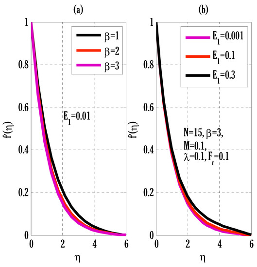
Figure 2.
Variation of Casson parameter and electric variable on velocity profile using
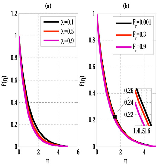
Figure 3.
Variation of porosity parameter and inertia coefficient on velocity profile using
5.3. Temperature Profile
Figure 4 displays the effect of the Eckert number and radiation parameters on the temperature profile. Growth in both parameters offers enhancement in the temperature profile. Since friction between fluid particles rises due to escalation in the Eckert number and heat flux also rises due to incoming radiations, this increases the temperature profile. Figure 5 shows the temperature profile with a variation of the Brownian motion parameter and Biot number, that is, temperature profile augmentations by incrementing the Brownian motion parameter and Biot number. Since the escalation of random movement of particles spreads the hot particles in the plate’s vicinity, this leads to temperature profile growth.
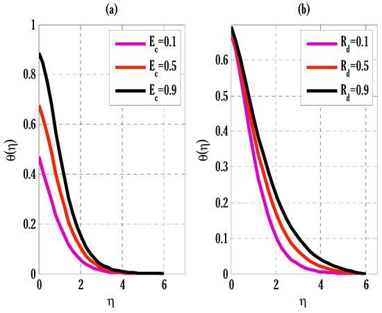
Figure 4.
Variation of Eckert number and radiation parameter on temperature profile using

Figure 5.
Variation of Brownian motion parameter and Biot number on temperature profile using
5.4. Concentration Profile
The effect of thermophoresis and Brownian motion parameters on the concentration profile is depicted in Figure 6. The concentration profile grows and declines by, respectively, rising thermophoresis and Brownian motion parameters. The rise in thermophoresis forces transfers particles from the plate to its vicinity, leading to a rise in the concentration profile. The variation of the Schmidt number and reaction rate parameters on the concentration profile is displayed in Figure 7. By looking at this Figure 7, it can be deduced that the concentration profile decays by escalating the Schmidt number and reaction rate parameter. The decay in the concentration profile due to the increment in the Schmidt number is the consequence of the decline in the mass diffusivity that slows down the diffusion process, resulting in a decline in the concentration profile. The enhancement in the reaction rate parameter produces breaking and forming of new substances, which slows down the concentration profile.
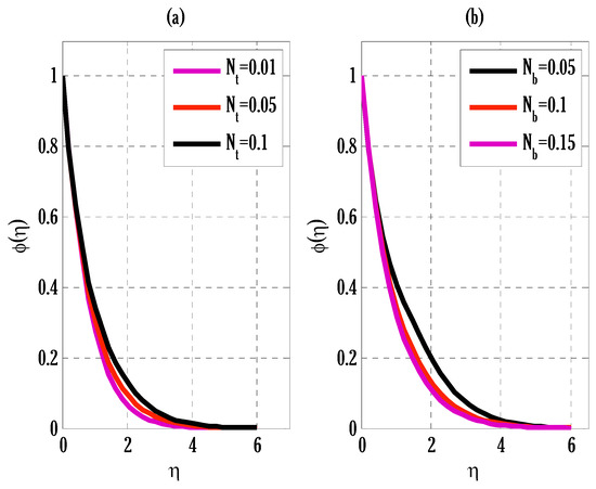
Figure 6.
Variation of thermophoresis and Brownian motion parameters on concentration profile using
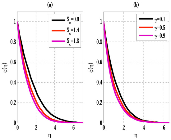
Figure 7.
Variation of Schmidt number and reaction rate parameter on concentration profile using
5.5. Skin Friction Coefficient, Local Nusslt, and Sherwood Numbers
Table 1 compares some results of the proposed scheme with those given in past research. The agreement of numerical values obtained in this research with those in past research can be seen, and this also verifies the Matlab code used for the computations performed in this research. Table 2 shows the numerical values of skin friction coefficient (excluding the Reynolds number) by varying the electric variable, Casson parameter, magnetic parameter, and inertia coefficient. The skin friction coefficient decays by the rising electric variable and escalates by enhancing values of the Casson parameter, magnetic parameter, and inertia coefficient. Table 3 displays the numerical values of the local Nusselt number (excluding the Reynolds number) with a variation of the thermophoresis parameter, Brownian motion parameter, Prandtl number, and Eckert number. The local Nussult number decays by increasing the thermophoresis parameter, Brownian motion parameter, and Eckert number, and it grows by rising values of the Prandtl number. The effect of the thermophoresis parameter, Brownian motion parameter, Schmidt number, and reaction rate parameter on the local Sherwood number (excluding the Reynolds number) is given in Table 4. The local Sherwood number declines by growing the Brownian motion parameter, whereas it escalates by increasing the thermophoresis parameter, Schmidt number, and reaction rate parameter.

Table 1.
Comparison of the proposed scheme with past research for finding numerical values of using
Table 2.
List the numerical values of using
Table 3.
List the numerical values of using
Table 4.
List of the numerical values of using
6. Conclusions
A third-order scheme has been proposed for solving first-order ODEs. The theoretical stability region of the scheme has been found when applied to linear scalar ODE. The scheme has been employed for a dimensionless mathematical model obtained from the boundary layer nanofluid flow phenomenon over the flat plate. Since the scheme is implicit, an iterative method is also considered to solve the difference equations obtained by applying the proposed scheme to the considered set of ODEs.
Various partial differential equations encountered in the sciences and engineering can be solved using the proposed numerical scheme. Following the completion of this study, it is possible to propose alternative applications for the current methods in addition to the current uses [45,46,47,48]. In addition, the proposed method is intuitive and may be applied to the solution of a broader class of partial differential equations in science and engineering. From the obtained results, the following points can be concluded:
- The scheme provided faster convergence than an existing implicit Euler method.
- The scheme also provided third-order accuracy, whereas the implicit Euler is first-order accurate.
- The velocity profile decayed and grew by raising the Casson parameter and electric variable values, respectively.
- The Brownian motion parameter and Biot number were increased to increase the temperature profile.
- The concentration profile was raised and decayed by rising thermophoresis and Brownian motion parameters, respectively.
- The concentration profile declined by augmenting the Schmidt number and reaction rate parameter.
Author Contributions
Conceptualization, methodology, and analysis, writing—review and editing, Y.N.; funding acquisition, K.A.; investigation, Y.N.; methodology, M.S.A.; project administration, K.A.; resources, K.A.; supervision, M.S.A.; visualization, K.A.; writing—review and editing, M.S.A.; proofreading and editing, M.S.A. All authors have read and agreed to the published version of the manuscript.
Funding
The authors would like to acknowledge the support of Prince Sultan University for providing the Article Processing Charges (APC) of this publication.
Institutional Review Board Statement
Not applicable.
Informed Consent Statement
Not applicable.
Data Availability Statement
The manuscript includes all required data and implementing information.
Acknowledgments
The authors wish to express their gratitude to Prince Sultan University for facilitating the publication of this article through the Theoretical and Applied Sciences Lab.
Conflicts of Interest
The authors declare no conflict of interest.
Nomenclature
| Horizontal and vertical components of velocity | Electrical conductivity of the fluid | ||
| Cartesian coordinates | Temperature of fluid | ||
| Kinematic viscosity | Temperature of fluid at wall | ||
| Density of fluid | Ambient temperature of the fluid | ||
| Concentration of fluid | Concentration on the wall | ||
| Brownian diffusion coefficient | Ambient concentration | ||
| Specific heat capacity | Thermophoresis coefficient | ||
| Strength of electric field | Strength of imposed transverse magnetic field | ||
| Permeability of porous medium | Thermal diffusivity | ||
| Reaction rate parameter | Drag coefficient | ||
| Mean absorption coefficient | Stephan–Boltzmann constant | ||
| Casson parameter | Dynamic viscosity | ||
| Magnetic parameter | Electric field | ||
| Forchheimer number | Permeability of the porous medium | ||
| Brownian motion variable | Thermophoresis variable | ||
| Radiation parameter | Schmidt number | ||
| Reaction rate | Prandtl number | ||
| Eckert number |
References
- Darcy, H. Les Fontaines Publiques de la Ville dr Dijion; Dalmont, V., Ed.; Typ. Hennuyer: Paris, France, 1856; pp. 647–658. [Google Scholar]
- Forchheimer, P. Wasserbewegung durch boden. Z. Ver. Dtsch. Ing. 1901, 45, 1782–1788. [Google Scholar]
- Pal, D.; Mondal, H. Effects of Soret Dufour, chemical reaction and thermal radiation on MHD non-Darcy unsteady mixed convective heat and mass transfer over a stretching sheet. Commun. Nonlinear Sci. Numer. Simul. 2011, 16, 1942–1958. [Google Scholar] [CrossRef]
- Pal, D.; Mondal, H. Effects of temperature-dependent viscosity and variable thermal conductivity on MHD non-Darcy mixed convective diffusion of species over a stretching sheet. J. Egypt. Math. Soc. 2014, 22, 123–133. [Google Scholar] [CrossRef]
- Muhammad, T.; Rafique, K.; Asma, M.; Alghamdi, M. Darcy–Forchheimer flow over an exponentially stretching curved surface with Cattaneo–Christov double diffusion. Phys. A Stat. Mech. Appl. 2020, 556, 123968. [Google Scholar] [CrossRef]
- Sajid, T.; Sagheer, M.; Hussain, S.; Bilal, M. Darcy-Forchheimer flow of Maxwell nanofluid flow with nonlinear thermal radiation and activation energy. AIP Adv. 2018, 8, 035102. [Google Scholar] [CrossRef]
- Khan, S.A.; Saeed, T.; Khan, M.I.; Hayat, T.; Alsaedi, A. Entropy optimized CNTs based Darcy-Forchheimer nanomaterial flow between two stretchable rotating disks. Int. J. Hydrogen Energy 2019, 44, 31579–31592. [Google Scholar] [CrossRef]
- Ganesh, N.V.; Hakeem, A.K.A.; Ganga, B. Darcy-Forchheimer flow of hydromagneticnano fluid over a stretching/shrinking sheet in a thermally stratified porous medium with second order slip, viscous and Ohmic dissipations effects. Ain. Shams. Eng. J. 2018, 9, 939–951. [Google Scholar] [CrossRef]
- Bejan, A. Second law analysis in heat transfer. Energy 1980, 5, 720–732. [Google Scholar] [CrossRef]
- Bejan, A. Entropy generation minimization: The new thermodynamics of finite-size devices and finite-time processes. J. Appl. Phys. 1996, 79, 1191–1218. [Google Scholar] [CrossRef]
- Zhou, X.; Jiang, Y.; Li, X.; Cheng, K.; Huai, X.; Zhang, X.; Huang, H. Numerical investigation of heat transfer enhancement and entropy generation of natural convection in a cavity containing nano liquid-metal fluid. Int. Commun. Heat Mass Transf. 2019, 106, 46–54. [Google Scholar] [CrossRef]
- Riaz, A.; Gul, A.; Khan, I.; Ramesh, K.; Khan, S.U.; Baleanu, D.; Nisar, K.S. Mathematical Analysis of Entropy Generation in the Flow of Viscoelastic Nanofluid through an Annular Region of Two Asymmetric Annuli Having Flexible Surfaces. Coatings 2020, 10, 213. [Google Scholar] [CrossRef]
- Muskat, M. The Flow of Homogeneous Fluids through Porous Media; JW Edwards, Inc.: Ann Arbor, MI, USA, 1946. [Google Scholar]
- Hayat, T.; Muhammad, T.; Al-Mezal, S.; Liao, S.J. Darcy-Forchheimer flow with variable thermal conductivity and Catta-neoChristov heat flux. Int. J. Numer. Methods Heat Fluid Flow 2016, 26, 2355–2369. [Google Scholar] [CrossRef]
- Pal, D.; Mondal, H. Hydromagnetic convective diffusion of species in Darcy–Forchheimer porous medium with non-uniform heat source/sink and variable viscosity. Int. Commun. Heat Mass Transf. 2012, 39, 913–917. [Google Scholar] [CrossRef]
- Mallawi, F.; Ullah, M.Z. Conductivity and energy change in Carreau nanofluid flow along with magnetic dipole and Dar-cyForchheimer relation. Alex. Eng. J. 2021, 60, 3565–3575. [Google Scholar] [CrossRef]
- Alshomrani, A.S.; Ullah, M.Z. Effects of homogeneous-heterogeneous reactions and convective condition in Dar-cy-Forchheimer flow of carbon nanotubes. J. Heat Transf. 2019, 141, 012405. [Google Scholar] [CrossRef]
- Seth, G.S.; Mandal, P.K. Hydromagnetic rotating flow of Casson fluid in Darcy-Forchheimer porous medium. MATEC Web Conf. 2018, 192, 02059. [Google Scholar] [CrossRef]
- Khan, S.A.; Hayat, T.; Alsaedi, A. Irreversibility analysis in Darcy-Forchheimer flow of viscous fluid with Dufour and Soret effects via finite difference method. Case Stud. Therm. Eng. 2021, 26, 101065. [Google Scholar] [CrossRef]
- Azam, M.; Xu, T.; Khan, M. Numerical simulation for variable thermal properties and heat source/sink in flow of Cross nanofluid over a moving cylinder. Int. Commun. Heat Mass Transf. 2020, 118, 104832. [Google Scholar] [CrossRef]
- Wu, Y.; Kou, J.; Sun, S. Matrix acidization in fractured porous media with the continuum fracture model and thermal Dar-cyBrinkman-Forchheimer framework. J. Pet. Sci. Eng. 2022, 211, 110210. [Google Scholar] [CrossRef]
- Haider, F.; Hayat, T.; Alsaedi, A. Flow of hybrid nanofluid through Darcy-Forchheimer porous space with variable charac-teristics. Alex. Eng. J. 2021, 60, 3047–3056. [Google Scholar] [CrossRef]
- Rastogi, R.P.; Madan, G.L. Dufour Effect in Liquids. J. Chem. Phys. 1965, 43, 4179–4180. [Google Scholar] [CrossRef]
- Rastogi, R.P.; Nigam, R.K. Cross-phenomenological coefficients. Part 6—Dufour effect in gases. Trans. Faraday Soc. 1966, 62, 3325–3330. [Google Scholar] [CrossRef]
- Rastogi, R.P.; Yadava, B.L.S. Dufour effect in liquid mixtures. J. Chem. Phys. 1969, 51, 2826–2830. [Google Scholar] [CrossRef]
- Moorthy, M.B.K.; Senthilvadivu, K. Soret and Dufour effects on natural convection flow past a vertical surface in a porous medium with variable viscosity. J. Math. Phys. 2012, 2012, 634806. [Google Scholar] [CrossRef]
- El-Arabawy, H.A.M. Soret and dufour effects on natural convection flow past a vertical surface in a porous medium with variable surface temperature. J. Math. Stat. 2009, 5, 190–198. [Google Scholar] [CrossRef]
- Reddy, G.J.; Raju, R.S.; Manideep, C.; Rao, J.A. Thermal diffusion and diffusion thermo effects on unsteady MHD fluid flow past a moving vertical plate embedded in porous medium in the presence of Hall current and rotating system. Trans. A Razmadze Math. Inst. 2016, 170, 243–265. [Google Scholar] [CrossRef]
- Dursunkaya, Z.; Worek, W.M. Diffusion-thermo and thermal-diffusion effects in transient and steady natural convection from vertical surface. Int. J. Heat Mass Transf. 1992, 35, 2060–2067. [Google Scholar] [CrossRef]
- Khan, S.A.; Hayat, T.; Khan, M.I.; Alsaedi, A. Salient features of Dufour and Soret effect in radiative MHD flow of viscous fluid by a rotating cone with entropy generation. Int. J. Hydrogen Energy 2020, 45, 14552–14564. [Google Scholar] [CrossRef]
- Bekezhanova, V.B.; Goncharova, O.N. Influence of the Dufour and Soret effects on the characteristics of evaporating liquid flows. Int. J. Heat Mass Transf. 2020, 154, 119696. [Google Scholar] [CrossRef]
- Jiang, N.; Studer, E.; Podvin, B. Physical modeling of simultaneous heat and mass transfer: Species interdiffusion, Soret effect and Dufour effect. Int. J. Heat Mass Transf. 2020, 156, 119758. [Google Scholar] [CrossRef]
- Buonomo, B.; Pasqua, A.; Manca, O.; Nappo, S.; Nardini, S. Entropy generation analysis of laminar forced convection with nanofluids at pore length scale in porous structures with Kelvin cells. Int. Commun. Heat Mass Transf. 2022, 132, 105883. [Google Scholar] [CrossRef]
- Khan, S.A.; Hayat, T.; Alsaedi, A.; Ahmad, B. Melting heat transportation in radiative flow of nanomaterials with irreversibility analysis. Renew. Sustain. Energy Rev. 2021, 140, 110739. [Google Scholar] [CrossRef]
- Tayebi, T.; Öztop, H.F.; Chamkha, A.J. Natural convection and entropy production in hybrid nanofluid filled-annular elliptical cavity with internal heat generation or absorption. Therm. Sci. Eng. Prog. 2020, 19, 100605. [Google Scholar] [CrossRef]
- Abbas, Z.; Naveed, M.; Hussain, M.; Salamat, N. Analysis of entropy generation for MHD flow of viscous fluid embedded in a vertical porous channel with thermal radiation. Alex. Eng. J. 2020, 59, 3395–3405. [Google Scholar] [CrossRef]
- Rahmanian, S.; Koushkaki, H.R.; Shahsavar, A. Numerical assessment on the hydrothermal behaviour and entropy generation characteristics of boehmite alumina nanofluid flow through a concentrating photovoltaic/thermal system considering various shapes for nanoparticle. Sustain. Energy Technol. Assess. 2022, 52, 102143. [Google Scholar] [CrossRef]
- Nayak, M.K.; Mabood, F.; Dogonchi, A.S.; Khan, W.A. Electromagnetic flow of SWCNT/MWCNT suspensions with optimized entropy generation and cubic auto catalysis chemical reaction. Int. Commun. Heat Mass Transf. 2020, 120, 104996. [Google Scholar] [CrossRef]
- Daniel, Y.S.; Aziz, Z.A.; Ismail, Z.; Salah, F. Double stratification effects on unsteady electrical MHD mixed convection flow of nanofluid with viscous dissipation and Joule heating. J. Appl. Res. Technol. 2017, 15, 464–476. [Google Scholar] [CrossRef]
- Daniel, Y.S.; Aziz, Z.A.; Ismail, Z.; Salah, F. Impact of thermal radiation on electrical MHD flow of nanofluid over nonlinear stretching sheet with variable thickness. Alex. Eng. J. 2018, 57, 2187–2197. [Google Scholar] [CrossRef]
- Daniel, Y.S.; Aziz, Z.A.; Ismail, Z.; Salah, F. Entropy analysis in electrical magnetohydrodynamic (MHD) flow of nanofluid with effects of thermal radiation, viscous dissipation, and chemical reaction. Theor. Appl. Mech. Lett. 2017, 7, 235–242. [Google Scholar] [CrossRef]
- Hayat, T.; Fatima, A.; Khan, S.A.; Alsaedi, A. Thermo-diffusion and diffusion thermo analysis for Darcy Forchheimer flow with entropy generation. Ain Shams Eng. J. 2021, 13, 101530. [Google Scholar] [CrossRef]
- Yih, K.A. Free convection effect on MHD coupled heat and mass transfer of a moving permeable vertical surface. Int. Commun. Heat Mass Transf. 1999, 26, 95–104. [Google Scholar] [CrossRef]
- Hayat, T.; Mustafa, M.; Pop, I. Heat and mass transfer for Soret and Dufour’s effect on mixed convection boundary layer flow over a stretching vertical surface in a porous medium filled with a viscoelastic fluid. Commun. Nonlinear Sci. Numer. Simul. 2010, 15, 1183–1196. [Google Scholar] [CrossRef]
- Nawaz, Y.; Arif, M.S.; Shatanawi, W.; Nazeer, A. An explicit fourth-order compact numerical scheme for heat transfer of boundary layer flow. Energies 2021, 14, 3396. [Google Scholar] [CrossRef]
- Baleanu, D.; Raza, A.; Rafiq, M.; Arif, M.S.; Ali, M.A. Competitive analysis for stochastic influenza model with constant vaccination strategy. IET Syst. Biol. 2019, 13, 316–326. [Google Scholar] [CrossRef]
- Shatanawi, W.; Raza, A.; Arif, M.S.; Rafiq, M.; Bibi, M.; Mohsin, M. Essential features preserving dynamics of sto-chastic Dengue model. Comput. Model. Eng. Sci. 2021, 126, 201–215. [Google Scholar]
- Nawaz, Y.; Arif, M.S.; Abodayeh, K. A Compact Numerical Scheme for the Heat Transfer of Mixed Convection Flow in Quantum Calculus. Appl. Sci. 2022, 12, 4959. [Google Scholar] [CrossRef]


Disclaimer/Publisher’s Note: The statements, opinions and data contained in all publications are solely those of the individual author(s) and contributor(s) and not of MDPI and/or the editor(s). MDPI and/or the editor(s) disclaim responsibility for any injury to people or property resulting from any ideas, methods, instructions or products referred to in the content. |
© 2023 by the authors. Licensee MDPI, Basel, Switzerland. This article is an open access article distributed under the terms and conditions of the Creative Commons Attribution (CC BY) license (https://creativecommons.org/licenses/by/4.0/).