Abstract
The reliability analysis system is currently evolving, and reliability analysis efforts are also focusing more on correctness and efficiency. The effectiveness of the active learning Kriging metamodel for the investigation of structural system reliability has been demonstrated. In order to effectively predict failure probability, a semi-parallel active learning method based on Kriging (SPAK) is developed in this study. The process creates a novel learning function called , which takes the correlation between training points and samples into account. The function has been developed from the U function but is distinct from it. The function improves the original U function, which pays too much attention to the area near the threshold and the accuracy of the surrogate model is improved. The semi-parallel learning method is then put forth, and it works since and U functions are correlated. One or two training points will be added sparingly during the model learning iteration. It effectively lowers the required training points and iteration durations and increases the effectiveness of model building. Finally, three numerical examples and one engineering application are carried out to show the precision and effectiveness of the suggested method. In application, evaluation efficiency is increased by at least 14.5% and iteration efficiency increased by 35.7%. It can be found that the proposed algorithm is valuable for engineering applications.
1. Introduction
In engineering practice, reliability analysis is crucial in determining the likelihood that a system would fail due to random variables [1,2,3]. A performance function characterizes the response of the system, when the system is safe, otherwise, it is unsafe. The Monte Carlo Simulation (MCS) is still the most used reliability analysis technique [4,5,6]. It is thought to be the most precise and reliable method for system reliability analysis and comprises a random population that is assessed based on the performance function. The failure probability is then calculated as the ratio of to the sampling using Equation (1).
In order to obtain a higher accuracy of analysis, the larger population is better, i.e., . However, it is computationally expensive and time-consuming to evaluate the performance function for the entire population, especially when performance function is implicit, is a complex system [7,8,9], or is the finite element analysis (FEA) [10,11]. It is highly necessary to study efficient reliability analysis approaches. Aside from numerical simulation methods such as MCS and its advanced tactics, such as importance sample (IS) [12], subset simulation (SS) [13], and line sampling [14], the most commonly utilized approaches are analytical methods and surrogate model methods.
The operational efficacy of analytical techniques, such as the first-order reliability method (FORM) and second-order reliability method (SORM), are considerable [11,15]. The Taylor approximation of the performance function at the most likely point is the basis of these techniques. However, for extremely nonlinear situations or when trying to solve the implicit function problem, the inaccuracy based on the methods could be unacceptable [16]. Due to these difficulties, the simple-to-evaluate surrogate model methods are an essential component of reliability analysis [11]. The surrogate model methods aim at approximating the performance function using the strategic design of experiments (DoE). The method results in a sufficiently accurate prediction of the performance function with a lower computing demand [17,18,19,20]. Over the last few decades, many surrogate model methods have been developed, including response surface methods (RSM) [21,22,23], polynomial chaos expansion (PCE) [24,25,26], support vector machine (SVM) [27,28,29,30], Kriging method [31,32,33,34], artificial neural networks (ANN) [35,36], and others.
Wang et al. [29] proposed a regression-model-adaptive algorithm based on the Bayesian support vector machine. The learning function of this algorithm uses penalty function to select sample points efficiently. Based on the generalized polynomial chaos expansion, Sepahvand et al. [37] performed stochastic structural modal analysis, which includes uncertain parameters. Taking advantage of the global prediction and local interpolation capability of PCE and Kriging, Aghatise et al. [26] proposed a hybrid method, which used the U learning function to drive the active learning function. Since there are multiple failure modes, Fauriat and Gayton [38] developed several Kriging metamodels and emphasized the AK-SYS sampling technique. However, in actual engineering, many studies combine IS and SS with Kriging surrogate model methods to solve the small failure probability problem [39]. Xiao et al. [40] combine a stratified IS method with the adaptive Kriging to estimate reliability.
Of the above methods, the Kriging method shows significant advantages [41,42]. First, Kriging is a reliable interpolation technique. The performance function’s precise value is predicted at a point in DoE [43,44,45,46]. Moreover, it estimates the local variance of the predictions in addition to the expected values without increasing the computational cost [11,41]. Thanks to the variance, the sequential construction of the surrogate model is carried out using the Kriging-based active learning reliability method. After the initial surrogate model is built with a small number of initial training points, more training points are added until the surrogate model accurately represents the performance function. In the process of developing a surrogate model, a learning function is essential for choosing the optimal training points. The criterion for choosing the following optimum training points is based on the learning function. Various Kriging-based surrogate model reliability techniques have been developed by various learning functions. Based on the cumulative distribution function (CDF) and probability density function (PDF), the expected improvement (EI) learning function is constructed [47,48], then the efficient global optimization (EGO) is proposed. On the basis of EGO, the efficient global reliability analysis (EGRA) uses the expected feasibility function to determine training points [18,49]. The active learning reliability method combines Kriging with Monte Carlo Simulation (AK-MCS) and constructs a learning function that can predict the probability of the correct sign of the performance function [4,50]. In addition, other leaning functions are also available, Lv [51] proposed an H learning function based on the information entropy. Sun [52] proposed an LIF learning function, and the studies on learning functions can be found in References.
The core of all the methods is the strategies of surrogate model construction and training points selection. EGO focuses on the expected improvement of model error, but the stopping criterion of learning process has no uniform standard, which may be difficult to converge for some problems. EGRA and LIF are similar to EGO. The theoretical accuracy of AK-MCS is 95.45%, and the stopping criterion is relatively stable. However, its learning process mainly focuses on the accuracy of the classification of test points, and lacks the accuracy of the overall model.
To further improve the efficiency of reliability methods, a semi-parallel active learning method based on Kriging is proposed in this paper. It takes into account the relationship between training points and sample points comprehensively but seldom increases the computational amount of the learning process and can consider more sample points to participate in the learning. Furthermore, the new training points are added based on the new learning process semi-parallel to update the surrogate model. Because of these innovations, it involves fewer iterations and is more efficient than traditional parallel learning or sequential learning.
The remainder of this paper is organized as follows: in Section 2, the Kriging method and current Kriging-based reliability techniques are discussed. The new method and the implemental procedure are described in Section 3. Three examples followed in Section 4 and an engineering application in Section 5 verifies the effectiveness and practicability of the proposed method. Conclusions are made in Section 6.
2. Review
2.1. Kriging
In place of the performance function, which was initially designed for forecasts in mining engineering and geostatistics, Kriging is beneficial for creating intricate and highly nonlinear models [53]. The approximated performance function is a realization of a statistical Gaussian process as Equation (2):
In the equation, there is a vector of the basic functions. is a vector of regression coefficients. forms an approximation of the response of the performance function in mean. is the stationary Gaussian process with zero mean and covariance between two points and calculated by Equation (3):
Based on a set of training points (i.e., []) with the ith experiment, and with , and are estimated according to Equation (5):
where is the generalized least square estimation of , is a matrix with each row , is the matrix of correlation between each pair of points of the DoE.
Based on Equation (2) to Equation (5), the prediction of the Kriging model of the performance function with untried points can be described by Equation (6):
is the correlation vector between the untried points and each of the training points, which is estimated by Equation (7):
The Kriging predicted variance is evaluated by Equation (8):
where and can be estimated respectively by the following
Based on the above analysis, the Kriging prediction at an untried point is normally distributed [50] as Equation (11):
The prediction in the training point of the design of experiments is exact, i.e., . The variance is zero in these points. Therefore, it is an exact interpolation method, while in unexplored areas, the Kriging variance is predicted based on Equation (8). It enables the quantification of the uncertainty of local predictions. This property is important in reliability studies, which relate to the index to improve the surrogate model.
2.2. Kriging-Based Active Learning Algorithms
The accuracy of the Kriging surrogate model depends on the selection of training points. The same number of training points may build entirely distinct models with different training points. Additionally, because the initial training points are frequently chosen at random, they may not accurately reflect the properties of the performance functions. The Kriging-based active learning algorithm is researched to construct the surrogate model intelligently, accurately and efficiently. The primary active learning methods in this respect are the EI learning function [47,48], expected feasibility function (EFF), improved sequential Kriging reliability analysis (ISKRA), and U learning function [4]. These fundamental techniques are refined by numerous innovative active learning algorithms. The EI and U learning functions are briefly introduced in this section.
2.2.1. EI learning Function
The EI learning function is a method first presented by Jones, also known as the efficient global optimization (EGO) method [47]. It is similar to other learning functions that are used to decide where to add the new training point. It is described as the expected improvement that one point in the search space will provide a better solution than the current surrogate model. The expected values and variances predicted on the interpolating point are subjected to a normal distribution based on the aforementioned Equations (6) and (8). Assuming that the minimal performance function of the training points is , the expected values and variances predicted on the interpolating point are and , respectively. The improvement of the objective function for the minimization issue is given by Equation (12):
Then, the expectation of is described as Equation (13):
where and are the CDF and PDF of standard normal distribution, respectively. The new training point where is maximal, as shown by Equation (14), is the most effective new training point to increase the accuracy of the surrogate model.
The Kriging surrogate model will be recreated with the new training point included. Additionally, the EI function will be rebuilt. The training will continue until the EI value at its maximum point falls below the set tolerance, which is typically . Based on Equations (13) and (14), the new training point is chosen, where is close to the minimum or has a larger variance with a high possibility. It is efficient to obtain the global minimum of the performance function, but it is not efficient to find a specified threshold value of the reliability analysis. Then, EFF is acquired to provide an instruction of how well the true value of the response is expected to satisfy the equality constraint . The details of the EFF can be obtained from refs [48,54].
2.2.2. U Learning Function
The sign of the prediction in MCS is crucial for the reliability analysis. The point with a high potential risk of crossing the threshold should be added to the DoE. The potentially crossing points can present the properties of: (1) Being near or the threshold value; (2) Being significantly uncertain or having high Kriging variance; (3) Both happen simultaneously. As a result, Equation (15) is proposed as the learning function for AK based on prediction and variance [4].
Here, it is assumed that the prediction has a mean of zero based on Equation (11), then is obeyed to normal distribution with mean zero and covariance . So, is the probability of the points correctly classified according to the sign of . When is smaller, the probability of being correctly classified is lower. The new training point is discovered to be the one with the minimal . This process will continued until the stopping criterion is satisfied. Commonly, = 2 is suitable, with the probability of correct classification being equal to 95.45%. AK-MCS has shown effectiveness in a variety of challenging instances. However, for the global design space modeling and small failure probability problem, the population required for AK-MCS will be very large. To overcome this problem, some methods, for example combined with IS, can be implemented, referring to study [55] for details.
To approximate the performance function more accurately at the extreme region and critical region where is close to zero, adding the EI learning point and U function learning point to be training points simultaneously has been considered. It requires two completely independent learning functions, as well as two iterating stopping criteria, which will lengthen the calculation time and perhaps result in non-convergence.
3. Proposed Method
3.1. New Learning Function
In this study, an advanced learning function is proposed based on U function. It is a novel method that can add new training points according to the requirements that further consider the relationship between training points and sample points. The learning function shown as Equation (16):
where, , maximal correlation coefficient, is the maximum of correlation vector in Equation (7), . the power exponent of reflects the importance of the correlation coefficient, it can be any non-negative rational number, such as 0, 2, 4 and so on. In particular, when , Equation (16) turns to the traditional U function. If is increased, the MCS sample points with small correlation coefficients that are far from the current training points and the critical region have a higher probability of being the new training points. pays more attention to the region where the points are uncertain. As a matter of experience, is usually appropriate. The stopping criterion of is identical to the U function shown as Equation (17):
However, there is the feature that is also less than or equal to for the same point because of . The probability of being correctly classified is equal to ; in other words, it has a higher probability of accurate classification than the U function. It is a remarkable effect on improving learning accuracy.
3.2. A Semi-Parallel Active Learning Method Based on Kriging
Based on the aforementioned, a new semi-parallel active learning method based on Kriging is proposed to balance the estimation accuracy and the computational cost. In SPAK, the new training points are added semi-parallel to update the surrogate model. The semi-parallel indicates that the added new training points may be one point or two points during one learning process, which depends on the different positions of learning functions. So SPAK is substantially different from the traditional parallel learning and sequential learning method. The flowchart of SPAK is shown in Figure 1 and the procedure is described as follows:
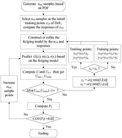
Figure 1.
Flowchart of SPAK method.
Step 1. Initialization. Generate a population of sample points set based on PDF in the design space. It presents the candidate training points of the active learning process. The population of will be changed greater if the condition of updating is satisfied.
Step 2. Define original DoE. In order to build an initial Kriging surrogate model, a DoE contains samples that are stochastically selected from or the Latin hypercube sampled in the truncated domain as [μx ± 5σx]. Then, the performance function is invoked to calculate the responses of these samples. The size of samples in the original DoE usually is small. In the cited paper [4], the number is larger with the number of random variables increased.
Step 3. Construct or refine the Kriging model. The Kriging model is constructed or refined based on the current DoE and responses of these training points. Here, the toolbox of DACE is recommended.
Step 4. Predict using the Kriging model. Kriging predictions , variances , and correlation coefficient vector for with Equations (6)–(8) are obtained. Then, the probability of failure is obtained based on Equation (1).
Step 5. Identify new training points in semi-parallel. In this step, the two learning functions in Equations (15) and (16) are calculated for all sample points, simultaneously. The new potential training points are identified, where and reach the minimum. For most situations, learning functions are primarily based on predictions and variances , they are the same point for high probability. So it will only add one new point to the current training points. Oppositely, a point with a low correlation to the current training points is most likely different from the point based on the U function. Then, both of the two points will be added to the current training points parallelly.
Step 6. The stopping criterion of the learning process. If the best next points are identified with the learning functions, the values of the corresponding learning functions are compared to the stopping criterion in Equation (18).
Step 7. Update DoE with new points. If the stopping criterion in Step 6 is not satisfied, the learning carries on and the new points are evaluated on the performance function. The learning process turns back to Step 3 to refine the new surrogate model with the updated DoE composed of or points.
Step 8. Compute . If the stopping criterion in Step 6 is achieved, then the learning is finished and the Kriging surrogate model is precise enough. As a result, it remains to be seen if is an appropriate size for the MCS. If the size is too small, the probability of failure is trustless. Here, it is acceptable to have a coefficient of variation below 2%. It is estimated as Equation (19):
Step 9. Update Monte Carlo population. If is too large, the Monte Carlo population will be added, which is generated like in Step 1. Then, SPAK turns to Step 4 to forecast the added new population and the active learning method carries on until the stopping criterion is met again. In order to improve efficiency, the evaluations of previous performance function are continually used.
Step 10. End of SPAK. If is lower than the target, SPAK stops and the last estimation of the failure probability is considered as the result of the performance function.
The new learning function and semi-parallel active learning method based on Kriging are illustrated above, and the learning method can be programed in Matlab 2016b by MathWorks Inc, Natick, MA, USA.
4. Numerical Examples
The performance of a complex system is usually affected by various uncertainties, such as variant loads and material degradation [56]. It is not practicable to directly evaluate the system using brute force MCS because it would take too much time and calculation to study the reliability of a complex system with uncertain factors. Therefore, we usually adopt other more efficient methods. A surrogate model is an effective method to replace complex engineering problems in reliability analysis.
To facilitate comparison with existing methods, in this section, three examples are tested to illustrate the advantage of the SPAK method. These are general examples of reliability analysis from references [5,57,58]. First, a highly nonlinear curve function is tested to observe the process of different methods. Next, the six-hump camel-back (SC) function with two dimensions is evaluated. Low-dimensional examples are easy to display graphically, so they can show the learning processes of training points for each iteration, and reveal the different characteristics of the learning functions. Lastly, a nonlinear and high dimensions analytical function with the dynamic response of a nonlinear oscillator is tested. This example demonstrates the effectiveness of high dimensional nonlinear problems. The failure probabilities of the three examples are also significantly reduced, which increases the difficulty of reliability analysis. Through comparison, it is found that the proposed SPAK has higher efficiency, accuracy, and better practicability. The examples are experimented by Matlab.
4.1. Example 1: Highly Nonlinear Curve Function
The first mathematical example, designed to find the extreme response of , is employed to demonstrate the difference of the new training points among the typical Kriging surrogate model methods. The highly nonlinear performance function with one-dimensional space, cited in paper [57], is provided as Equation (20).
where variable x is within the interval [0, 5]. The global minimum occurs at x = 4.515 with G(4.515) = −2.5036, whereas the local minimum is located at x = 1.957 with G(1.957) = 3.9824, shown in Figure 2.
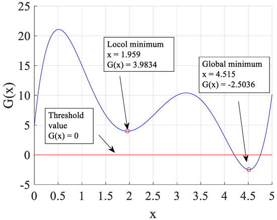
Figure 2.
Performance function of mathematical example.
The performance function is firstly evaluated at initial samples : [0, 1, 2, 2.5, 5], and the obtained performance function values are : [5, 15, 4.004, 6.630, 10.148]. With these initial sample points, the one-dimensional surrogate model can be built to approximate the limit state function . In order to clarify the difference of the modeling process among the methods, the random Kriging method without the learning process is built by 15 points. Based on the learning functions and stopping criterions of different methods, the learning processes are shown as Table 1 and Figure 3. The EGO achieves convergence in nine iterations, the AK and SPAK require 10 and six iterations, respectively. It should be noted that SPAK adds two training points at the first, second and fifth iterations; thus, reduces the number of iterations. So, SPAK is the most efficient.

Table 1.
Results of adding training points for different methods for Example 1.
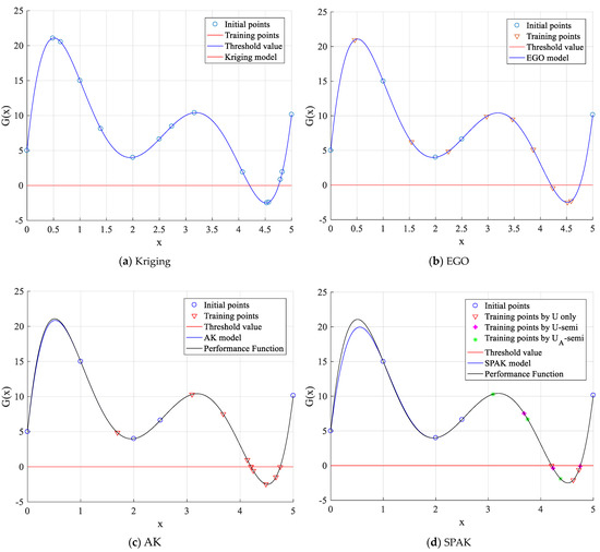
Figure 3.
Training process of surrogate models for Example 1.
In Figure 3, the EGO adds the new points near extreme point with a high probability. It seems more efficient than the AK and SPAK on a global space to identify the extreme value of the performance function. However, for the reliability analysis, under the premise of global modeling, more attention should be paid to the threshold region to determine a critical boundary. Based on the learning function in Equation (15), the AK selects a new point that may be crossed, as shown in Figure 3c. The SPAK considers the correlation between sample points and training points based on Equation (16), the added training points are shown clearly in Figure 3d. Meanwhile, SPAK may add the two new training points in once iterated parallelly; the training points are shown as a plus sign (+) and an asterisk (*) in Figure 3d.
The result of the performance function near the critical region has the most direct effect on the failure probability. Therefore, we choose the extreme point and the vicinity of the critical region as the main area of error analysis. Furthermore, in the interval , the performance function occurs twice out-crossing. For the sake of comparison, the residual error is determined between the actual and predicted values, as described in Equation (21), and the residual errors of several surrogate model approaches are illustrated in Figure 4.
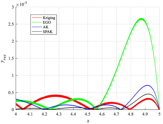
Figure 4.
Residual error of different methods in interval x ∈ [4, 5].
The EGO has the maximum residual error and the standard deviation . The AK follows with and . The Kriging and SPAK are similar. However, when the sample points change, the calculation results of the Kriging method are unstable without a learning process. The SPAK performs even better with and . The surrogate model based on SPAK near the critical region is accurate enough. It is verified that SPAK has a good balance between efficiency and accuracy by semi-parallel learning.
4.2. Example 2: Six-Hump Camel Back Function
The six-hump camel back function is used for the second example [58]. The design space of the SC function in this paper is smaller compared to the original function, as shown in Equation (22). The design variables are uniform distribution in the interval . This function has six minimums, one of which is global minimum, which occurs at with , as indicated by the asterisk in Figure 5. To simulate a small probability of failure, the function is shifted up by one unit.
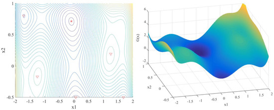
Figure 5.
Contour map and 3D map of SC function.
Fifteen initial training points are generated by uniform random sampling. The surrogate models are constructed and refined by different training methods. The training process is shown in Figure 6. For the random Kriging surrogate model, 60 points are used for random sample training, which is shown in Figure 6a. Due to the randomness, the training points are uncontrollable, and the accuracy near the threshold value of the surrogate model without learning process is not guaranteed. The EGO adds the 20 training points mainly near the area around the two extreme points in Figure 6b, and the other areas of training are disregarded. In interval , the AK and SPAK train the surrogate models around the threshold value, AK adds seven points in Figure 6c, and SPAK adds six points in Figure 6d. It is important to emphasize that SPAK adds the training points semi-parallel, the triangle training points are generated based on the U function in sequential, while the plus training points based on the and the asterisk points based on the U function are in parallel. Therefore, SPAK only iterates 14 times with 26 training points. It has significantly fewer iterations than the AK.
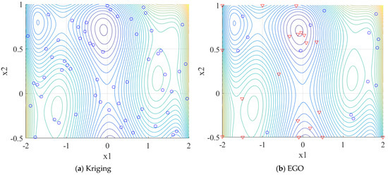
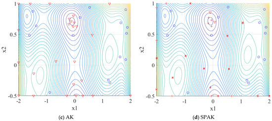
Figure 6.
Training process of once for Example 2 (Ο: initial points, ▽: Sequential training points, * and + are parallel training points).
Furthermore, to eliminate the contingency of the results caused by the initial samples, 20 groups of random samples are selected for the experiment, and the average values of 20 results are finally taken for comparisons. Table 2 shows the results among random Kriging, AK, EGO, SPAK, and brute MCS. The true failure probability is calculated as 0.002971 based on MCS with 1 × 10⁶ sampling evaluations. The results obtained by the four methods are quite different. The random Kriging method has the maximal relative error 11.63%. Obviously, this method is no longer applicable to the problem of small failure probability. The EGO has error 3.036%, better than the random Kriging, and only needs 35.45 number of function evaluations (NoF) and 20.45 NoI. The NoF based on AK and SPAK is close to the former, 38.85, and the latter, 39.1; however, SPAK has fewer NoI than AK, which only has 14.2 iterations. Iteration determines the number of cycles. There is no doubt that SPAK will be more efficient. In terms of accuracy, SPAK is also the best, with a relative error 0.0471%. The absolute error and of SPAK around the threshold value is reduced, which makes SPAK more accurate. The surrogate model is closer to the real performance function.
Table 2.
Results of different methods for Example 2.
4.3. Example 3: Stochastic Linear Oscillation System
The third example, which is a rare failure probability, deals with a stochastic oscillation system [5]. It consists of a nonlinear undamped single degree of freedom (SDoF) system in Figure 7. The performance function is defined as:
where , and input random vector is given as . The probabilistic characteristics are summarized in Table 3.
Figure 7.
Illustration of the SDoF oscillator system.
Table 3.
Random variables of the SDoF oscillation system.
The results of the example depending on different methods are summarized in Table 4. The MCS method is used to calculate the failure probability with 7 × 10⁶ evaluations. The result based on EGO is inaccurate, with relative errors of 10.42%, though only requires 24.3 evaluations and 9.3 iterations. The SPAK is able to obtain precise results of the rare failure probability, with relative errors that are only 0.154%, far lower than other methods. The SPAK, adding the training points in semi-parallel with the fewer NoF and NoI than AK, is efficient for the reliability analysis of the SDoF oscillation system. It also shows that the increase of random variables has little influence on the project.
Table 4.
Results of different methods for Example 3.
Through the above three examples, it is verified that the proposed method has more efficiency and accuracy than the comparison method for nonlinear and high-dimensional reliability analysis problems. It also indicates that the method will have a wide application value.
5. Application
In addition to general numerical examples, the effectiveness of the proposed method can be verified by practical engineering problems. One aquarium is going to be built in the second basement floor of a commercial building. The acrylic board, which is mostly made of polymethyl methacrylate (PMMA), is used to build the aquarium. To ensure safety in case of fire, according to the national standard Code for Design of Building Fire Protection (GB 50016-2014), it is necessary to conduct a safety and reliability analysis. When PMMA receives heat from the flame, the surface temperature of the board will rise. The board loses its mechanical properties and even combusts, thus, collapses, as shown in Figure 8.
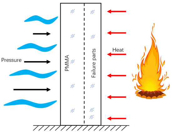
Figure 8.
Aquarium heating model.
The effective thickness model of the board under a different radiation intensity was obtained by the cone calorimeter experiment under 2 h as shown in Figure 9. The expression is shown as Equation (24). The combustion performance and fire resistance that limit the time of building components with various fire resistance grades are specified in national standard GB 50016-2014.
where, b0 is the initial thickness of the board. It equals to 200 mm. q is the radiation intensity of flame, and has a mean value of 40 kW/m2; the variable coefficient is 0.15. The other random variables include depth of water, dimensions of aquarium structure, and material properties of acrylic, which are truncated random variables with μ ± 2σ and they are shown in Figure 10 and Table 5.
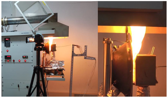
Figure 9.
Cone calorimeter experiment.
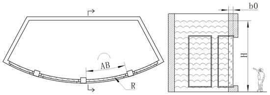
Figure 10.
Aquarium structure and variables.
Table 5.
Random variables of the aquarium.
By establishing a finite element simulation model based on Ansys, the maximum stress with different conditions is calculated. Ansys carries out a finite element simulation and returns the calculation results to Matlab to build and update the surrogate model based on SPAK. The similar finite element simulation and software call method are also used in reference [59]. Figure 11 shows the finite element model of the aquarium and the stress distribution of the result at one point of input variables. The performance function can be simplified as Equation (25), when , it is safe, otherwise, it is unsafe.
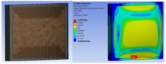
Figure 11.
Finite element model of the aquarium and the stress distribution of the result.
Through DoE and the active learning process, the stress prediction model is constructed and the stress values under the fluctuation of design variables are predicted. Then, the failure probability is calculated by Equations (1) and (25). Because of time constraints, the brute MCS method is not available. Table 6 shows the results of the comparison between Kriging, EGO, AK, and SPAK, without brute MCS. Therefore, the true failure probability cannot be obtained by MCS. The feasible solution is to analyze accuracy by comparing the results among these methods. The result shows that the proposed method is more available for reliability analysis. Firstly, the failure probability based on the proposed SPAK is 5.453 × 10⁻⁵, which is close to AK-MCS and Kriging. It indicates the correctness of SPAK. EGO with a large error is no more applicable. Secondly, the NoF and NoI of SPAK are reduced to 53 and 27; they are both smaller than other methods. The evaluation efficiency is increased by at least 14.5% and iteration efficiency is increased by 35.7%. Based on these two observations, the effectiveness of the proposed method is finally testified.
Table 6.
Results of different methods of the aquarium.
6. Conclusions
Currently, the reliability analysis system is becoming more complex, and the efficiency and accuracy of reliability analysis are also increasing. This paper presents a new algorithm called SPAK that uses Kriging models for small failure probabilities. There are two innovations:
- (1)
- The method proposes a novel learning function that considers the relationship between the training points and samples. It is called the function. Additionally, it is more advanced than the U function, and while it is based on the U function, it is also different from it. The learning function pays attention to the correlation function, predictions and variance, so it overcomes the shortcoming that the training points are always around the area near the threshold. Based on the function, the other essential areas have been highlighted as supplementary. Therefore, the accuracy of the surrogate model based on SPAK is improved.
- (2)
- To enhance the efficiency of iteration, the method proposes the semi-parallel learning process. It will add one or two training points intelligently, which is only based on one stopping criterion. This learning process reduces the number of iterations and enhances efficiency.
The new learning function and intelligent semi-parallel added points are the most significant advantages compared to other parallel learning methods and sequential learning methods.
To test this new method, three numerical examples and a nonlinear and a multidimensional application are studied. We obtain the following results:
- (1)
- The failure probability based on SPAK is more accurate than the Kriging, AK and EGO methods in Example 1 to 3. Especially for Examples 2 and 3, the relative error of the failure probability based on SPAK is only one tenth of the other methods. It verifies the accuracy of this method for the failure probability analysis of the engineering application because the real value of failure probability cannot be obtained for practical engineering problems.
- (2)
- Due to the semi-parallel learning mechanism, the number of iterations required to construct the surrogate model is significantly reduced. In the application of the reliability analysis of the aquarium, evaluation efficiency is increased by at least 14.5% and the iteration efficiency increased by 35.7%. It shows that the semi-parallel learning method has more advantages in computational efficiency, especially in iterative computation.
- (3)
- Due to SPAK being an approximate model construction method, it focuses on the analysis of the accuracy around the model threshold (). Therefore, this method is more suitable for dealing with critical value problems, such as reliability analysis, but may not be the most suitable for solving extreme value problems.
Based on this work, it can be concluded that the proposed algorithm is valuable for constructing reliability the surrogate model. Further, we can combine IS sampling, subset and other methods with SPAK to improve its application value for more rare failure probability analyses. This research group will also carry out relevant research in the follow-up work.
Author Contributions
Conceptualization, C.L. and J.G.; Methodology, Z.L. and X.L.; Formal analysis, Z.L.; Investigation, Y.Q.; Resources, X.L. and Y.Q.; Writing—original draft, Z.L.; Writing—review & editing, J.G.; Funding acquisition, C.L. All authors have read and agreed to the published version of the manuscript.
Funding
This research is supported by the National Natural Science Foundation of China (51905515), and Eyas Program Incubation Project of Zhejiang Provincial Administration for Market Regulation (CY2022221).
Institutional Review Board Statement
Not applicable.
Informed Consent Statement
Not applicable.
Data Availability Statement
Not applicable.
Conflicts of Interest
The authors declare no conflict of interest.
References
- Younès, A.; Emmanuel, P.; Didier, L.; Leila, K. Reliability-based design optimization applied to structures submitted to random fatigue loads. Struct. Multidiscip. Optim. 2017, 55, 1471–1482. [Google Scholar]
- Xie, S.; Pan, B.; Du, X. High dimensional model representation for hybrid reliability analysis with dependent interval variables constrained within ellipsoids. Struct. Multidiscip. Optim. 2017, 56, 1493–1505. [Google Scholar] [CrossRef]
- Kassem, M.; Hu, Z.; Zissimos, P.M.; Igor, B.; Monica, M. System reliability analysis using component-level and system-level accelerated life testing. Reliab. Eng. Syst. Saf. 2021, 214, 107755. [Google Scholar]
- Echard, B.; Gayton, N.; Lemaire, M. AK-MCS: An active learning reliability method combining Kriging and Monte Carlo Simulation. Struct. Saf. 2011, 33, 145–154. [Google Scholar] [CrossRef]
- Zhang, X.; Wang, L.; Sørensen, J.D. REIF: A novel active-learning function toward adaptive Kriging surrogate models for structural reliability analysis. Reliab. Eng. Syst. Saf. 2019, 185, 440–454. [Google Scholar] [CrossRef]
- Hu, Z.; Du, X. Reliability analysis for hydrokinetic turbine blades. Renew. Energy 2012, 48, 251–262. [Google Scholar] [CrossRef]
- Jiang, C.; Wang, D.; Qiu, H.; Gao, L.; Chen, L.; Yang, Z. An active failure-pursuing Kriging modeling method for time-dependent reliability analysis. Mech. Syst. Signal Process. 2019, 129, 112–129. [Google Scholar] [CrossRef]
- Zhang, J.; Taflanidis, A. Bayesian model averaging for Kriging regression structure selection. Probabilistic Eng. Mech. 2019, 56, 58–70. [Google Scholar] [CrossRef]
- Yin, J.; Du, X. Active learning with generalized sliced inverse regression for high-dimensional reliability analysis. Struct. Saf. 2022, 94, 102151. [Google Scholar] [CrossRef]
- Tran, N.-T.; Do, D.-P.; Hoxha, D.; Vu, M.-N.; Armand, G. Kriging-based reliability analysis of the long-term stability of a deep drift constructed in the Callovo-Oxfordian claystone. J. Rock Mech. Geotech. Eng. 2021, 13, 1033–1046. [Google Scholar] [CrossRef]
- Zhou, C.; Li, C.; Zhang, H.; Zhao, H.; Zhou, C. Reliability and sensitivity analysis of composite structures by an adaptive Kriging based approach. Compos. Struct. 2021, 278, 114682. [Google Scholar] [CrossRef]
- Ling, C.; Lu, Z.; Zhu, X. Efficient methods by active learning Kriging coupled with variance reduction based sampling methods for time-dependent failure probability. Reliab. Eng. Syst. Saf. 2019, 188, 23–35. [Google Scholar] [CrossRef]
- Zuev, K.M.; Beck, J.L.; Au, S.-K.; Katafygiotis, L.S. Bayesian post-processor and other enhancements of Subset Simulation for estimating failure probabilities in high dimensions. Comput. Struct. 2012, 92–93, 283–296. [Google Scholar] [CrossRef]
- Liu, Y.; Li, L.; Zhao, S.; Zhou, C. A reliability analysis method based on adaptive Kriging and partial least squares. Probabilistic Eng. Mech. 2022, 70, 103342. [Google Scholar] [CrossRef]
- Zhang, X.; Lu, Z.; Cheng, K. AK-DS: An adaptive Kriging-based directional sampling method for reliability analysis. Mech. Syst. Signal Process. 2021, 156, 107610. [Google Scholar] [CrossRef]
- Liu, Z.; Zhang, J.; Wang, C.; Tan, C.; Sun, J. Hybrid structural reliability method combining optimized Kriging model and importance sampling. Acta Aeronaut. Astronaut. Sin. 2013, 34, 1347–1355. [Google Scholar]
- Li, S.; Caracogli, L. Surrogate model Monte Carlo simulation for stochastic flutter analysis of wind turbine blades. J. Wind. Eng. Ind. Aerodyn. 2019, 188, 43–60. [Google Scholar] [CrossRef]
- Zhu, Z.; Du, X. Reliability Analysis with Monte Carlo Simulation and Dependent Kriging Predictions. J. Mech. Des. 2016, 138, 121403. [Google Scholar] [CrossRef]
- Nannapaneni, S.; Hu, Z.; Mahadevan, S. Uncertainty quantification in reliability estimation with limit state surrogates. Struct. Multidiscip. Optim. 2016, 54, 1509–1526. [Google Scholar] [CrossRef]
- Li, X.; Gong, C.; Gu, L.; Gao, W.; Jing, Z.; Su, H. A sequential surrogate method for reliability analysis based on radial basis function. Struct. Saf. 2018, 73, 42–53. [Google Scholar] [CrossRef]
- Navid, V.; Srinivas, S.; Ana, I. Response surface based reliability analysis of critical lateral buckling force of subsea pipelines. Mar. Struct. 2022, 84, 103246. [Google Scholar]
- Jahanbakhshi, A.; Nadooshan, A.A.; Bayareh, M. Multi-objective optimization of microchannel heatsink with wavy microtube by combining response surface method and genetic algorithm. Eng. Anal. Bound. Elements 2022, 140, 12–31. [Google Scholar] [CrossRef]
- Thakre, U.; Mote, R.G. Uncertainty quantification and statistical modeling of selective laser sintering process using polynomial chaos based response surface method. J. Manuf. Process. 2022, 81, 893–906. [Google Scholar] [CrossRef]
- Biswarup, B. Structural reliability analysis by a Bayesian sparse polynomial chaos expansion. Struct. Saf. 2021, 90, 102074. [Google Scholar]
- Yang, T.; Zou, J.-F.; Pan, Q. A sequential sparse polynomial chaos expansion using Voronoi exploration and local linear approximation exploitation for slope reliability analysis. Comput. Geotech. 2021, 133, 104059. [Google Scholar] [CrossRef]
- Aghatise, O.; Faisal, K.; Salim, A. An active learning polynomial chaos Kriging metamodel for reliability assessment of marine structures. Ocean. Eng. 2021, 235, 109399. [Google Scholar]
- Feng, J.; Liu, L.; Wu, D.; Li, G.; Beer, M.; Gao, W. Dynamic reliability analysis using the extended support vector regression (X-SVR). Mech. Syst. Signal Process. 2019, 126, 368–391. [Google Scholar] [CrossRef]
- Atin, R.; Subrata, C. Reliability analysis of structures by a three-stage sequential sampling based adaptive support vector regression model. Reliab. Eng. Syst. Saf. 2022, 219, 108260. [Google Scholar]
- Wang, J.; Li, C.; Xu, G.; Li, Y.; Kareem, A. Efficient structural reliability analysis based on adaptive Bayesian support vector regression. Comput. Methods Appl. Mech. Eng. 2021, 387, 114172. [Google Scholar] [CrossRef]
- Chocat, R.; Beaucaire, P.; Debeugny, L.; Lefebvre, J.-P.; Sainvitu, C.; Breitkopf, P.; Wyart, E. Damage tolerance reliability analysis combining Kriging regression and support vector machine classification. Eng. Fract. Mech. 2019, 216, 106514. [Google Scholar] [CrossRef]
- Ling, C.; Lu, Z.; Feng, K. An efficient method combining adaptive Kriging and fuzzy simulation for estimating failure credibility. Aerosp. Sci. Technol. 2019, 92, 620–634. [Google Scholar] [CrossRef]
- Arcidiacono, G.; Berni, R.; Cantone, L.; Nikiforova, N.; Placidoli, P. A Kriging modeling approach applied to the railways case. Procedia Struct. Integr. 2018, 8, 163–167. [Google Scholar] [CrossRef]
- Giovanni, V.; Ernesto, B.; Łukasz, Ł. A Kriging-assisted multiobjective evolutionary algorithm. Appl. Soft Comput. 2017, 58, 155–175. [Google Scholar]
- Ma, Y.-Z.; Liu, M.; Nan, H.; Li, H.-S.; Zhao, Z.-Z. A novel hybrid adaptive scheme for Kriging-based reliability estimation—A comparative study. Appl. Math. Model. 2022, 108, 1–26. [Google Scholar] [CrossRef]
- Mishra, B.; Kumar, A.; Zaburko, J.; Sadowska-Buraczewska, B.; Barnat-Hunek, D. Dynamic Response of Angle Ply Laminates with Uncertainties Using MARS, ANN-PSO, GPR and ANFIS. Materials 2021, 14, 395. [Google Scholar] [CrossRef] [PubMed]
- Zhang, C.; Shafieezadeh, A. Simulation-free reliability analysis with active learning and Physics-Informed Neural Network. Reliab. Eng. Syst. Saf. 2022, 226, 108716. [Google Scholar] [CrossRef]
- Sepahvand, K.; Marburg, S.; Hardtke, H.-J. Stochastic structural modal analysis involving uncertain parameters using generalized polynomial chaos expansion. Int. J. Appl. Mech. 2011, 3, 587–606. [Google Scholar] [CrossRef]
- Fauriat, W.; Gayton, N. AK-SYS: An adaptation of the AK-MCS method for system reliability. Reliab. Eng. Syst. Saf. 2014, 123, 137–144. [Google Scholar] [CrossRef]
- Echard, B.; Gayton, N.; Lemaire, M.; Relun, N. A combined Importance Sampling and Kriging reliability method for small failure probabilities with time-demanding numerical models. Reliab. Eng. Syst. Saf. 2013, 111, 232–240. [Google Scholar] [CrossRef]
- Xiao, S.; Oladyshkin, S.; Nowak, W. Reliability analysis with stratified importance sampling based on adaptive Kriging. Reliab. Eng. Syst. Saf. 2020, 197, 106852. [Google Scholar] [CrossRef]
- Huang, S.-Y.; Shao-He, Z.; Liu, L.-L. A new active learning Kriging metamodel for structural system reliability analysis with multiple failure modes. Reliab. Eng. Syst. Saf. 2022, 228, 108761. [Google Scholar] [CrossRef]
- Zhu, L.; Qiu, J.; Chen, M.; Jia, M. Approach for the structural reliability analysis by the modified sensitivity model based on response surface function-Kriging model. Heliyon 2022, 8, e10046. [Google Scholar] [CrossRef] [PubMed]
- Hao, P.; Feng, S.; Liu, H.; Wang, Y.; Wang, B.; Wang, B. A novel Nested Stochastic Kriging model for response noise quantification and reliability analysis. Comput. Methods Appl. Mech. Eng. 2021, 384, 113941. [Google Scholar] [CrossRef]
- Wang, D.; Qiu, H.; Gao, L.; Jiang, C. A single-loop Kriging coupled with subset simulation for time-dependent reliability analysis. Reliab. Eng. Syst. Saf. 2021, 216, 107931. [Google Scholar] [CrossRef]
- Zuhal, L.R.; Faza, G.A.; Palar, P.S.; Liem, R.P. On dimensionality reduction via partial least squares for Kriging-based reliability analysis with active learning. Reliab. Eng. Syst. Saf. 2021, 215, 107848. [Google Scholar] [CrossRef]
- Li, X.; Zhu, H.; Chen, Z.; Ming, W.; Cao, Y.; He, W.; Ma, J. Limit state Kriging modeling for reliability-based design optimization through classification uncertainty quantification. Reliab. Eng. Syst. Saf. 2022, 224, 108539. [Google Scholar] [CrossRef]
- Jones, D.R.; Schonlau, M.; Welch, W.J. Efficient Global Optimization of Expensive Black-Box Functions. J. Glob. Optim. 1998, 13, 455–492. [Google Scholar] [CrossRef]
- Bichon, B.J.; Eldred, M.S.; Swiler, L.P.; Mahadevan, S.; McFarland, J.M. Efficient Global Reliability Analysis for Nonlinear Implicit Performance Functions. AIAA J. 2008, 46, 2459–2468. [Google Scholar] [CrossRef]
- Bichon, B.; Eldred, M.; Swiler, L.; Mahadevan, S.; McFarland, J. Multimodal Reliability Assessment for Complex Engineering Applications using Efficient Global Optimization. In Proceedings of the 48th AIAA/ASME/ASCE/AHS/ASC Structures, Structural Dynamics, and Materials Conference, Honolulu, HI, USA, 23–26 April 2007. [Google Scholar] [CrossRef]
- Zhang, J.; Xiao, M.; Gao, L. An active learning reliability method combining Kriging constructed with exploration and exploitation of failure region and subset simulation. Reliab. Eng. Syst. Saf. 2019, 188, 90–102. [Google Scholar] [CrossRef]
- Lv, Z.; Lu, Z.; Wang, P. A new learning function for Kriging and its applications to solve reliability problems in engineering. Comput. Math. Appl. 2015, 70, 1182–1197. [Google Scholar] [CrossRef]
- Sun, Z.; Wang, J.; Li, R.; Tong, C. LIF: A new Kriging based learning function and its application to structural reliability analysis. Reliab. Eng. Syst. Saf. 2017, 157, 152–165. [Google Scholar] [CrossRef]
- Krige, D.G. A statistical approach to some basic mine valuation problems on the Witwatersrand. J. Chem. Metall. Min. Eng. Soc. S. Afr. 1951, 52, 119–139. [Google Scholar]
- Ranjan, P.; Bingham, D.; Michailidis, G. Sequential Experiment Design for Contour Estimation from Complex Computer Codes. Technometrics 2008, 50, 527–541. [Google Scholar] [CrossRef]
- Chen, W.; Xu, C.; Shi, Y.; Ma, J.; Lu, S. A hybrid Kriging-based reliability method for small failure probabilities. Reliab. Eng. Syst. Saf. 2019, 189, 31–41. [Google Scholar] [CrossRef]
- Qian, H.-M.; Huang, H.-Z.; Li, Y.-F. A novel single-loop procedure for time-variant reliability analysis based on Kriging model. Appl. Math. Model. 2019, 75, 735–748. [Google Scholar] [CrossRef]
- Wang, Z.; Wang, P. A Nested Extreme Response Surface Approach for Time-Dependent Reliability-Based Design Optimization. J. Mech. Des. 2012, 134, 121007. [Google Scholar] [CrossRef]
- Gao, Y.; Wang, X. A sequential optimization method with multi-point sampling criterion based on Kriging surrogate model. Eng. Mech. 2012, 29, 90–95. [Google Scholar] [CrossRef]
- Mishra, B.B.; Kumar, A.; Samui, P.; Roshni, T. Buckling of laminated composite skew plate using FEM and machine learning methods. Eng. Comput. 2020, 38, 501–528. [Google Scholar] [CrossRef]
Disclaimer/Publisher’s Note: The statements, opinions and data contained in all publications are solely those of the individual author(s) and contributor(s) and not of MDPI and/or the editor(s). MDPI and/or the editor(s) disclaim responsibility for any injury to people or property resulting from any ideas, methods, instructions or products referred to in the content. |
© 2023 by the authors. Licensee MDPI, Basel, Switzerland. This article is an open access article distributed under the terms and conditions of the Creative Commons Attribution (CC BY) license (https://creativecommons.org/licenses/by/4.0/).