Comparison and Improvement of 3D-Multilateration for Solving Simultaneous Localization of Drones and UWB Anchors

Abstract

Drone fleets have attracted a lot of attention from the research community in recent years. One of the biggest challenges in deploying such systems is localization. While GNSS localization systems can only be effective in open outdoor environments, new solutions based on radio sensors (e.g., ultra-wideband) are increasingly being used for localization in various situations and environments. However, self-localization without prior knowledge of anchor positions remains an open problem, which, for example, makes it impossible to track a moving target. In this article, we provide a comparison of different variants of gradient descent-based algorithms, with a new improved variant, for solving the localization problem using relative distance measurements and multilateration. Extensive simulation results are provided, varying the number of neighboring nodes for multilateration, algorithm initialization, and cost functions, in addition to accounting for node positioning errors and ultra-wideband sensor noise. They help set the adequate rate for fixed step descent when used and produce a damping effect in the variable step rate, which will otherwise diverge. In particular, we consider three scenarios: (i) self-localization of anchors; (ii) tracking moving targets using ultra-wideband range sensors; and (iii) simultaneously estimating unknown positions of ultra-wideband anchors and mobile agents (drones). The latter shows a great improvement in localization accuracy.

1. Introduction and Related Work

In recent years, drones have aroused the interest of the scientific community as they offer huge potential in many civil applications [1,2], such as first aid in natural disasters or inspection to prevent forest fires [3,4,5]. With the evolution of technology, the miniaturization of electronics, and the increase in the processing power of on-board systems, it is currently possible to carry out complex missions with small and inexpensive drones, or even fleets of drones [6,7]. Drone fleet missions have proven to be more efficient in terms of scalability, survivability, and rapid response. However, swarm flight poses several research problems. The most important is undoubtedly the localization of drones in a global or relative reference system. Depending on the type of environment (indoor, outdoor, industrial [8], etc.), but also on the type of system to be localized, there are different levels of localization complexity [9].

GNSS (Global Navigation Satellite System) positioning, such as GPS, is the most commonly used solution for outdoor localization [10]. However, the localization accuracy may be insufficient, especially for missions operated in swarms, or simply ineffective in indoor environments. To overcome this limitation, other localization systems can be used such as cameras [11] and inertial measurement systems [12]. Some promising methods use RF chips implementing different standards such as RFID, Bluetooth [13], or WiFi [14,15]. Since these methods are low-cost, require low processing power, and have a long range [16], this article will focus on RF-based methods. The best known RF technique is the Received Signal Strength Indicator (RSSI) [17,18,19,20]. Knowing the power emitted and the propagation attenuation model makes it possible to calculate the propagation distance. With the use of specific antennas, it is possible to obtain the Angle of Arrival (AOA) of the transmitted wave and to obtain the position by triangulation. Using the propagation speed, travel time measurement techniques such as Time of Arrival (ToA) or Time Difference of Arrival (TDoA) [21,22,23,24] allows one to obtain the position with a trilateration calculation. In particular, TDoA-based ultra-wideband (UWB) sensors are very popular [25,26] as they allow very accurate distance measurements at a relatively low cost.

RF-based positioning can be solved analytically [27,28,29,30] when exact models are known or using numerical optimization methods. Several optimization algorithms can be found in the literature [31] to solve multilateration. It should be mentioned that the computation may be difficult due to the non-linearity and/or non-convexity of the estimation problem, potentially leading to local minima or divergence. An interesting approach [32], based on a variant of the original Space Alternating Generalized Expectation Maximization (SAGE) algorithm [33], leads to the joint estimation of the Direction of Arrival (DoA), time-delay, and range estimation, aiming to improve the estimation accuracy of communicating vehicles.

This work deals with the multilateration localization problem in non-GPS environments, using UWB relative distance measurements whose anchoring positions are unknown or are known but with uncertainties. We address the problem of localization in different scenarios, including (i) the positioning of a fleet of drones based on RF measurements to anchors with poorly known positions; (ii) estimating the position of UWB anchors based on the distances measured to one or more drones located by on-board sensors; and (iii) simultaneously combining the two estimates of the positions of the anchors and the drones to improve the localization accuracy of the system as a whole. The estimation problem is solved using gradient-descent-based optimization while considering different formulations for the cost functions and proposing a new adaptation.

The rest of the paper is organized as follows. Section 2 presents a unified formulation of the estimation problem we address. To solve this problem, different formulations of the gradient descent-based optimization are presented in Section 3. Then, in Section 4, simulation results are described and analyzed before concluding this work in Section 5.

2. Problem Statement

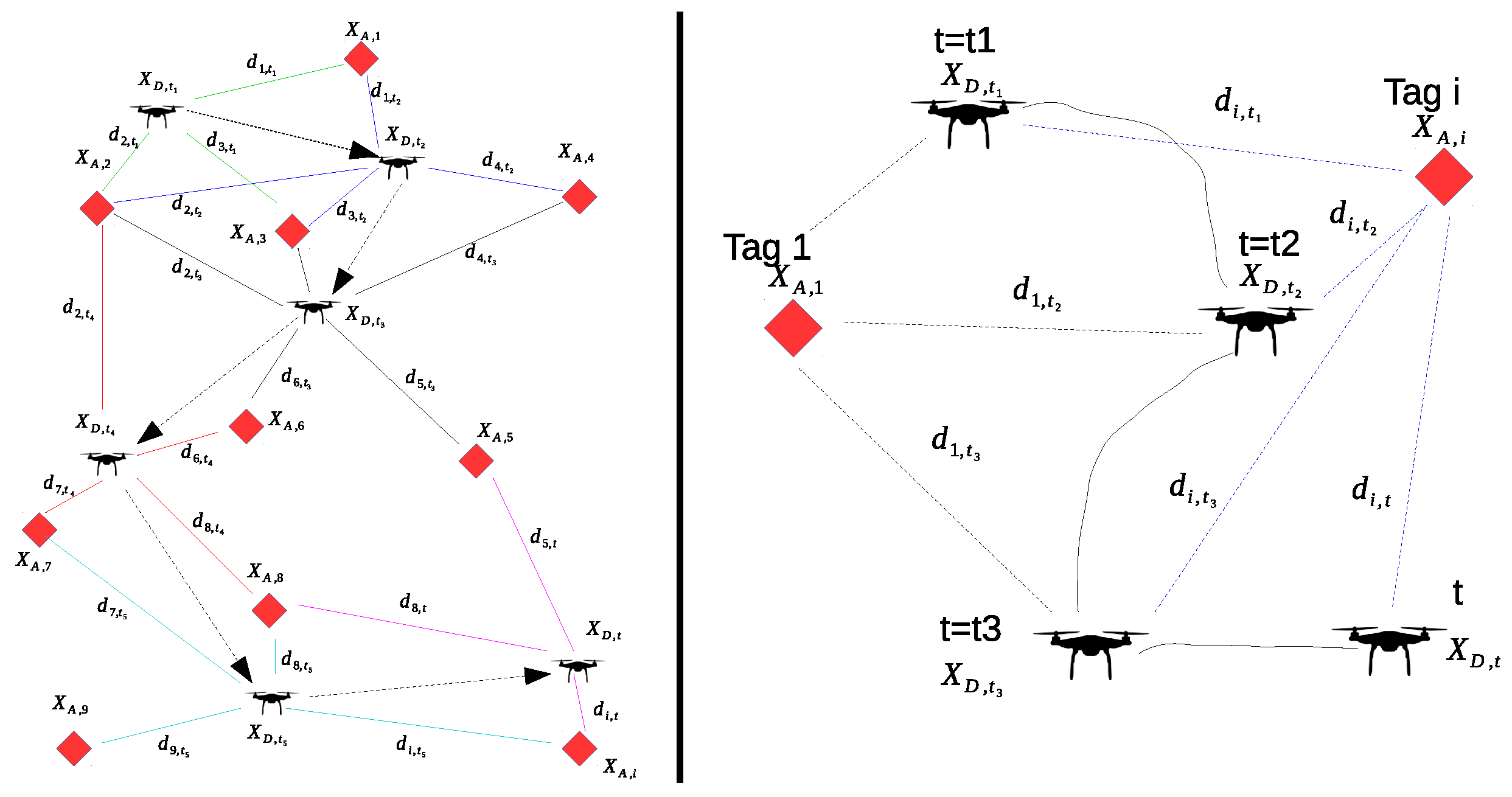
Trilateration, and more generally, multilateration, is an important technique for 3D position estimation using distance measurements to four or more anchors with known position coordinates. Multilateration localization is used here to co-estimate the 3D positions of a set of fixed nodes and mobile agents (drones) capable of taking relative distance measurements in various scenarios. The first scenario consists in retrieving unknown 3D positions of a set of mobile agents given their relative distance measurements to a set of known anchors (Figure 1a). The second scenario (Figure 1b) consists of retrieving the 3D positions of a set of anchors using a set of mobile agents. In this case, an estimate of the positions of the mobile agents is assumed to be given using on-board sensors. The third scenario is a hybrid case where recovered positions of the anchors will improve the localization of moving agents. It deals with the problem of simultaneously obtaining an accurate estimation of the positions of drones and the active fixed sensors.

This work gives a unified formulation to these scenarios, and solves the multilateration estimation problem with and without taking into account noisy range measurements and location uncertainties.

In the following, each agent or active sensor node i of unknown position will be referred to as ${\mathbf{x}}_i={(x_i,y_i,z_i)}^T$, denoting its 3D coordinates in a global reference frame and having $d_{i,j}$ distance measurements to $k\ge 4$ neighboring nodes with known position coordinates, denoted as ${\mathbf{x}}_{\mathbf{n}}j={(x_j,y_j,z_j)}^T,1\le j\le k$.

Position/distance constraints can be formulated by (1) expressing that any node i of unknown an 3D position, ${\mathbf{x}}_i={(x_i,y_i,z_i)}^T$, lies at the intersection of $k\ge 4$ circles centered on the detected neighboring nodes with known positions and having the estimated range $d_{i,j}$ as their radii:

$$\left(\begin{array}{c}{(x_i-x_1)}^2+{(y_i-y_1)}^2+{(z_i-z_1)}^2\\ {(x_i-x_2)}^2+{(y_i-y_2)}^2+{(z_i-z_2)}^2\\ ⋮\\ {(x_i-x_k)}^2+{(y_i-y_k)}^2+{(z_i-z_k)}^2\end{array}\right)=\left(\begin{array}{c}{d}_{i,1}^2\\ d_{i,2}^2\\ ⋮\\ d_{i,k}^2\end{array}\right)$$

(1)

This leads to a nonlinear least squares problem that can have multiple local minima. The authors [34] have proposed a solution to the convex relaxation of this problem, but there will still be no guarantee that the solution will be optimal. Another way to solve this problem is to consider a linear solver by forming differences between pairs of these equations leading to the deletion of quadratic terms in (1). For instance, by subtracting the last component $\left|\right|{\mathbf{x}}_i-{\mathbf{x}}_k{\left|\right|}^2$ from all others in (1), the problem (1) can then be rearranged and reformulated as follows:

$${\mathbf{A}}_{(k-1)\times 3}{\mathbf{x}}_i={\mathbf{D}}_{(k-1)\times 1}$$

(2)

where

$$\mathbf{A}=\left(\begin{array}{ccc}(x_k-x_1)& (y_k-y_1)& (z_k-z_1)\\ (x_k-x_2)& (y_k-y_2)& (z_k-z_2)\\ ⋮\\ (x_k-x_{k-1})& (y_k-y_{k-1})& (z_k-z_{k-1})\end{array}\right); {\displaystyle \mathbf{D}={\displaystyle \frac{1}{2}}\left(\begin{array}{c}{d}_{i,1}^2-d_{i,k}^2+x_k^2-x_1^2+y_k^2-y_1^2+z_k^2-z_1^2\\ d_{i,2}^2-d_{i,k}^2+x_k^2-x_2^2+y_k^2-y_2^2+z_k^2-z_2^2\\ ⋮\\ d_{i,k-1}^2-d_{i,k}^2+x_k^2-x_{k-1}^2+y_k^2-y_{k-1}^2+z_k^2-z_{k-1}^2\end{array}\right)}$$

Note that the matrices $\mathbf{A}$ and $\mathbf{D}$ are expressed only as a function of neighboring nodes whose positions and relative distance measurements are known.

Several methods have been proposed to solve the estimation problem (2). It could be solved using either the least squares approximation or other algebraic methods since, in the general case, the matrix $\mathbf{A}$ is not necessarily square (depending on the number of neighboring nodes with known positions). This provides an exact solution if it exists and an approximate solution otherwise. To be noted, the matrix $\mathbf{A}$ is singular, and the solution does not exist if all the neighboring nodes are collinear. If the measured distances are disturbed by measurement noise, the equalities in (1) and (2) would no longer hold. The problem of finding the unknown positions of the nodes is then approached by forming the residuals of the system and then minimizing a cost function of these residuals. In the following, we study different formulations of the estimation problem with noisy range measurements, harnessing different cost functions to minimize the localization error. They are summarized below in (3)–(6) and will be thoroughly discussed under different conditions in the following sections.

Definition 1 (Problem 1).

The optimal estimate of the unknown position of a node i, ${\mathbf{x}}_i$ having measurements $d_{i,j}$ to nodes ${\mathbf{x}}_{\mathbf{n}}j,j=1\dots k$ with known positions, is usually given by:

$${\mathbf{x}}_i^{🟉}=\underset{{\mathbf{x}}_i\in {\mathbb{R}}^3}{argmin}\sum _{j=1}^k{\left(\parallel {\mathbf{x}}_i-{\mathbf{x}}_{\mathbf{n}}j\parallel -d_{i,j}\right)}^2$$

(3)

This is a nonlinear optimization problem aimed at minimizing the sum of the squares of the residuals between the measured distances and the hypothetical distances based on the known location of nodes.

Definition 2 (Problem 2).

An alternative formulation to the cost function (3) could be defined by the following to provide an optimal node location estimate:

$${\mathbf{x}}_i^{🟉}=\underset{{\mathbf{x}}_i\in {\mathbb{R}}^3}{argmin}\sum _{j=1}^k{\displaystyle \frac{1}{2}}{\left({\parallel {\mathbf{x}}_i-{\mathbf{x}}_{\mathbf{n}}j\parallel }^2-d_{i,j}^2\right)}^2$$

(4)

This still leads to a nonlinear, nonconvex optimization problem, aiming to minimize the quadratic error between the squared measured distances and the squared relative positions of the nodes.

The formulations (3) and (4) do not explicitly take into account uncertainties. However, the nodes of known positions could be affected by uncertainties, and the acquired distances are also affected by measurement errors. In these cases, the previous problems are modified to include position and measurement errors and are formulated as follows:

Definition 3 (Problem 3).

In the presence of positioning and measurement errors, the optimal estimate derived from (3) is given by:

$${\mathbf{x}}_i^{🟉}=\underset{{\mathbf{x}}_i\in {\mathbb{R}}^3}{argmin}\sum _{j=1}^k{\left(\parallel {\mathbf{x}}_i-({\mathbf{x}}_{\mathbf{n}}j+{\mathbf{e}}_{pos})\parallel -(d_{i,j}+e_d)\right)}^2$$

(5)

where${\mathbf{e}}_{pos}$and$e_d$denote the position and range measurement errors, respectively.

Definition 4 (Problem 4).

The alternative formulation derived from (4) of the cost function while including position and measurement errors leads to the optimal estimate:

$${\mathbf{x}}_i^{🟉}=\underset{{\mathbf{x}}_i\in {\mathbb{R}}^3}{argmin}\sum _{j=1}^k{\displaystyle \frac{1}{2}}{\left({\parallel {\mathbf{x}}_i-({\mathbf{x}}_{\mathbf{n}}j+{\mathbf{e}}_{pos})\parallel }^2-{(d_{i,j}+e_d)}^2\right)}^2$$

(6)

Localization by multilateration consists of solving one of the previous formulations of the optimization problems (3)–(6), which differ mainly by the cost functions used and by considering explicitly or not the uncertainties in the position of the anchor nodes and the range measurements. These formulations are of great importance and will impact not only the precision of the solution, but also the computation time and even the possibility of finding a solution to the localization problem.

3. Multilateration Estimation Resolution

Gradient descent (GD) is one of the most used algorithms for many recent applications [35,36] due to its simplicity and computational efficiency in optimizing an objective function. We consider in this work two variants of GD methods to solve multilateration problems (3)–(6) based on fixed or variable rates in the gradient descent step. We also introduce a revisited formulation of the variable step descent. Indeed, it is well known that choosing a proper descent step can be tricky. Too small a descent step leads to slow convergence, while a too large descent step can hinder convergence and cause the utility function to fluctuate around the minimum or even diverge. Some approaches [37] use Line Search methods or variants, solving a second iterative optimization problem under specific conditions to find an appropriate fixed step length.

To solve problems (3)–(6), starting from an initial guess ${\mathbf{x}}_{i,0}\in {\mathbb{R}}^3$ of a node position ${\mathbf{x}}_i$, a sequence of solutions is produced iteratively by:

$${\mathbf{x}}_{i,k+1}={\mathbf{x}}_{i,k}-{\alpha }_k{\mathbf{g}}_k$$

(7)

where ${\mathbf{x}}_{i,k}$ is the position estimate at iteration k, ${\mathbf{g}}_k$ is the gradient of the utility function, and ${\alpha }_k$ is the gradient descent step defined by Equation (8). ${\alpha }_k$ could be constant in a fixed step descent or, depending on H, the Hessian matrix of the utility function. The proposed revisited formulation introduces a damping parameter $0<\beta \le 1$ in the variable step rate:

$${\alpha }_k=\left\{\begin{array}{cc}\alpha \hfill & using the fixed rate step,\hfill \\ {\displaystyle \frac{{\mathbf{g}}_k^T\mathbf{g}}{{\mathbf{g}}_k^{T}H{\mathbf{g}}_k}}\hfill & using the variable rate step,\hfill \\ \beta {\displaystyle \frac{{\mathbf{g}}_k^T\mathbf{g}}{{\mathbf{g}}_k^{T}H{\mathbf{g}}_k}}\hfill & using the revisited formulation.\hfill \end{array}\right.$$

(8)

These methods are implemented and evaluated in the next section, with the objective of finding the optimal parameters and conditions necessary to solve the cases presented by the localization scenarios.

Table 1. Overview of the evaluated methods and the varied parameters in the simulations.

Methods evaluated	GD using a fixed rate step, a variable rate step, and a variable rate step including a damping parameter.
Problem formulation	Cost functions (3)–(6) without and with explicitly including positioning and measurement errors.
Anchor nodes	100 randomly selected sample points in a 3D map.
Algo. initialization	100 randomly chosen initial points.
Number of relative measurements	Varying from 4 to 10 neighboring points and relative distance measurements.

summarizes the different combinations with the evaluated parameters.

4. Simulation Results

To evaluate the resolution methods with respect to the formulations considered, we carry out extended statistical analyses by varying the number of neighboring nodes and the parameters of the algorithms. The simulation environment is a simulated 3D space of 100 m × 100 m × 50 m ($x,y,z$ dimensions, respectively) centered on a global reference frame with the origin $(0,0,0)$. It contains a large population of randomly distributed fixed nodes (anchors) and a set of drones with predefined trajectories. For each test scenario, multilateration localization is solved for 100 randomly selected nodes with unknown positions, using $k\in [4,10]$ randomly selected neighboring nodes of known coordinates and 100 random initial guesses to start the execution of the algorithm. The random character also makes it possible to evaluate the impact of the distribution and the relative positioning of the nodes. They are only constrained to have a minimum relative measurement distance of 1 m. This leads, for each test scenario, to 10,000 simulation tests, run under Matlab on a Linux Ubuntu 16.04 OS with 16 GB of memory and an Intel Core i7-4710MQ processor (using a single 2.5 Ghz core for the simulations).

For the estimation problems (5) and (6) expressing uncertainties, the errors on the assumed known positions of the nodes are modeled by a Gaussian noise centered on the real position of the simulated nodes with a standard deviation ${\sigma }_{{\mathbf{x}}_{\mathbf{n}}}$ determined empirically. Measurement errors are modeled based on the approximation given in (10) [38] and confirmed by our experimental study using UWB sensors in indoor and outdoor environments:

$${\mathbf{e}}_{pos}=\mathcal{N}(0;{\sigma }_{{\mathbf{x}}_{\mathbf{n}}})$$

(9)

$$e_d=e_{uwb}=e_0+e_1{d}_{i,j}+e_2{d}_{i,j}^2+e_3{d}_{i,j}^3$$

(10)

with the following experimentally identified parameters:

$$\begin{array}{cc}{e}_0=2.361e^{-3},\hfill & e_1=1.805e^{-3},\hfill \\ e_2=4.808e^{-5},\hfill & e_3=4.655e^{-7}.\hfill \end{array}$$

4.1. Fixed-Step GD Estimation

Solving a multilateration problem with fixed-step gradient descent can diverge if the step is too large or slow down convergence considerably if it is too small. At the expense of additional optimization cost, some authors [37,39] have proposed to use the backtracking line search algorithm, thus solving an additional optimization problem in order to define a suitable step length that satisfies certain conditions. Here, we propose performing a statistical analysis to determine a good approximation of the best fixed-step descent parameter for each formulation of the estimation problems (3)–(6).

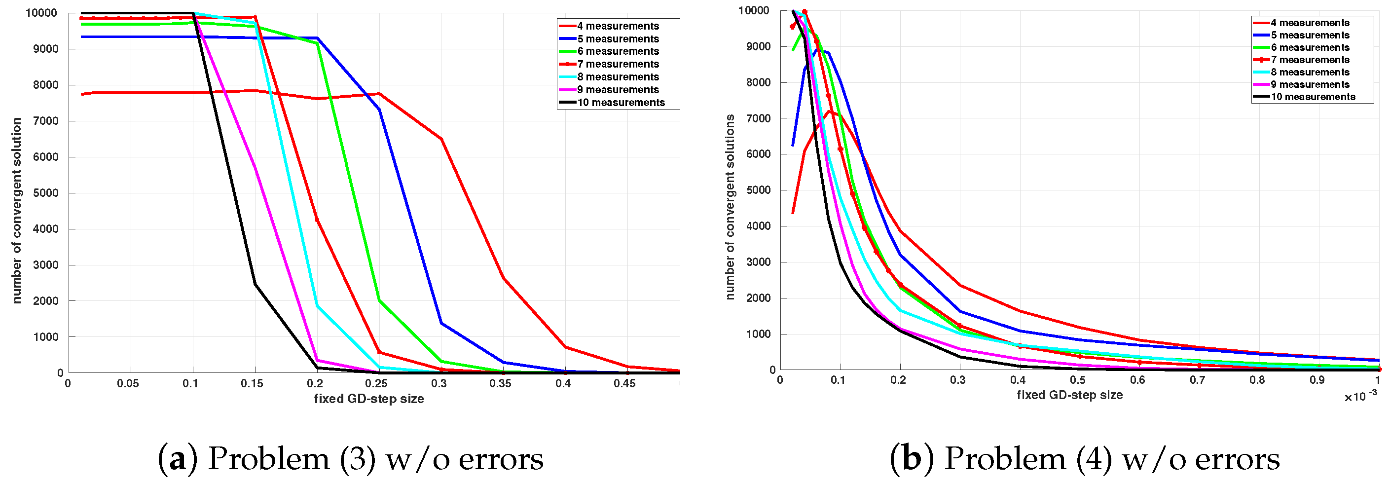
The convergence results for the formulations (3) and (4) (without explicitly considering position and range measurement noises) are presented in Figure 2. A solution is considered convergent if the positioning error, i.e., the Euclidean distance between the real position of the target and its estimate, is less than 20 cm. Obviously, it can be noted that increasing the fixed descent step length reduces the convergence rate, in particular when the number of neighboring nodes used in the estimation increases. Therefore, by reducing the descent step, the convergence rate is increased. Using problem formulation (3), notice the appearance of a plateau whose value depends on the number of neighboring nodes used in multilateration. This means that below a certain value, it is useless to continue to decrease the step of descent, which will lead to increasing the computation time without improving the convergence success. It should be noted that these "plateau" values will be chosen as fixed parameters of the descent step in the comparative simulations. It can also be noted that increasing the number of measurements improves the convergence rates up to a certain threshold (here, 8), beyond which no improvement is detected. 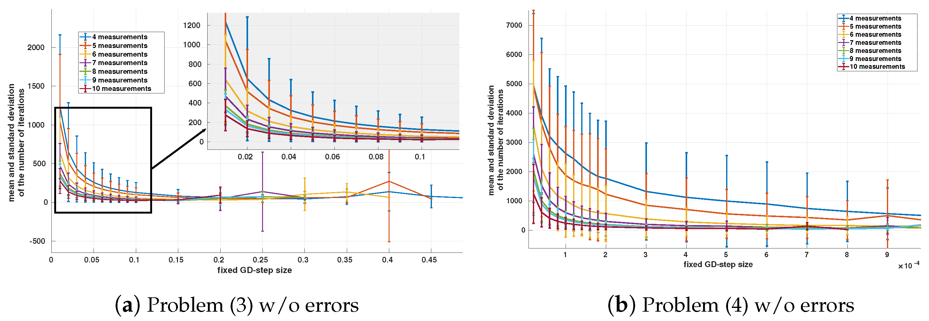Similar observations can be made for the problem formulation (4), noting that convergence for very small step values is extremely slow and the algorithm stops after exceeding the maximum number of iterations. The number of iterations until convergence for both formulations is given in Figure 3 and confirms this observation. It can be concluded that for equivalent performances, problem formulation (4) converges much more slowly than (3).

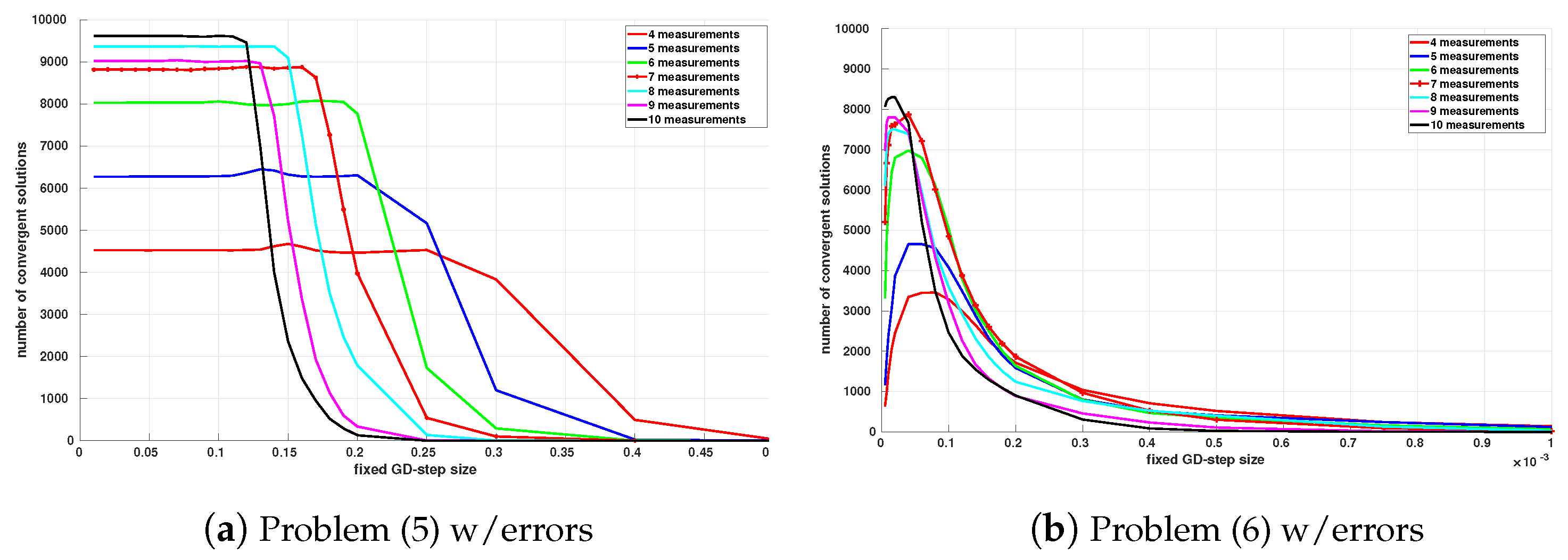
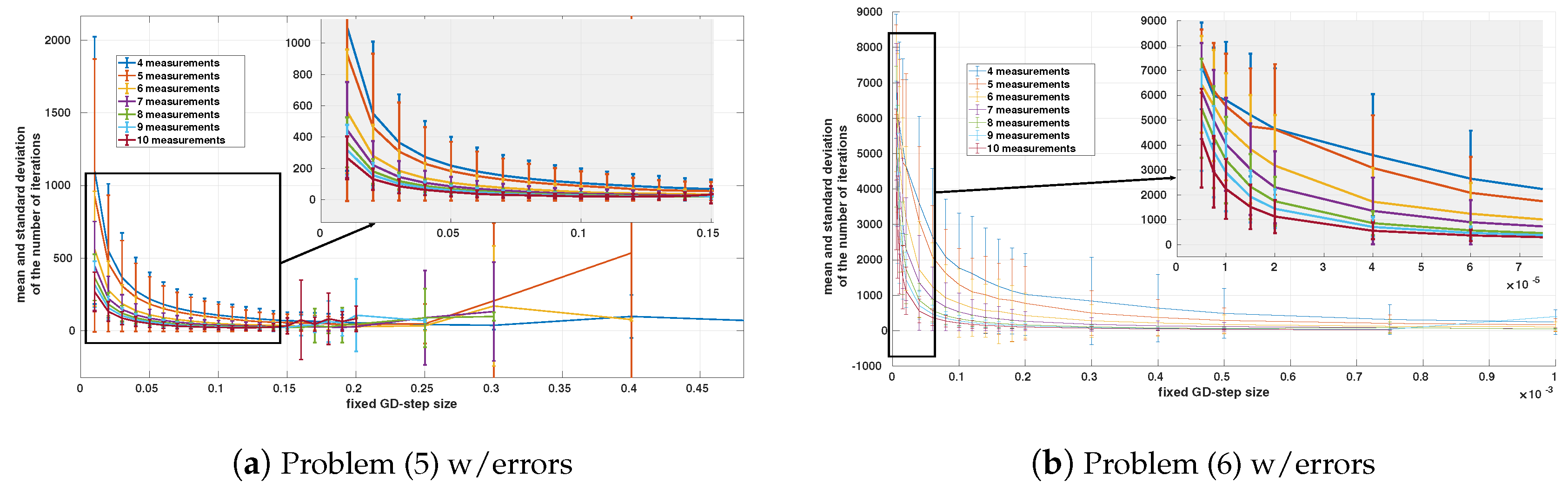
The same tests are carried out by incorporating in the cost functions the position (9) and the measurement (10) error models in the estimation problems (5) and (6). Figure 4 and Figure 5 give the results of convergence and the number of iterations until convergence over 10,000 simulations for the two formulations and for a different number of neighboring nodes, depending the length of the fixed step and the number of distance measurements.

The profiles of the curves are similar to the results of the formulations without error models; the only changes are a decrease in performance due to the integration of errors, which impacts situations with a low number of measurements more significantly. It can also be noticed that the plateau levels are close to the previous values, and at equivalent performance, the numbers of iterations at convergence are lower for the formulation (5) compared to (6).

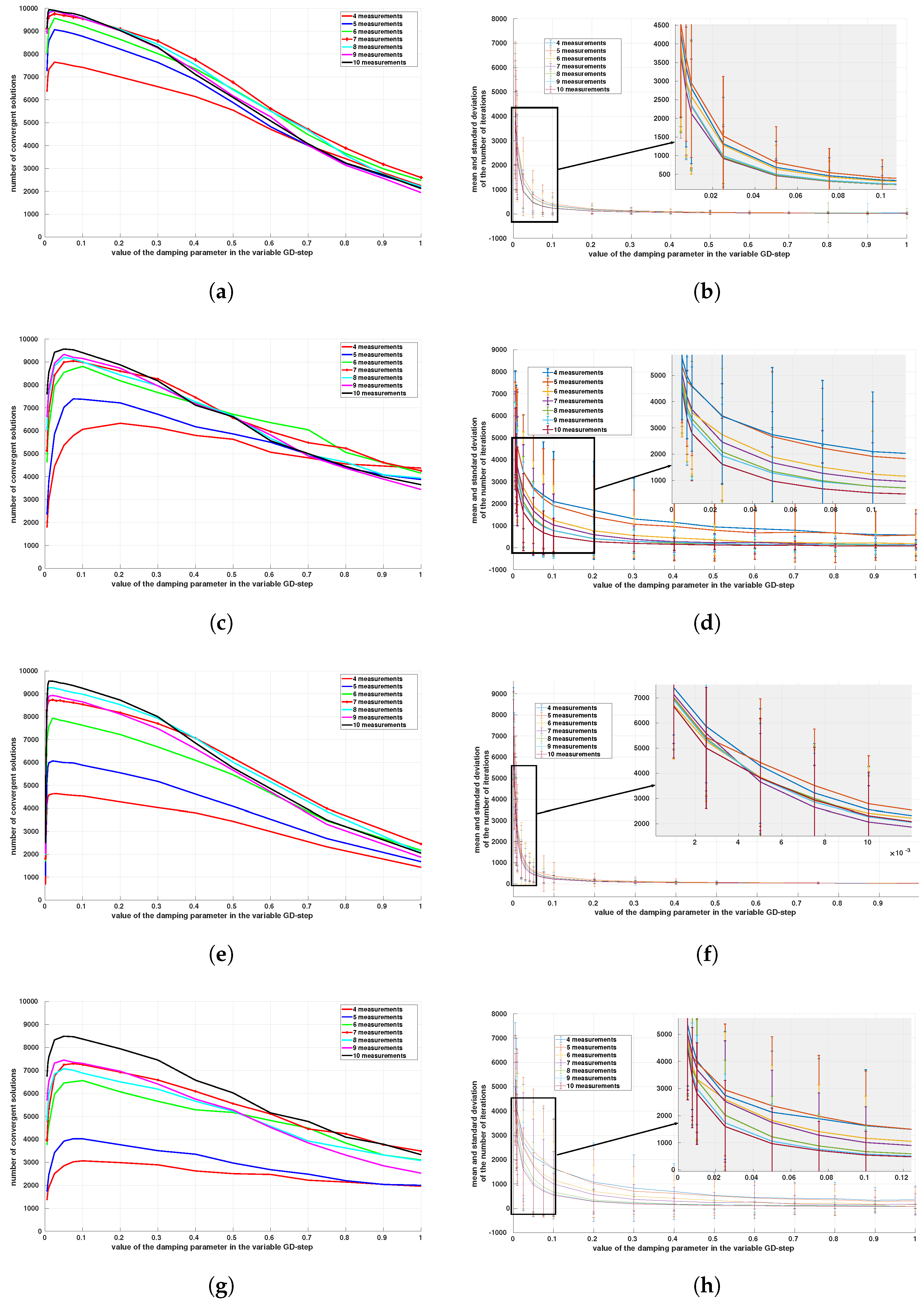
4.2. Variable-Step GD Estimation

An alternative approach to fixed-length step descent is to adapt the rate step to the normalized gradient, as defined by (8). The same scenarios from the previous tests are reconsidered using the variable-step descent algorithm. The simulation results showed a very weak convergence (around 20%) with all the formulations of cost functions, with and without explicit incorporation of error models. This observation motivated us to investigate the problem and led us to reformulate the gradient step by introducing a damping parameter $\beta$, as defined in (8). The results are shown in Figure 6, with and without position and measurement errors. Note that $\beta =1$ corresponds to the classical formulation of the variable-step descent (i.e., without damping).

First, one can notice the increase in convergence rates with the number of relative measurements used in the estimation. This is particularly noticeable for a small number of measurements. Moreover, when the number of measurements exceeds seven, the convergence rate varies very little. Another point to note is the impact of the value of the damping parameter $\beta$. Indeed, using a value close to $0.1$ for the optimization problem (3) gives better results than the classical variable step ($\beta =1$) for any number of measurements.

The analysis of the number of iterations until convergence (second row of Figure 6) shows that reducing the damping parameter improves the convergence results but, consequently, also increases the number of iterations to convergence. For instance, a value $\beta =0.1$ leads to 95% of convergent estimates in less than 500 iterations for optimization problem (3). Similar results are shown for the optimization problem (4) with a slight decrease in performance. It therefore appears more interesting to use the cost function (3) with value $\beta =0.1$ in the case of an adaptive descent with free-error models. While integrating positioning and measurement error models into the formulations, the curves also confirm these trends with a slight drop in performance. This confirms that the cost function (5) seems to give better results than (6), and that a damping value of $\beta =0.1$ is an appropriate choice, even with positioning and measurements errors.

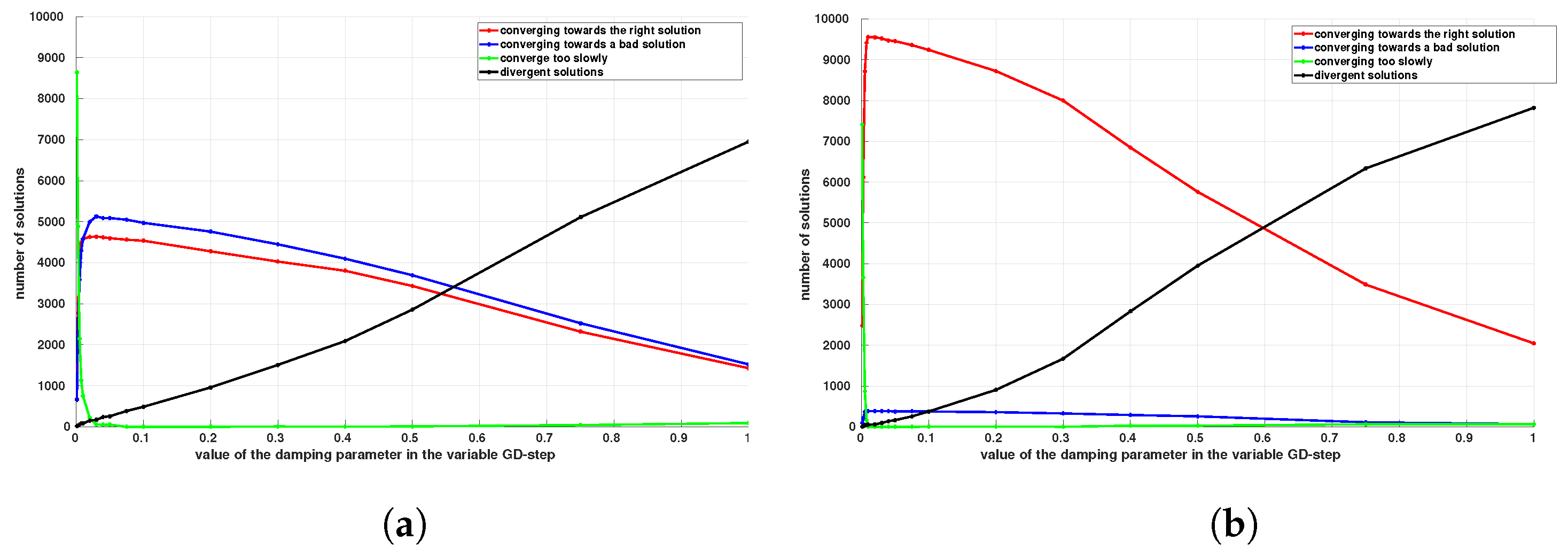
Further analysis of the adaptive step descent is carried out in Figure 7, revealing different cases of convergence of the algorithm: (i) the algorithm converges towards the correct estimate; (ii) the algorithm converges towards an erroneous estimate corresponding to a local minimum; (iii) the algorithm does not have time to converge and reaches the maximum number of iterations; and finally, (vi) the algorithm diverges. The results in Figure 7 are given for the estimation problem (5), including position and measurement errors, based on measurements acquired from 4 and 10 neighboring nodes, but similar results have been observed for the other cases. They clearly indicate the importance of increasing the number of measurements to improve the convergence of the algorithm to correct solutions. Convergence to local minima solutions is greatly reduced when using a significant number of relative measurements in the estimation. A clear improvement can be noticed when the damping parameter is used in the gradient descent step. It should be noted that the number of situations where the slow convergence of the algorithm does not lead to any solution is very limited except for very small values of the damping parameter which will obviously not be used. These results clearly show the relevance of introducing a damping parameter whose value could be suitably chosen according to the number of measurements available or desired for the estimation.

Finally, more detailed and comparative results revealing the average behavior over 10,000 simulations of each multilateration formulation scenario are summarized in

Table 2. Comparative localization results using the different formulations of the estimation problem, based on 4 relative measurements, with and without taking into account uncertainty models.

Localization Results Based on 4 Relative Measurements
Method	Convergence Rate	Localization Error (m)	Number of Iterations	Computation Time (ms)
Fixed-step GD/Equation (3) (w/o errors)	77.6%	0.0328 ± 0.0381	49.4 ± 49.9	0.14 ± 0.155
Variable-step GD/Equation (3) (w/o errors)	74.2%	0.033 ± 0.038	345 ± 358	3.2 ± 3.3
Fixed-step GD/Equation (4) (w/o errors)	72.0%	0.0003 ± 0.0004	2881 ± 2363	11.1 ± 9.1
Variable-step GD/Equation (4) (w/o errors)	63.3%	0.0005 ± 0.0014	1701 ± 2229	5.0 ± 6.7
Fixed-step GD/Equation (5) (w/errors)	76.6%	0.0517 ± 0.0374	49.4 ± 50.3	0.134 ± 0.147
Variable-step GD/Equation (5) (w/errors)	72.9%	0.055 ± 0.038	350 ± 370	3.0 ± 3.1
Fixed-step GD/Equation (6) (w/errors)	71.2%	0.051 ± 0.028	2795 ± 2266	6.7 ± 6.4
Variable-step GD/Equation (6) (w/errors)	63%	0.053 ± 0.030	1647 ± 2146	5.6 ± 7.3

,

Table 3. Comparative localization results using the different formulations of the estimation problem based on 5 relative measurements, with and without taking into account uncertainty models.

Localization Results Based on 5 Relative Measurements
Method	Convergence Rate	Localization Error (m)	Number of Iterations	Computation Time (ms)
Fixed-step GD/Equation (3) (w/o errors)	93.0%	0.024 ± 0.033	46.4 ± 41.9	0.119 ± 0.110
Variable-step GD/Equation (3) (w/o errors)	88.9%	0.025 ± 0.033	544 ± 647	2.5 ± 3.1
Fixed-step GD/Equation (4) (w/o errors)	89.0%	0.0002 ± 0.0002	2796 ± 21.20	12.3 ± 9.7
Variable-step GD/Equation (4) (w/o errors)	72.2%	0.0002 ± 0.0003	1395 ± 1864	4.2 ± 5.6
Fixed-step GD/Equation (5) (w/errors)	90.5%	0.051 ± 0.032	45.9 ± 45.7	0.231 ± 0.247
Variable-step GD/Equation (5) (w/errors)	86.3%	0.053 ± 0.032	539 ± 651	2.8 ± 3.3
Fixed-step GD/Equation (6) (w/errors)	86.3%	0.063 ± 0.034	2672 ± 1992	5.1 ± 4.4
Variable-step GD/Equation (6) (w/errors)	70.0%	0.063 ± 0.036	1340 ± 1792	5.2 ± 6.8

,

Table 4. Comparative localization results using the different formulations of the estimation problem based on 6 relative measurements, with and without taking into account uncertainty models.

Localization Results Based on 6 Relative Measurements
Method	Convergence Rate	Localization Error (m)	Number of Iterations	Computation Time (ms)
Fixed-step GD/Equation (3) (w/o errors)	96.3%	0.014 ± 0.017	38.0 ± 31.2	0.107 ± 0.051
Variable-step GD/Equation (3) (w/o errors)	95.7%	0.015 ± 0.017	1281 ± 1282	12.7 ± 13.5
Fixed-step GD/Equation (4) (w/o errors)	95.4%	0.0001 ± 0.0001	2105 ± 1649	5.3 ± 5.2
Variable-step GD / Problem (4) (w/o errors)	88.0%	0.0001 ± 0.0002	1239 ± 1633	7.0 ± 10.4
Fixed-step GD/Equation (5) (w/errors)	95.3%	0.059 ± 0.029	38.3 ± 33.4	0.116 ± 0.104
Variable-step GD/Equation (5) (w/errors)	94.2%	0.060 ± 0.030	1261 ± 1281	7.9 ± 8.0
Fixed-step GD/Equation (6) (w/errors)	95.5%	0.069 ± 0.034	2121 ± 1673	2.5 ± 2.4
Variable-step GD/Equation (6) (w/errors)	87.2%	0.071 ± 0.036	1232 ± 1644	9.9 ± 13.1

,

Table 5. Comparative localization results using the different formulations of the estimation problem based on 7 relative measurements, with and without taking into account uncertainty models.

Localization Results Based on 7 Relative Measurements
Method	Convergence Rate	Localization Error (m)	Number of Iterations	Computation Time (ms)
Fixed-step GD/Equation (3) (w/o errors)	98.9%	0.008 ± 0.006	27.1 ± 18.5	0.076 ± 0.051
Variable-step GD/Equation (3) (w/o errors)	95.5%	0.008 ± 0.006	232 ± 228	1.5 ± 1.4
Fixed-step GD/Equation (4) (w/o errors)	99.7%	0.0001 ± 0.0001	1522 ± 1407	6.3 ± 5.9
Variable-step GD/Equation (4) (w/o errors)	90.0%	0.0000 ± 0.0001	1032 ± 1404	3.9 ± 5.3
Fixed-step GD / Problem (5) (w/errors)	99.3%	0.069 ± 0.029	28.0 ± 21.4	0.115 ± 0.121
Variable-step GD/Equation (5) (w/errors)	95.5%	0.071 ± 0.029	235 ± 225	2.7 ± 2.6
Fixed-step GD/Equation (6) (w/errors)	97.4%	0.078 ± 0.034	1466 ± 1306	2.8 ± 3.3
Variable-step GD/Equation (6) (w/errors)	88.0%	0.079 ± 0.033	982 ± 1337	8.6 ± 11.6

,

Table 6. Comparative localization results using the different formulations of the estimation problem based on 8 relative measurements, with and without taking into account uncertainty models.

Localization Results Based on 8 Relative Measurements
Method	Convergence Rate	Localization Error (m)	Number of Iterations	Computation Time (ms)
Fixed-step GD/Equation (3) (w/o errors)	100.0%	0.006 ± 0.004	31.5 ± 15.6	0.066 ± 0.032
Variable-step GD/Equation (3) (w/o errors)	95.7%	0.006 ± 0.004	237 ± 178	1.7 ± 1.3
Fixed-step GD/Equation (4) (w/o errors)	100.0%	0.0000 ± 0.0000	2038 ± 1441	7.1 ± 5.6
Variable-step GD/Equation (4) (w/o errors)	90.0%	0.0000 ± 0.0000	775 ± 1138	3.1 ± 4.4
Fixed-step GD/Equation (5) (w/errors)	100.0%	0.091 ± 0.032	31.7 ± 15.9	0.133 ± 0.065
Variable-step GD/Equation (5) (w/errors)	95.9%	0.09 ± 0.032	239 ± 185	1.7 ± 1.3
Fixed-step GD/Equation (6) (w/errors)	100.0%	0.099 ± 0.039	2050 ± 1462	6.6 ± 5.0
Variable-step GD/Equation (6) (w/errors)	90.0%	0.099 ± 0.039	791 ± 1183	6.8 ± 10.2

,

Table 7. Comparative localization results using the different formulations of the estimation problem based on 9 relative measurements, with and without taking into account uncertainty models.

Localization Results Based on 9 Relative Measurements
Method	Convergence Rate	Localization Error (m)	Number of Iterations	Computation Time (ms)
Fixed-step GD/Equation (3) (w/o errors)	100.0%	0.005 ± 0.003	28.0 ± 15.4	0.066 ± 0.036
Variable-step GD/Equation (3) (w/o errors)	95.5%	0.005 ± 0.003	249 ± 218	3.3 ± 2.8
Fixed-step GD/Equation (4) (w/o errors)	100.0%	0.0000 ± 0.0000	1801 ± 1296	7.7 ± 5.8
Variable-step GD/Equation (4) (w/o errors)	91.5%	0.0000 ± 0.0000	779 ± 1263	3.5± 5.6
Fixed-step GD/Equation (5) (w/errors)	97.2%	0.108 ± 0.035	27.7 ± 15.3	0.095 ± 0.054
Variable-step GD/Equation (5) (w/errors)	93.4%	0.108 ± 0.035	247 ± 212	1.6 ± 1.4
Fixed-step GD/Equation (6) (w/errors)	92.0%	0.113 ± 0.041	1715 ± 1237	5.9 ± 5.1
Variable-step GD/Equation (6) (w/errors)	84.6%	0.113 ± 0.041	692 ± 1112	6.0 ± 9.7

and

Table 8. Comparative localization results using the different formulations of the estimation problem based on 10 relative measurements, with and without taking into account uncertainty models.

Localization Results Based on 10 Relative Measurements
Method	Convergence Rate	Localization Error (m)	Number of Iterations	Computation Time (ms)
Fixed-step GD/Equation (3) (w/o errors)	100.0%	0.004 ± 0.005	22.6 ± 15.5	0.066 ± 0.043
Variable-step GD/Equation (3) (w/o errors)	96.6%	0.004 ± 0.005	233 ± 173	1.5 ± 1.2
Fixed-step GD/Equation (4) (w/o errors)	100.0%	0.0000 ± 0.0000	1237 ± 1006	5.6 ± 5.3
Variable-step GD/Equation (4) (w/o errors)	94.0%	0.0000 ± 0.0000	526 ± 810	1.5 ± 2.3
Fixed-step GD/Equation (5) (w/errors)	92.3%	0.130 ± 0.032	22.9 ± 16.7	0.076 ± 0.055
Variable-step GD/Equation (5) (w/errors)	88.9%	0.130 ± 0.032	240 ± 177	1.8 ± 1.3
Fixed-step GD/Equation (6) (w/errors)	82.0%	0.131 ± 0.040	1218 ± 1025	2.6 ± 3.0
Variable-step GD/Equation (6) (w/errors)	77.5%	0.131 ± 0.040	471 ± 681	4.2 ± 6.0

. They are compared with respect to the localization errors versus the ground truth positions of the nodes, the average rate of convergence, and the computation time for the different formulations of the estimation algorithms.

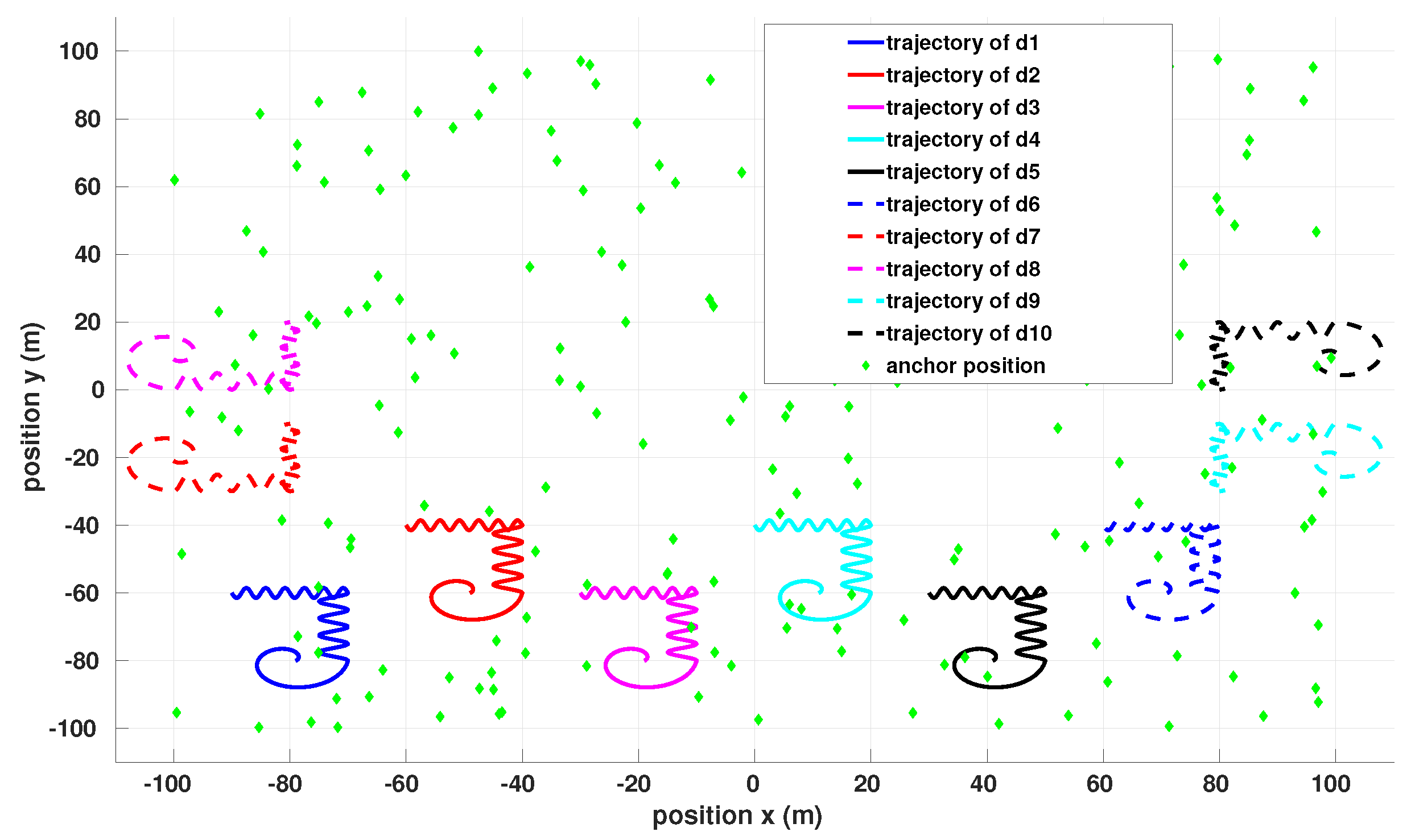
4.3. Towards Realistic Experimental Scenarios

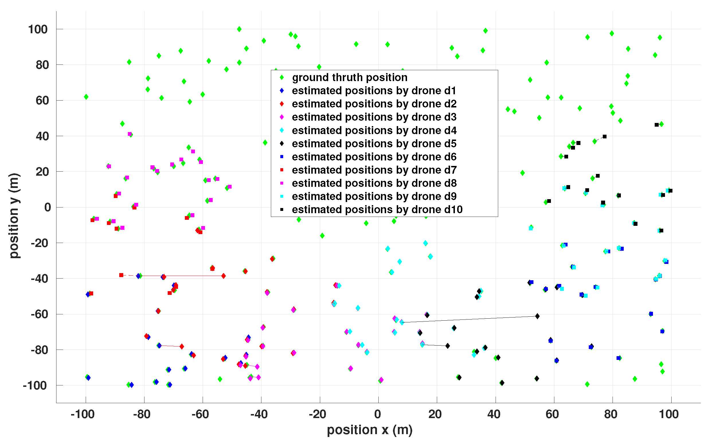
To conclude this study, we perform a realistic simulated scenario using a fleet of drones and a set of fixed anchors to evaluate the efficiency of solving the localization problem by multilateration of anchors and drones based on distance measurements. In this scenario (Figure 8), we consider 10 drones starting from different locations on the map. They are each equipped with an inertial measurement unit allowing us to obtain an odometry subject to significant errors, and an ultra-wideband sensor that can serve either as a track or as an anchor. The map is made up of 200 anchors of unknown positions scattered randomly across the map. Each drone executes a local trajectory and will therefore have the possibility of being within the range of certain anchors. The goal is to solve the twofold problem of locating as many anchors as possible, then to use the anchors located, to improve the odometric localization of the drones which is only given by inertial measurements.

Figure 9 shows the results of the estimated positions of the anchors detected by each drone, superimposed on the real positions (ground truth) on the initial map. One can observe a very small number of outliers compared to the number of well-located anchors. Some anchors have been located by different drones with small differences in their estimates. Interesting future work will be to merge and filter these different estimates to further improve the localization accuracy.

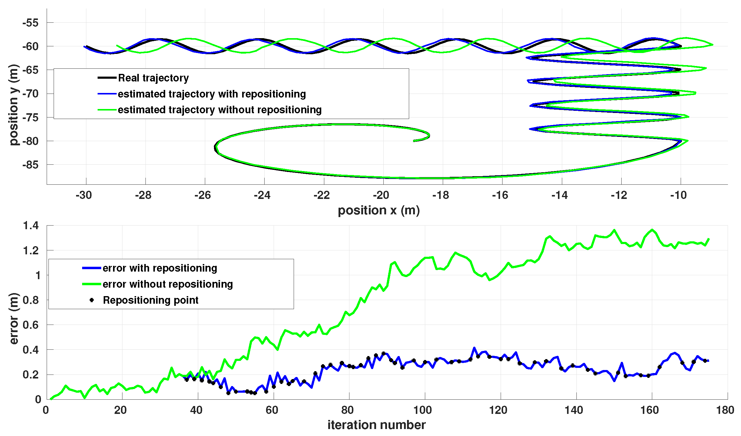
Figure 10 shows the results of an example drone localization scenario based on inertial measurements and enhanced by integrating distance measurements to anchors when they are located. The localization of each drone is first estimated by integrating the measurements of the inertial unit, which inevitably induces a strong drift depending on the distance traveled. The difficulty is therefore to take measurements at the start of the flight and to quickly locate a set of anchors before the drift and the localization error become too great to make multilateration unusable. When a sufficient number of anchors are located, the resolution of the multilateration localization optimization problem is re-initialized, which results in a significant improvement in the drone localization. The curves also indicate the localization errors in each case, with and without the use of the localized anchors to improve the drone localization. Points marked ’+’ on the blue curve indicate when anchor positions are made available and are therefore used to correct drift errors in inertial measurements, improving the localization accuracy. Note that the drone has no prior information on the location of the anchors. The positions of the detected anchors are first calculated with reference to the drone’s low-drift odometry; they are then exploited to correct the position of the drone, which explains the constant self-localization error. This process continues iteratively, which makes it possible to contain localization errors within a very limited interval.

5. Conclusions

This paper presents a unified formulation of the multilateration localization problem involving fixed sensors (anchors) and mobile agents (drones) based on ultra-wideband-range measurements. Different gradient descent methods have been studied, using a constant rate, a variable rate, and a new formulation introducing a damping parameter in the descent step. We have proposed a detailed study of the influence of various parameters such as the number of neighboring nodes for multilateration, the initialization of the algorithm, and the choice of the cost function, in addition to considering the positioning errors of the nodes and the sensor measurement noise. This leads, depending on the localization scenario, to parameter settings being chosen which allow for the best results according to the rate of convergence of the system, the localization error, and the computation time. In particular, the fixed-step gradient parameter can be set based on the number of neighboring nodes and produced good convergence and accuracy results in most scenarios. A thorough discussion is given based on extensive simulation results. The results have clearly shown good efficiency in locating anchors without prior knowledge of their positioning and, subsequently, the use of multilateration to perform drone tracking, thus improving its position given by the inertial unit. Trends of interest for future work include merging distributed estimates from multiple drones to further improve localization using global optimization, as well as carrying out experimental tests in real environments.

References

1. Valavanis, K.P.; Valavanis, K.P. Advances in Unmanned Aerial Vehicles: State of the Art and the Road to Autonomy, 1st ed.; Springer Publishing Company, Incorporated: New York, NY, USA, 2007. [Google Scholar]
2. Bouvry, P.; Chaumette, S.; Danoy, G.; Guerrini, G.; Jurquet, G.; Kuwertz, A.; Muller, W.; Rosalie, M.; Sander, J. Using heterogeneous multilevel swarms of UAVs and high-level data fusion to support situation management in surveillance scenarios. In Proceedings of the IEEE International Conference on Multisensor Fusion and Integration for Intelligent Systems, Baden-Baden, Germany, 19–21 September 2016; pp. 424–429. [Google Scholar]
3. Dehghan, S.M.M.; Farmani, M.; Moradi, H. Aerial localization of an RF source in NLOS condition. In Proceedings of the IEEE International Conference on Robotics and Biomimetics, Guangzhou, China, 11–14 December 2012; pp. 1146–1151. [Google Scholar]
4. Martinez Hernandez, L.A.; Perez Arteaga, S.; Sanchez Perez, G.; Sandoval Orozco, A.L.; Garcia Villalba, L.J. Outdoor location of mobile devices using trilateration algorithms for emergency services. IEEE Access 2019, 7, 52052–52059. [Google Scholar] [CrossRef]
5. Laclau, P.; Tempez, V.; Ruffier, F.; Natalizio, E.; Mouret, J.B. Signal-based self-organization of a chain of UAVs for subterranean exploration. Front. Robot. AI 2021, 8, 614206. [Google Scholar] [CrossRef] [PubMed]
6. Bekmezci, I.; Sahingoz, O.K.; Temel, S. Flying Ad-Hoc Networks (FANETs): A survey. Ad Hoc Netw. 2013, 11, 1254–1270. [Google Scholar] [CrossRef]
7. Yanmaz, E.; Costanzo, C.; Bettstetter, C.; Elmenreich, W. A discrete stochastic process for coverage analysis of autonomous UAV networks. In Proceedings of the IEEE Globecom Workshops, Miami, FL, USA, 6–10 December 2010; pp. 1777–1782. [Google Scholar]
8. Saeed, N.; Nam, H.; Al-Naffouri, T.Y.; Alouini, M.S. A state-of-the-Art survey on multidimensional scaling-based localization techniques. IEEE Commun. Surv. Tutorials 2019, 21, 3565–3583. [Google Scholar] [CrossRef] [Green Version]
9. Dieudonné, Y.; Labbani-Igbida, O.; Petit, F. Deterministic robot-network localization is hard. IEEE Trans. Robot. 2010, 26, 331–339. [Google Scholar] [CrossRef]
10. Hofmann-Wellenhof, B.; Lichtenegger, H.; Collins, J. Global Positioning System; Springer: Berlin/Heidelberg, Germany, 2001. [Google Scholar]
11. Teuliere, C.; Marchand, E.; Eck, L. 3-D model-based tracking for UAV indoor localization. IEEE Trans. Cybern. 2015, 45, 869–879. [Google Scholar] [CrossRef] [PubMed] [Green Version]
12. Herath, S.; Irandoust, S.; Chen, B.; Qian, Y.; Kim, P.; Furukawa, Y. Fusion-DHL: Wifi, imu, and floorplan fusion for dense history of locations in indoor environments. In Proceedings of the IEEE International Conference on Robotics and Automation (ICRA), Xi’an, China, 30 May–5 June 2021; pp. 5677–5683. [Google Scholar]
13. Vorst, P.; Sommer, J.; Hoene, C.; Schneider, P.; Weiss, C.; Schairer, T.; Rosenstiel, W.; Zell, A.; Carle, G. Indoor positioning via three different RF technologies. In Proceedings of the 4th European Workshop on RFID Systems and Technologies, Bremen, Germany, 10–11 June 2008; pp. 1–10. [Google Scholar]
14. Zhuang, Y.; Syed, Z.; Li, Y.; El-Sheimy, N. Evaluation of two WiFi positioning systems based on autonomous crowdsourcing of handheld devices for indoor navigation. IEEE Trans. Mob. Comput. 2016, 15, 14. [Google Scholar] [CrossRef]
15. Pakanon, N.; Chamchoy, M.; Supanakoon, P. Study on accuracy of trilateration method for indoor positioning with BLE beacons. In Proceedings of the 6th International Conference on Engineering, Applied Sciences and Technology, Chiang Mai, Thailand, 1–4 July 2020; pp. 1–4. [Google Scholar]
16. Bahl, P.; Padmanabhan, V.N. RADAR: An in-building RF-based user location and tracking system. In Proceedings of the IEEE INFOCOM, Tel Aviv, Israel, 26–30 March 2000; pp. 775–784. [Google Scholar]
17. Rusli, M.E.; Ali, M.; Jamil, N.; Din, M.M. An improved indoor positioning algorithm based on RSSI-trilateration technique for Internet of Things (IoT). In Proceedings of the International Conference on Computer and Communication Engineering, Kuala Lumpur, Malaysia, 6–8 September 2016; pp. 72–77. [Google Scholar]
18. Koohifar, F.; Kumbhar, A.; Guvenc, I. Receding horizon multi-UAV cooperative tracking of moving RF source. IEEE Commun. Lett. 2017, 21, 1433–1436. [Google Scholar] [CrossRef]
19. Heurtefeux, K.; Fabrice, V. De la pertinence du RSSI pour la localisation dans les réseaux de capteurs. In Proceedings of the AlgoTel, La Grande Motte, France, May 2012. [Google Scholar]
20. Yang, B.; Guo, L.; Guo, R.; Zhao, M.; Zhao, T. A Novel trilateration algorithm for RSSI-based indoor localization. IEEE Sens. J. 2020, 20, 8164–8172. [Google Scholar] [CrossRef]
21. Guvenc, I.; Chong, C.C. A survey on ToA based wireless localization and NLOS mitigation techniques. IEEE Commun. Surv. Tutorials 2009, 11, 107–124. [Google Scholar] [CrossRef]
22. Pradhan, S.; Pyun, J.Y.; Kwon, G.R.; Shin, S.; Hwang, S.S. Enhanced location detection algorithms based on time of arrival trilateration. In Proceedings of the 48th Asilomar Conference on Signals, Systems and Computers, Pacific Grove, CA, USA, 2–5 November 2014; pp. 1179–1183. [Google Scholar]
23. Nguyen, T.; Huynh, T.H. Experimental study of trilateration algorithms for ultrasound-based positioning system on QNX RTOS. In Proceedings of the IEEE International Conference on Real-time Computing and Robotics, Angkor Wat, Cambodia, 6–10 June 2016; pp. 210–215. [Google Scholar]
24. Wei, M.; Lihua, X.; Wendong, X. Decentralized TDoA sensor pairing in multihop wireless sensor networks. IEEE Signal Process. Lett. 2013, 20, 181–184. [Google Scholar]
25. Mekonnen, Z.W.; Slottke, E.; Luecken, H.; Steiner, C.; Wittneben, A. Constrained maximum likelihood positioning for UWB based human motion tracking. In Proceedings of the International Conference on Indoor Positioning and Indoor Navigation, Zurich, Switzerland, 15–17 September 2010; pp. 1–10. [Google Scholar]
26. Yassin, A.; Nasser, Y.; Awad, M.; Al-Dubai, A.; Liu, R.; Yuen, C.; Raulefs, R.; Aboutanios, E. Recent advances in indoor localization: A survey on theoretical approaches and applications. IEEE Commun. Surv. Tutorials 2017, 19, 1327–1346. [Google Scholar] [CrossRef] [Green Version]
27. Farooq-I-Azam, M.; Ni, Q.; Dong, M. An analytical model of trilateration localization error. In Proceedings of the IEEE Global Communications Conference, Big Island, HI, USA, 9–13 December 2019; pp. 1–6. [Google Scholar]
28. Pradhan, S.; Hwang, S.; Cha, H.; Bae, Y. Line Intersection Algorithm for the enhanced ToA trilateration technique. Int. J. Humanoid Robot. 2014, 11, 1442003. [Google Scholar] [CrossRef]
29. Hwang, S.; Shin, S. Advanced ToA trilateration algorithm for mobile localization. In Proceedings of the IEEE Asia-Pacific Conference on Antennas and Propagation, Auckland, New Zealand, 5–8 August 2018; pp. 543–544. [Google Scholar]
30. Farooq-I-Azam, M.; Ni, Q.; Dong, M. Extreme values of trilateration localization error in wireless communication systems. In Proceedings of the IEEE 31st Annual International Symposium on Personal, Indoor and Mobile Radio Communications, London, UK, 31 August–3 September 2020; pp. 1–6. [Google Scholar]
31. Larsson, M.; Larsson, V.; Astrom, K.; Oskarsson, M. Optimal trilateration is an eigenvalue problem. In Proceedings of the IEEE International Conference on Acoustics, Speech and Signal Processing, Brighton, UK, 12–17 May 2019; pp. 5586–5590. [Google Scholar]
32. Marinho, M.A.M.; Vinel, A.; Tufvesson, F.; Antreich, F.; Costa, J.P.C.L.D.; De Freitas, E.P. Spherical wave array based positioning for vehicular s cenarios. IEEE Access 2020, 8, 110073–110081. [Google Scholar] [CrossRef]
33. Fessler, J.A.; Hero, A.O. Space-alternating generalized expectation maximization algorithm. IEEE Trans. Signal Process. 1994, 42, 2664–2677. [Google Scholar] [CrossRef] [Green Version]
34. Beck, A.; Stoica, P.; Li, J. Exact and approximate solutions of source localization problems. IEEE Trans. Signal Process. 2008, 56, 1770–1778. [Google Scholar] [CrossRef]
35. Dogo, E.M.; Afolabi, O.J.; Nwulu, N.I.; Twala, B.; Aigbavboa, C.O. A comparative analysis of gradient descent-based optimization algorithms on convolutional neural networks. In Proceedings of the 2018 International Conference on Computational Techniques, Electronics and Mechanical Systems (CTEMS), Belagavi, India, 21–22 December 2018; pp. 92–99. [Google Scholar]
36. El-tanany, A.S.; Hussein, K.; Mousa, A.; Amein, A.S. Evaluation of Gradient Descent Optimization method for SAR Images Co-registration. In Proceedings of the 12th International Conference on Electrical Engineering (ICEENG), Cairo, Egypt, 7–9 July 2020; pp. 288–292. [Google Scholar]
37. Zhang, H.; Hager, W.W. A nonmonotone line search technique and its application to unconstrained optimization. SIAM J. Optim. 2004, 14, 1043–1056. [Google Scholar] [CrossRef] [Green Version]
38. Di Pietra, V.; Dabove, P.; Piras, M.; Lingua, A.L. Evaluation of positioning and ranging errors for UWB indoor applications. In Proceedings of the International Conference on Indoor Positioning and Indoor Navigation, Pisa, Italy, 30 September–3 October 2019; pp. 227–234. [Google Scholar]
39. Absil, P.A.; Mahony, R.; Andrews, B. Convergence of the iterates of descent methods for analytic cost functions. SIAM J. Optim. 2005, 16, 531–547. [Google Scholar] [CrossRef]
Figure 1. Multi-drone/anchor localization scenarios. (Left): A set of UWB tags with known positions are used to track a set of drones. (Right): A drone or a set of drones with estimated poses are used to retrieve unknown positions of a set of fixed UWB tags.
Applsci 13 01002 g001
Figure 2. Convergence results on 10,000 simulations using GD with fixed-step descent for estimation problems (3) (a) and (4) (b), respectively, without explicitly considering positioning and measurement error models and by varying the number of neighboring nodes from 4 to 10.
Applsci 13 01002 g002
Figure 3. Mean number of iterations to convergence with standard deviation on 10,000 simulations using GD with fixed-step descent for estimation problems (3) (a) and (4) (b), respectively, without explicitly considering position and measurement error models and by varying the number of neighboring nodes from 4 to 10.
Applsci 13 01002 g003
Figure 4. Convergence results on 10,000 simulations using GD with fixed-step descent for estimation problems (5) (a) and (6) (b), respectively, including position and range measurement error models and by varying the number of neighboring nodes from 4 to 10.
Applsci 13 01002 g004
Figure 5. Mean number of iterations to convergence with standard deviation on 10,000 simulations using GD with fixed-step descent for estimation problems (5) (a) and (6) (b), respectively, including position and range measurement error models and by varying the number of neighboring nodes from 4 to 10.
Applsci 13 01002 g005
Figure 6. Convergence results (left column) with the mean and standard deviations of the number of iterations until convergence (right column) over 10,000 simulations of the GD using variable-step descent as a function of the damping parameter, for estimation problems (3)–(6), with and without positioning and measurement error models and by varying the number of neighboring nodes from 4 to 10. (a) Problem (3) w/o errors; (b) Problem (3) w/o errors; (c) Problem (4) w/o errors; (d) Problem (4) w/o errors; (e) Problem (5) w/errors; (f) Problem (5) w/errors; (g) Problem (6) w/errors; (h) Problem (6) w/errors.
Applsci 13 01002 g006
Figure 7. Analysis of convergence results over 10,000 simulations using the adaptive gradient descent for estimation problem (5) including position and measurement error models, based on the measurements from 4 and 10 neighboring nodes, respectively. The red curves show the number of correct estimates, the blue curves correspond to the number of estimates corresponding to local minima, and the green and black curves correspond to non-convergence of the estimation due to reaching the maximum number of iterations (very slow convergence) or to the divergence of the estimation algorithm, respectively. Note that β = 1 corresponds to the classic formulation of variable-step gradient descent. (a) Based on 4 relative measurements; (b) Based on 10 relative measurements.
Applsci 13 01002 g007
Figure 8. Multi-drone and anchor localization scenario. Fixed anchors with unknown positions are marked with green dots. The ten drones and their local trajectories are represented using solid and dashed curves of different colors.
Applsci 13 01002 g008
Figure 9. Localization of anchors by a fleet of drones. The colors correspond to the different drones and the corresponding located anchors.
Applsci 13 01002 g009
Figure 10. Comparative localization results of one drone of the fleet. (Top): The trajectories estimated using only inertial odometry (green curve) and using inertial measurements and distance measurements to the anchors located by the drone (blue curve). The ground truth trajectory is represented by the dark curve. (Bottom): The Euclidean error of the localization in each case. Points marked ‘+’ on the blue curve indicate when multilateration is used in the estimation algorithm.
Applsci 13 01002 g010