Simulation and Validation of a Steering Control Strategy for Tracked Robots

Abstract

Tracked inspection robots have demonstrated their versatility in a wide range of applications. However, challenges arising from issues such as skidding and slipping have posed obstacles to achieving precise and efficient trajectory control. This paper introduces a method to determine the steering parameters of robot based on the surrounding obstacles and road information. The primary objective is to enhance the steering efficiency of tracked robots. The corresponding relationship between the track speed, driving force and track steering radius of the tracked robot is obtained. Considering the influence of track skid and slip, relationship models about the steering radius and traveling speed of the robot are established. The minimum and maximum steering radii in the obstacle avoidance process are analyzed, and a mathematical model of the relationship between the steering angle of the robot and the distance between the side obstacles is established. The trajectory deviation model of the tracked robot is established, and a principle analysis of the LiDAR ranging is completed. This lays the foundation for a steering measurement and control system for tracked robots. ADAMS(2020) software is used to establish the multi-body dynamics model of the tracked robot, and three different obstacle-avoiding steering control strategies are designed for the robot in a simulated environment with space obstacles. The simulation experiment demonstrates that the robot achieves more efficient obstacle avoidance steering through the use of differential steering, leading to a decrease in both track skid and slip rates. Through the simulation experiment, it can be seen that the robot uses differential steering to complete the obstacle avoidance steering movement more efficiently, and the track skid and slip rates are smaller. The simulation results are used to complete the steering control experiment of the tracked robot on different road surfaces. The results show that by adjusting the track driving parameters, the robot can effectively complete the obstacle-avoiding steering movement by using the differential steering control strategy, which verifies the accuracy of the steering control strategy.

1. Introduction

Tracked robots are widely used in various industries for inspection purposes [1,2]. Liu WJ et al. designed a triangular tracked regenerative rice harvester for use in agriculture [3]. Zhao J et al. engineered a compact, four-track articulated fire-extinguishing robot with four-wheel drive capability, enabling it to adeptly conduct fire detection and extinguishing operations within confined spaces and on challenging terrain [4]. Shafaei S. M. et al. pointed out that the traveling speed and payload of tracked vehicles have important effects on the motion and traction power efficiency of vehicles, and the sliding power efficiency of tracked vehicles mainly depends on the load weight [5]. It is difficult to achieve precise control of tracked robots, and one of the most challenging issues faced by the designers or manufacturers of these robots is accurately predicting their motion due to the complex and nonlinear interaction between the tracks and the terrain during skid-steering curves [6]. Chen TT et al. established a simplified geometric model of a tracked combine taking into account the influence of the header and track on headland turning, and concluded that the differential steering of a tracked combine can significantly improve work efficiency [7].

Researchers worldwide have undertaken comprehensive investigations into the steering mechanisms of tracked robots, considering the influence of track skip and slip. For example, Jia W et al. developed a dynamic model with high computational accuracy and studied the steering stability of tracked vehicles in sandy road environments under different conditions [8]. Xiong H., et al. proposed a new dynamic modeling method and motion control approach for a submarine tracked vehicle, proving its stability using Lyapunov theory [9]. Hu K., et al. compared the multi-body dynamics model of Recurdyn/Track with an established model to verify its accuracy in the time and frequency domains, considering the transient characteristics of orbit–ground contact [10]. Sabiha A.D et al. optimized the backstepping controller as a kinematic controller and verified the stability analysis of the entire system using Lyapunov theory [11]. Fang Y., et al. developed a dynamic model for a crawler-type wall-climbing robot with negative pressure adsorption, analyzing the influence of design parameters on its motion performance [12]. Ding, Z., et al. proposed a new method that can accurately test the slip coefficient of tracked vehicles under different ground conditions to reduce the influence of the slip coefficient of tracked vehicles on the steering process [13]. Wu, J.Q., et al. established a model that can reverse-calculate the current and voltage signals of tracked ATVs in a specific trajectory, so as to provide a theoretical basis for the trajectory control of tracked articulated vehicles [14].

The above literature Indicates that tracked robots are used in all industries. However, the steering control strategy of the tracked robot is different for different environments, traveling speeds, and structural parameters [15]. Therefore, it is necessary to formulate a robot driving control strategy based on the structural characteristics of the tracked robot, combined with road environment information and driving control requirements, and complete robot inspection tasks [16]. In this paper, we propose the development and simulation of a tracked robot steering control strategy in ADAMS software. Firstly, the body structure and related parameters of the tracked robot were introduced. Secondly, considering the influence of track skid and slip, relationship models about the steering radius and traveling speed of the robot were established in Matlab(2022b) software. The influence of the relative position change between the tracked robot and obstacle on the steering control of the robot was studied and analyzed, and corresponding steering control strategies were formulated. Thirdly, to achieve obstacle avoidance control for the inspection robot in a roadway environment, the sensing and signal processing layer, decision control layer, and motion execution control layer were established. The virtual prototype of the tracked robot and the simulation environment of the obstacle environment were established in ADAMS software, and the rationality of the control strategies of the tracked robot obstacle-avoiding steering were simulated and analyzed. Finally, the theoretical analysis results were used to guide the tracked robot to complete a performance test.

2. Analysis of Robot Structure and Steering Radius

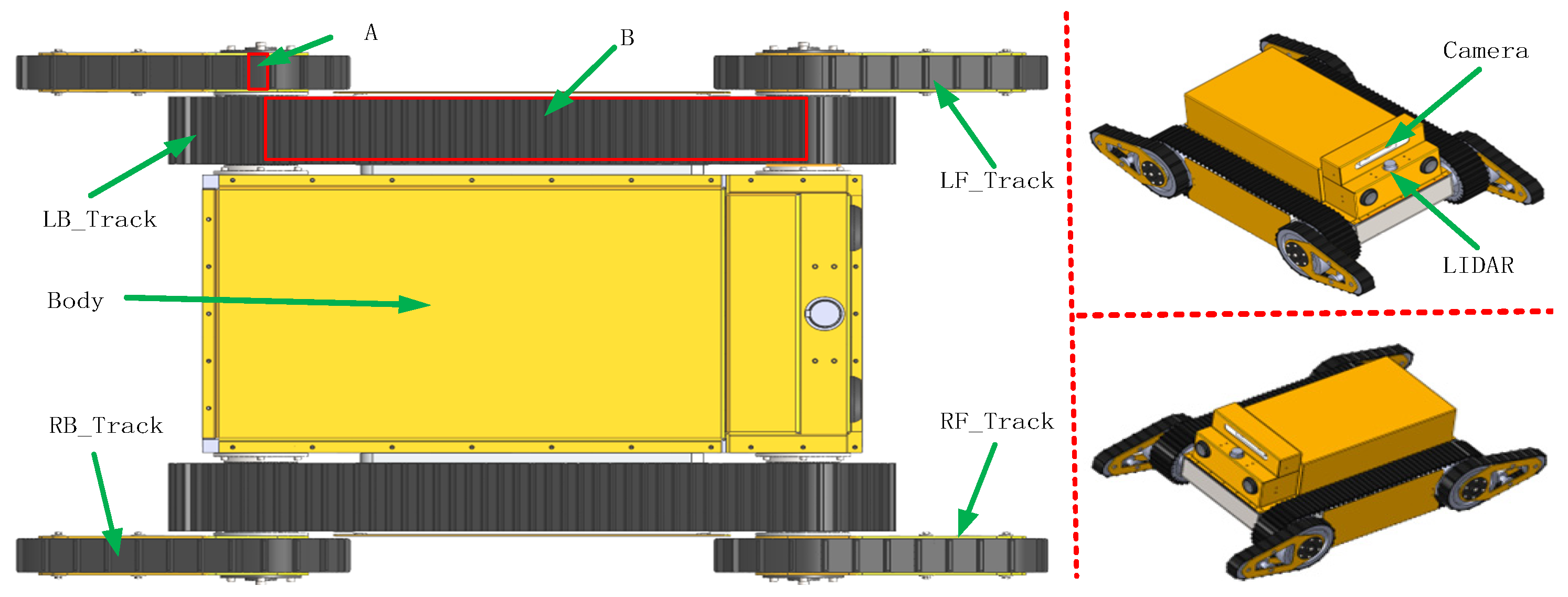
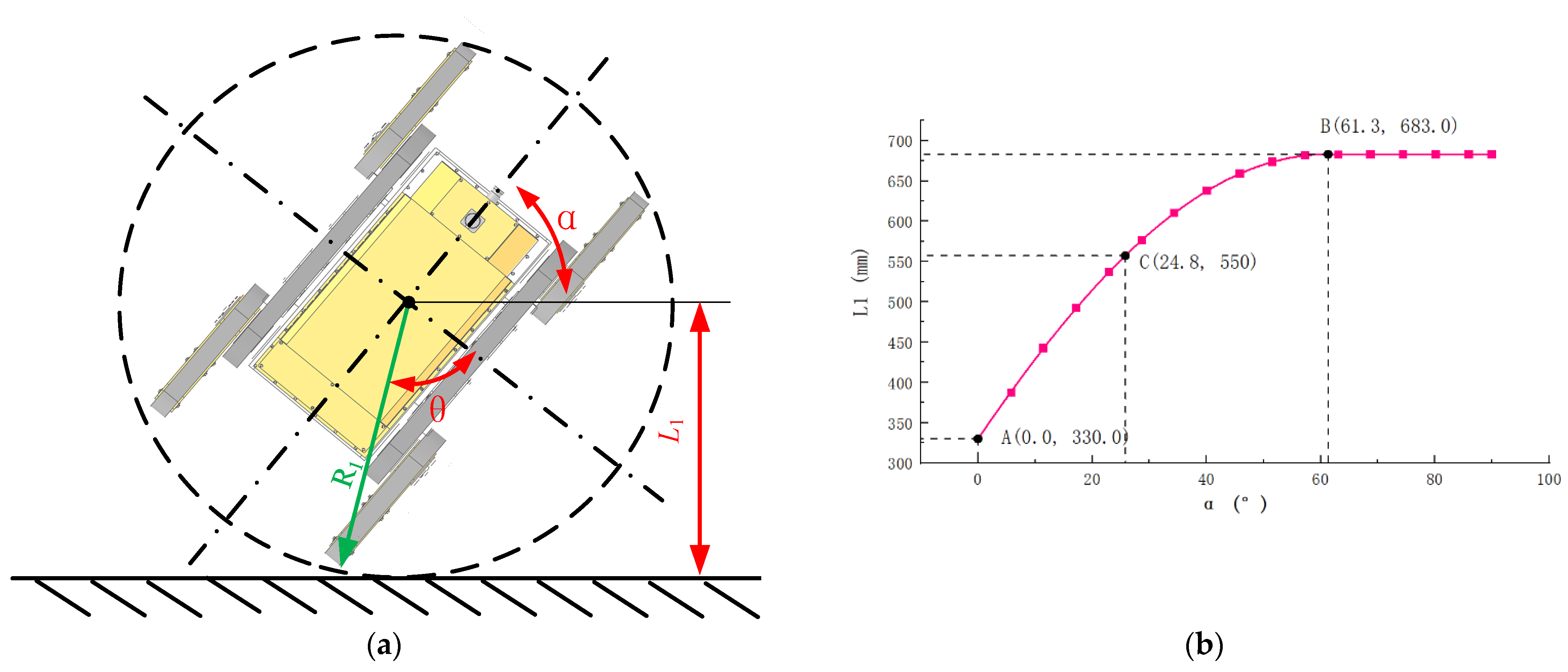
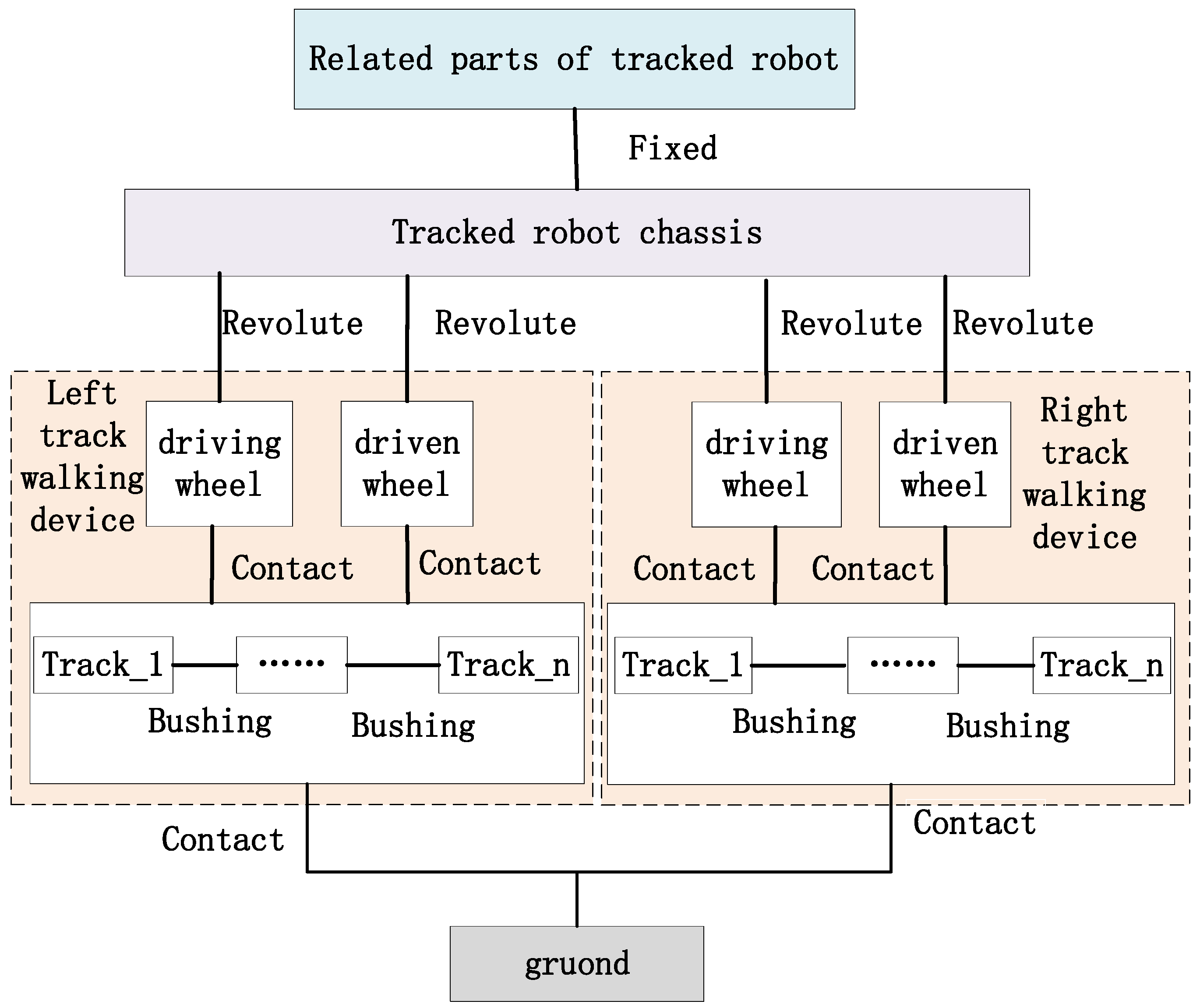
2.1. Analysis of Robot Structure

In this study, a tracked robot with four swinging arms and six tracks, which can perform routine inspection under complex terrain conditions, was used. The robot’s body structure is illustrated in Figure 1, based on previous work by this research group. The four swinging arms of the robot could rotate independently and freely. When the robot needs to cross an obstacle, it can complete the obstacle-surmounting tasks by controlling the rotation angle of its four swing arms [17]. When the robot is driving on a horizontal road surface, obstacle avoidance steering can be controlled by the speed difference between the two sides of the robot track. Based on an analysis of the structural parameters and steering radius of the robot, the traction force and resistance torque models of the tracked robot were established [18]. The current study is a continuation of previous studies by the authors focused on the obstacle-surmounting and obstacle avoidance performance of tracked robots. However, this study focuses on establishing the correlation between the steering radius, obstacle position, and track skid and slip of the tracked robot. The robot can autonomously devise its steering strategy by considering the relationship with obstacle positions and LiDAR measurement data, enabling swift and efficient steering.

When the robot is driving on a hard road, the contact area between the swing arm track and the road is small (Figure 1, area A), and is far smaller than the contact area between the main track and the ground (Figure 1, area B). Therefore, the influence of the swing arm track on the steering performance of the robot can be ignored. However, it is necessary to consider the influence of the swing arm track on steering performance when the robot is driving on a relatively soft road surface, because area A will be much larger, resulting in increased resistance. The main parameters of the tracked robot are shown in

Table 1. Main parameters of tracked robot [12].

Name	Value
Body weight (G)	1200 N
Body width (B)	790 mm
Body height (h)	360 mm
Wheelbase (L)	650 mm
Radius of driving wheel (Rw)	102 mm
Motor torque (T)	28.2 N.m
Inspection speed (v)	2 km/h
The width of swing arm (B0)	123 mm
The length of swing arm (Lb)	312 mm
Track width (b)	100 mm

.

2.2. Analysis of the Skid and Slip Rates

When the tracked robot is running, the speed performance of each point on the track is inconsistent. Through the speed analysis of each point on the track, the relationship between $v_j$, $v_q$, and $v_r$ can be obtained as shown in Figure 2. The expressions of $v_j$, $v_q$, and $v_r$ are established as follows:

$$v_j=\sqrt{v_r^2+v_q^2+2v_r{v}_q\cos \beta }$$

(1)

where $v_r$ is the winding velocity, that is, is the belt linear speed. $v_q$ is the traction velocity. $v_j$ is the absolute speed on the track and $\beta$ is the angle between $v_r$ and $v_q$.

When there was no skid or slip between the robot track and the ground, the velocities of the two points A and B were analyzed. At point A, $\beta =0$ and $\left|v_r\right|=\left|v_q\right|$, and $v_{jA}=2v_r$. At point B, $\beta =180°$ and $v_r=-v_q$, and $v_{jB}=0$, and the track remains stationary with the ground. When $\left|v_r\right|\ne \left|v_q\right|$, $v_{jC}=v_q-v_r\ne 0$. During $v_j<0$, the absolute velocity at point A is in the same direction as the winding velocity, and the robot produces a slipping phenomenon. During $v_j>0$, the absolute velocity at point B is opposite to the direction of the winding velocity, and the robot produces a skidding phenomenon.

According to the terramechanical models [19,20,21,22], the skid and slip rates of the robot track can be expressed as follows:

$$i=\left\{\begin{array}{l}\frac{{\nu }_r-{\nu }_j}{{\nu }_r}=\frac{{\nu }_q}{{\nu }_r}\times 100\%=i_s,if {\nu }_r\ge {\nu }_j\\ \frac{{\nu }_j-{\nu }_r}{{\nu }_r}=-\frac{{\nu }_q}{{\nu }_r}\times 100\%=i_t,if {\nu }_j>{\nu }_r\end{array}\right.$$

(2)

where $i_s$ is the slip rate, $i_t$ is the skid rate, and ${\nu }_j$ is the actual velocity at the center of the robot’s tracked wheel.

2.3. Relation between Driving Force and Slip Rate

When describing the skidding and slipping characteristics of a robot, it is necessary to assume that each point of the track cannot be stretched. That is, no deformation will occur. If the speed of each point on the track connected to the ground is the same, then the shear displacement of each point increases linearly. The relationship between x and j is shown in Figure 2. The expression j for the shear displacement of the track is given as follows:

$$j=ix$$

(3)

where $i$ is the skid or slip rate, and x is the distance between the track in contact with the ground and the endpoint of the track.

The formation of the track shear force is related to the shear displacement, so the distribution of the shear stress along the contact length can be determined. When the slip rate is given, the total driving force generated by the track can be obtained from the relationship between shear stress and shear displacement under the track, which can be calculated using the following formula:

$$F=b{\displaystyle {\int }_0^L\tau }dx=b{\displaystyle {\int }_0^L(c+p\tan \varphi )}(1-e^{-j/k})dx$$

(4)

where b is track width, $\tau$ is shear stress, p is the normal pressure, k is the shear displacement parameter, c is the ground cohesion, $\varphi$ is the internal shear resistance angle, and L is the wheelbase of the robot.

It can be seen from the above formula that the driving force of the track is related to the normal pressure distribution on the track contact surface. For a uniform normal pressure distribution, $p=G/bL$, the total driving force of the track is determined using the following formula.

$$F=bcL+G\tan \varphi \left[1-\frac{k}{iL}(1-e^{-iL/k})\right]$$

(5)

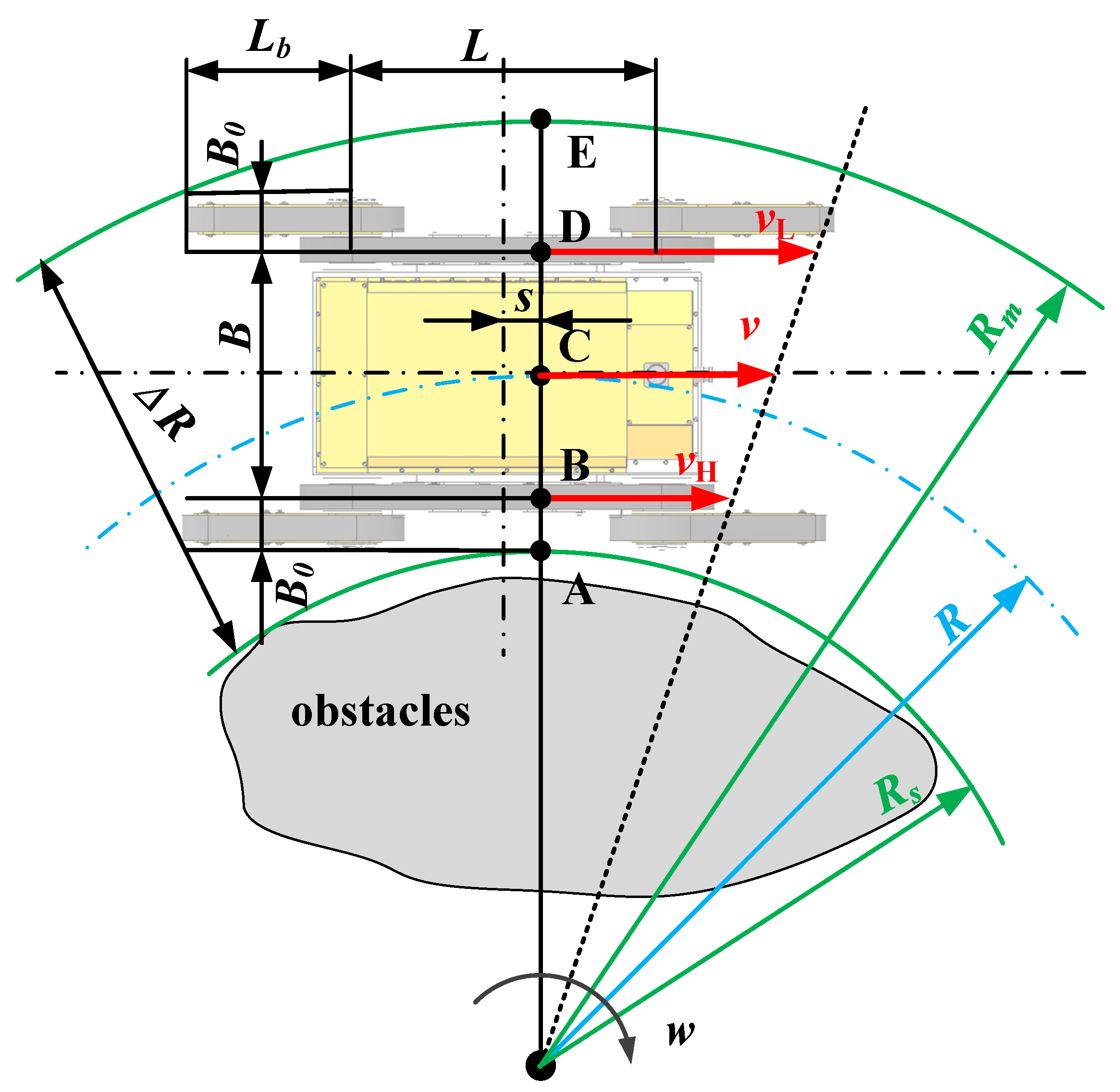
2.4. Analysis of Tracked Robot Steering Radius

In the process of steering, owing to the influence of track skid and slip, the track with higher speed will be affected by sliding resistance, and its speed will be reduced. On the contrary, the track with lower speed will be affected by the sliding traction force, and its speed will increase. v is the speed of the robot. $v_R^{\prime }$ and $v_L^{\prime }$ are the theoretical speeds of the right and left tracks, respectively, and $v_R$ and $v_L$ are the actual speeds of the right and left tracks, respectively. $v_R={\omega }_{R}r$ and $v_L={\omega }_{L}r$, where ${\omega }_R$ and ${\omega }_{\mathrm{L}}$ are the rotational speeds of the right and left driving wheels, respectively. The theoretical Instantaneous Center of Rotation (ICR′) is inconsistent with the actual Instantaneous Center of Rotation (ICR), as shown in Figure 3. The turning radius of a tracked robot can be described by the following formula:

$$\left\{\begin{array}{l}R=\frac{v_{\mathrm{R}}+v_{\mathrm{L}}}{v_{\mathrm{R}}-v_{\mathrm{L}}}=\frac{{\omega }_{\mathrm{R}}+{\omega }_{\mathrm{L}}}{{\omega }_{\mathrm{R}}-{\omega }_{\mathrm{L}}}\\ R\prime =\frac{v{\prime }_{\mathrm{R}}+v{\prime }_{\mathrm{L}}}{v{\prime }_{\mathrm{R}}-v{\prime }_{\mathrm{L}}}=\frac{\omega {\prime }_{\mathrm{R}}+\omega {\prime }_{\mathrm{L}}}{\omega {\prime }_{\mathrm{R}}-\omega {\prime }_{\mathrm{L}}}\\ \rho =R/B\\ \rho \prime =R\prime /B\end{array}\right.$$

(6)

where R is the actual turning radius, and R′ is the theoretical turning radius, $\rho$ is the actual relative steering radius, and $\rho \prime$ is the theoretical relative steering radius. B is the width of the robot body.

Considering the slip and skid of two tracks, the relationship between the actual speed $v$ and relative steering radius $\rho$ of the tracked robot can be obtained as follows:

$$\left\{\begin{array}{l}v=\frac{1}{2}\left[w_{R}r(1-i_R)+w_{L}r(1-i_L)\right]\\ \rho =\frac{w_R(1-i_R)+w_L(1-i_L)}{w_R(1-i_R)-w_L(1-i_L)}\end{array}\right.$$

(7)

where $w_R$ is the angular velocity of the right track and $w_L$ is the angular velocity of the left track. $i_R$ and $i_L$ are the slip rates of the right and left tracks, respectively.

3. Relationship between Robot Steering Radius and Obstacle Position

To understand the relationship between the robot’s motion trajectory and obstacles, a plane motion analysis diagram is shown in Figure 4. $R_m$ represents the maximum radius of the arc traversed by the robot during steering. Similarly, $R_s$ denotes the minimum radius of the arc traversed by the robot during steering. The minimum space required for the robot to travel was a plane composed of two arcs, namely $R_m$ and $R_s$, and the distance between the two arcs was $\Delta R$. Therefore, if the roadway width is greater than $\Delta R$, the robot can successfully avoid obstacles without colliding with them. From Figure 5, the following equation is obtained:

$$\left\{\begin{array}{l}\frac{R_s+B_0+B}{R_s+B_0}=\frac{v_L(1-i_L)}{v_R(1-i_R)}=k\\ R_m^2={\left(R_s+2B_0+B\right)}^2+{\left(L/2+L_b+s\right)}^2\end{array}\right.$$

(8)

where k is the ratio of the speed of the left track to the right track. s is the offset distance of the robot’s center of gravity. B₀ is the distance from the center of the track to the outside of the swing arm. Therefore, the calculation formula of $R_s$ and $R_m$ is as follows:

$$\left\{\begin{array}{l}{R}_s=\frac{B_0}{k-1}-B\ge 0\\ R_m=\sqrt{{\left(\frac{B}{k-1}+B_0+B\right)}^2+{\left(L/2+L_b+s\right)}^2}\end{array}\right.$$

(9)

Assuming that the swing arm of the robot is unfolded when it performs a steering motion, the robot must maintain a certain distance from the obstacles to realize steering. According to the relationship between robot structure and size, $\alpha$, $\theta$ and $R_1$ can be obtained as follows:

$$\left\{\begin{array}{l}{L}_1=R_1\cos (\theta -\alpha )\\ R_1=\sqrt{{\left(L+2L_b\right)}^2+{\left(B+2B_0\right)}^2}/2\\ \tan \theta =\frac{L+2L_b}{B+2B_0}\end{array}\right.$$

(10)

where $L_1$ is the distance between the center of the robot and the side obstacles, $\alpha$ is the yaw angle, and $\theta$ is the structural angle, $R_1$ is the structural radius of the robot center steering.

By substituting the structural parameters of the tracked robot from Table 1 into Equation (10), the relationship between the robot’s distance from the side obstacle and its steering angle can be calculated using Matlab software. The relationship between the maximum steering angle of the robot and the positions of the lateral obstacles is shown in Figure 5a, the dotted circle in the figure represents the space required for the robot to turn in place. When the distance between the center of the robot and the lateral obstacles is L₁ = 330 mm, the robot cannot turn and can only drive forward, as shown at point A of Figure 5b. When L₁ = 550 mm, the maximum steering angle of the robot is 24.8°, as shown at point C in Figure 5b. When L₁ = 683 mm, the maximum steering angle of the robot is 61.3°, as shown at point B of Figure 5b. When L₁ > 683 mm, the robot can turn freely and is not restricted by obstacles.

4. Deviation Correction Control Method of Tracked Robot

4.1. Control Mechanism of Deviation Correction

The geodetic coordinate system is XOY, the robot body coordinate system is xoy, the current position coordinate of the robot is (x₁, y₁), and the target position coordinate is (x₂, y₂). $\alpha$ is the yaw angle, as shown in Figure 6. ${\alpha }_e$ is the angular deviation. x_e and y_e are, respectively, the deviation of the target position in the x and y directions under the robot body coordinate system; ∆X and ∆Y are, respectively, the deviation under the x and y directions under the geodetic coordinate system. Then, the position error $p_e$ in the robot body coordinate system can be expressed as

$$p_e=\left[\begin{array}{l}{x}_e\\ y_e\\ {\alpha }_e\end{array}\right]=\left[\begin{array}{ccc}\cos {\alpha }_e& \sin {\alpha }_e& 0\\ -\sin {\alpha }_e& \cos {\alpha }_e& 0\\ 0& 0& 1\end{array}\right]\left[\begin{array}{c}\Delta X\\ \Delta Y\\ \Delta \alpha \end{array}\right]$$

(11)

Using the trajectory error of the robot, the trajectory tracking control of the robot can be realized by adjusting the speed difference of the tracks on both sides of the robot.

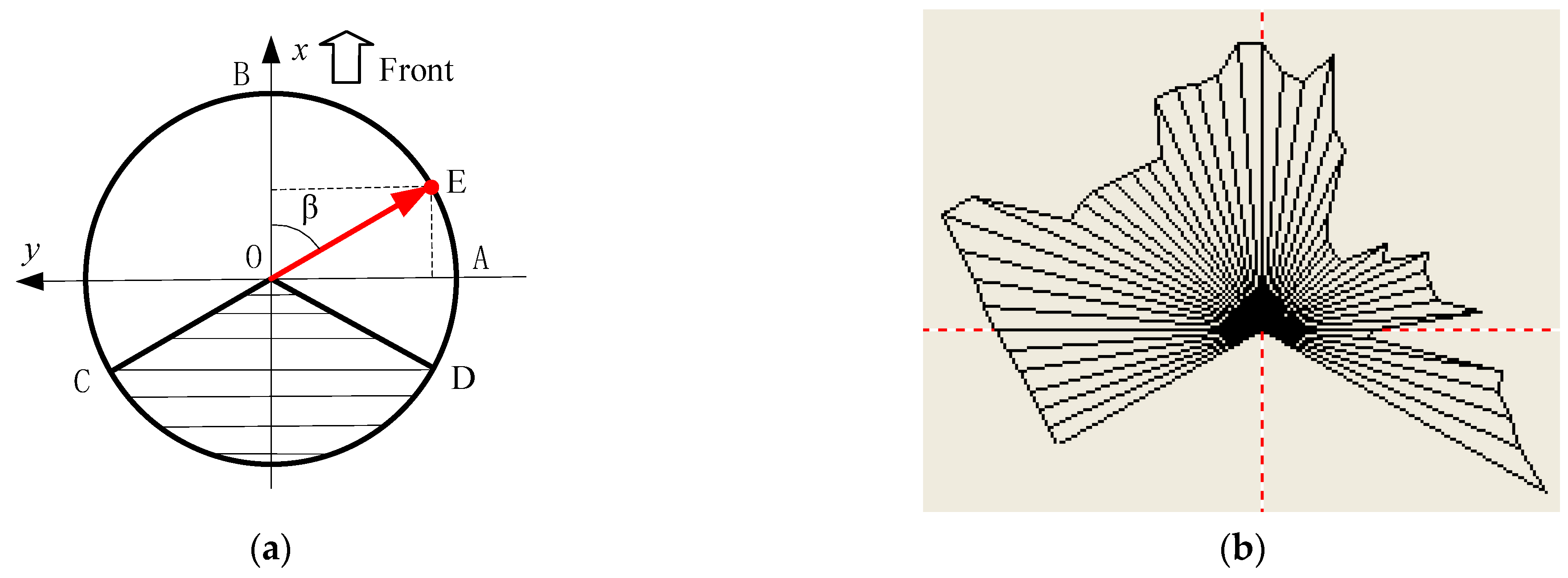
4.2. Principle Analysis of LiDAR Ranging

The inspection robot uses a two-dimensional laser LiDAR for ranging. The laser radar uses a laser beam of 768 nm wavelength, and the measuring method adopts the principle of TOF (time of flight). During the detection process of the robot, the LiDAR can collect obstacle data in 683 directions per scanning cycle, and the detection range is between −120° and +120°. The definition of data points is shown in Figure 7a; the shaded part in the figure is the detection blind area of the robot. The obstacle detection interface is depicted in Figure 7b, with the software program developed in a VC++ environment. LiDAR is used as the coordinate system origin to measure the surrounding obstacles, and the counterclockwise rotation of point B is positive. The distance of point E from the LiDAR is OE, expressed by $\rho$. Then, the distance between any point on the DBC arc and the LiDAR can be calculated using the following formula.

$$\left\{\begin{array}{l}x=\rho \cos \beta \\ y=\rho \sin \beta \end{array}\right., \beta =\pm 120°$$

(12)

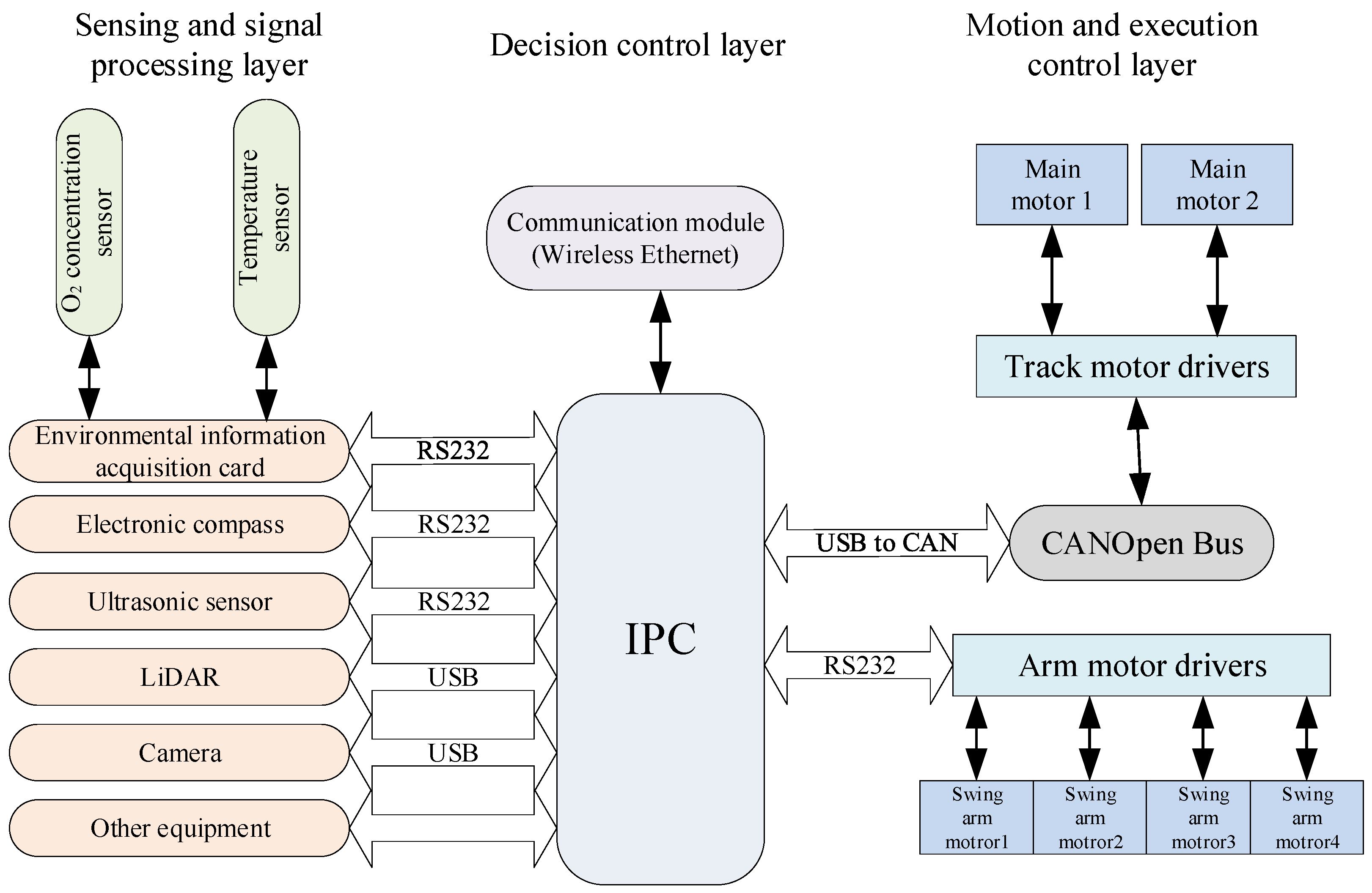
4.3. Robot Measurement and Control System

To achieve obstacle avoidance control for inspection robots in a roadway environment, it is essential to establish a measurement and control system using LiDAR. This system enables the robot to compute its turning radius based on the obstacle distance information gathered by LiDAR. The inspection robot adopts a distributed and modular approach to build the inspection robot measurement and control system. The system is divided into three levels, namely, a sensing and signal processing layer, a decision control layer, and a motion execution control layer. Figure 8 shows the overall structure of the inspection robot measurement and control system.

The sensor and signal processing layer uses multiple sensors to monitor the internal state and external environment information of the robot, and uploads the collected data to the IPC (Industrial Personal Computer) of the decision control layer through their respective conditioning circuits and communication buses. The main function of the decision control layer is to fuse the data of each sensor and then convert the processing result into the command of the motion execution control layer. The motion executive control layer is mainly composed of a driver and a motor. By controlling the movement of two main track motors and four swing arm motors, the combination of various actions of multiple motors can realize the robot’s forward, backward, turning, obstacle avoidance, and other behaviors. Through the three levels of the measurement and control subsystems, the coordination of the inspection robot is achieved to complete various tasks.

5. Simulation Analysis of Obstacle Avoidance Steering Control

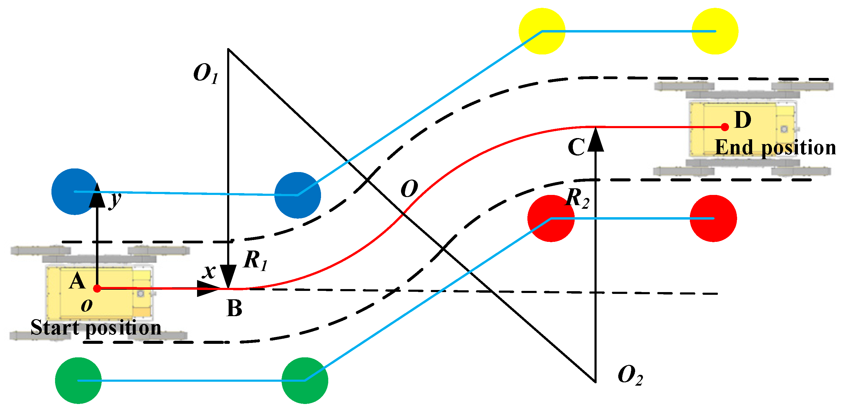
5.1. Obstacle Avoidance Steering Control Strategy for Tracked Robot

As shown in Figure 9, there are multiple paths for the robot to choose during the obstacle-avoiding steering movement from point A to point B, and there will be no collision with the surrounding obstacles during this process. For example, the robot realizes obstacle avoidance steering movement through center steering and differential steering, as shown in Figure 9. Center steering refers to a tracked robot’s maneuver where one side of the tracks moves forward while the other side moves backward at the same speed, causing the robot to rotate around its own center. Typically, this method requires the robot to come to a halt before executing center steering and is commonly used when the robot needs to make sharp turns in extremely confined spaces. Differential steering, on the other hand, involves a tracked robot changing its direction by altering the speed difference between the two tracks while keeping both tracks in continuous motion. This allows the robot to maintain its movement without stopping and is suitable for making turns in more spacious environments.

In the process of center steering movement, the robot can reach point B from point A through two executions of center steering, that is, the robot rotates counterclockwise at point C and clockwise at point D, and the trajectory of the robot is ACDB, as shown in strategy 1 in Figure 9. Similarly, the robot can get from point A to point B through four center turns, and the trajectory of the robot is AEFGHB, as shown in strategy 2 in Figure 9. In the differential steering motion, the robot completes the obstacle-avoiding steering movement through two differential steering movements, and the steering trajectory of the robot is AKOJLB, as shown in strategy 3 in Figure 9.

Trajectory ACDB: The steering angle of the robot at point C can be calculated using the following formula, where clockwise rotation of the robot is negative, counterclockwise rotation is positive, and the steering angle of the robot at point D is opposite to the steering angle of the robot at point C.

$$\angle DC{o}_2=\arctan \frac{D_{\mathrm{y}}-C_{\mathrm{y}}}{D_{\mathrm{x}}-C_{\mathrm{x}}}$$

(13)

Trajectory AEFGHB: The steering angle of the robot at point E can be calculated using the following formula. Points F, G, and H can be calculated using the similarity formula.

$$\angle FE{o}_2=\arctan \frac{F_{\mathrm{y}}-E_{\mathrm{y}}}{F_{\mathrm{x}}-E_{\mathrm{x}}}$$

(14)

Trajectory AKOJLB: The steering radii of the robot are $O_{1}O$ and $O{O}_2$, respectively. When the steering radius of the robot is equal at the two stages of the steering process, the O point is on the midpoint of $O_1{O}_2$, that is, $O_{1}O=O{O}_2=R$, then $OM=O_{2}K/2$ and $O_{1}M=O_{1}K/2=R/2$. The following formula can be derived from the right triangle $O_{1}MO$ relation:

$$O_{1}O=O_1{M}^2+O{M}^2$$

(15)

The robot steering radius formula can be obtained by simplifying the formula as follows:

$$R=\frac{\sqrt{3}}{3}{O}_{2}K$$

(16)

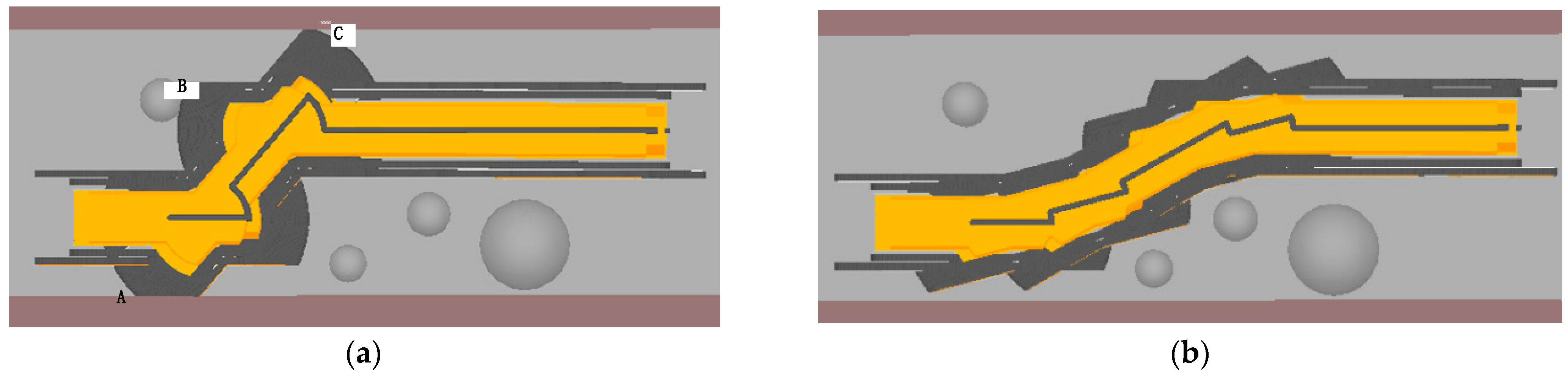
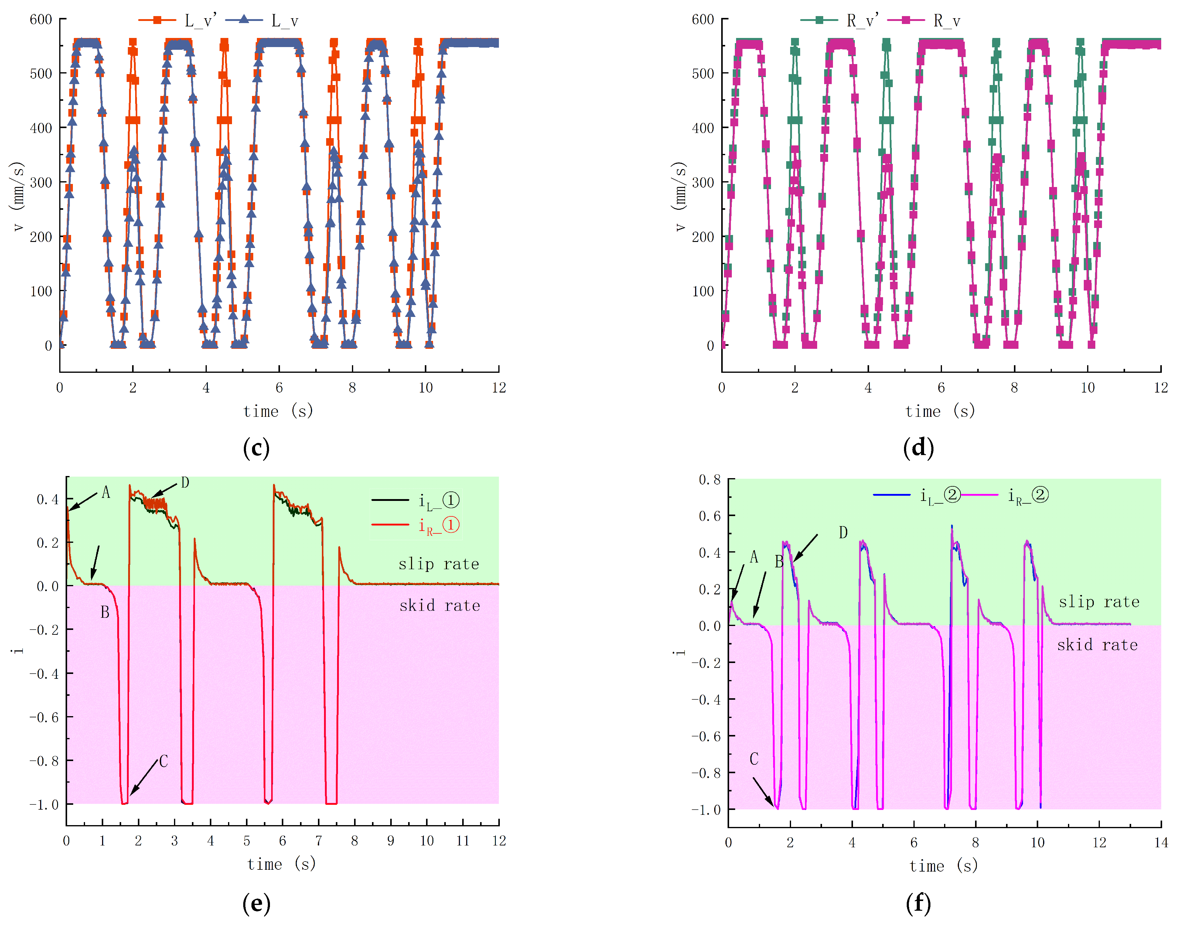
5.2. Center Steering Simulation Analysis

To investigate how the robot’s steering performance is affected by its three steering control strategies, this study utilizes SolidWorks 3D software to construct the robot model. Subsequently, ADAMS(2020) software is employed to impose appropriate constraints on the relevant components of the robot. Figure 10 illustrates the interconnections among the robot’s components. The simulation experiments of obstacle avoidance control were completed according to the control requirements by editing the driving function of the robot’s obstacle avoidance motion control.

In this study, the distance from the side obstacles was 550 mm. Based on the position relationship between the robot and obstacles, two schemes of center steering were set for the robot, in which the robot needed to stop and start several times. Strategy 1 does not consider the positional relationship between the robot and obstacles and the length of the robot swing arm; the robot completed the obstacle avoidance steering control by adjusting the motor parameters twice. Although strategy 2 considers the relevant influencing factors, the robot completed the obstacle avoidance steering control by adjusting the motor parameters four times. The simulation process is illustrated in Figure 11. It can be observed that when the robot turned using strategy 1, it collided with obstacles many times, as shown at points A, B, and C in Figure 11a. In this steering process, the influence of the swing arm length on the steering angle was not considered. The reason for the collision of the robot at point A was that the steering angle of the robot was 47.8°, which was greater than the required value of 24.8°. In strategy 2, the robot adjusted the positional relationship between it and the obstacle many times. When the robot drove in a straight line at the initial stage, its maximum steering angle of the robot was 13.2°, which was less than the required 24.8°, and the robot did not collide with the obstacles, as shown in Figure 11b.

The driving velocity curves of the two tracks and the skid and slip rates of the tracks are shown in Figure 12. where R and L represent the right and left tracks, respectively, and V and V′ represent the actual traction speed and theoretical traction speed, respectively. Let i represent the skid or slip rate of a track. The numbers ① and ② represent the serial numbers of the control schemes.

The actual velocity of the track was roughly consistent with the theoretical speed when the robot was driving in a straight line, but the actual velocity of the track was far less than the theoretical velocity when the robot was steering, as shown in Figure 12a–d. During the entire steering process of the robot, the velocities of the left and right tracks changed in the same manner.

Changes in the skid and slip rate of the robot under the two strategies are shown in Figure 12e,f, respectively. It can be seen that during the steering process of the robot, the skid and slip rates always changed. The part above the zero axis represents the slip rate and the part below the zero axis represents the skid rate. When the robot started, the slip decreased with an increase in its speed, as shown at point A. The slip rate of the tracked robot was small when the robot was driven in a straight line, as shown at point B. Furthermore, the tracked robot had a large skid rate at the moment of deceleration, and the entire body moved forward under the action of inertia, as shown at point C. The slip rate of the track of the robot changed within a certain range during the steering process, as shown at point D. The relevant data obtained for the tracked robot through center steering are listed in

Table 2. The skid and slip rates of robot through in situ steering.

Point	Strategy 1	Strategy 2
point A	0.36	0.13
point B	0.01~0.1	0.01~0.1
point C	−1	−1
point D	0.28~0.46	0.25~0.5

.

From the simulation results, it is evident that the use of control strategy 1 results in the tracked robot easily colliding with surrounding obstacles but takes less time. On the other hand, control strategy 2 reduces collisions with obstacles but takes more time. Additionally, both steering control strategies exhibit higher skid and slip rates.

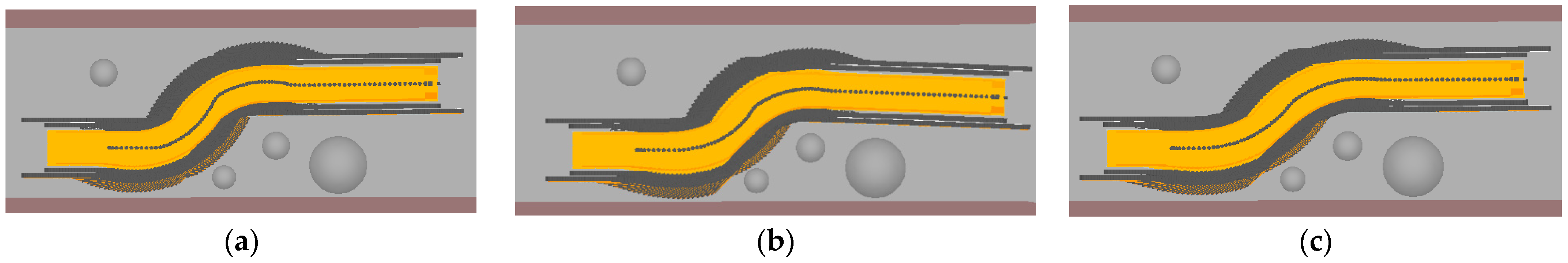
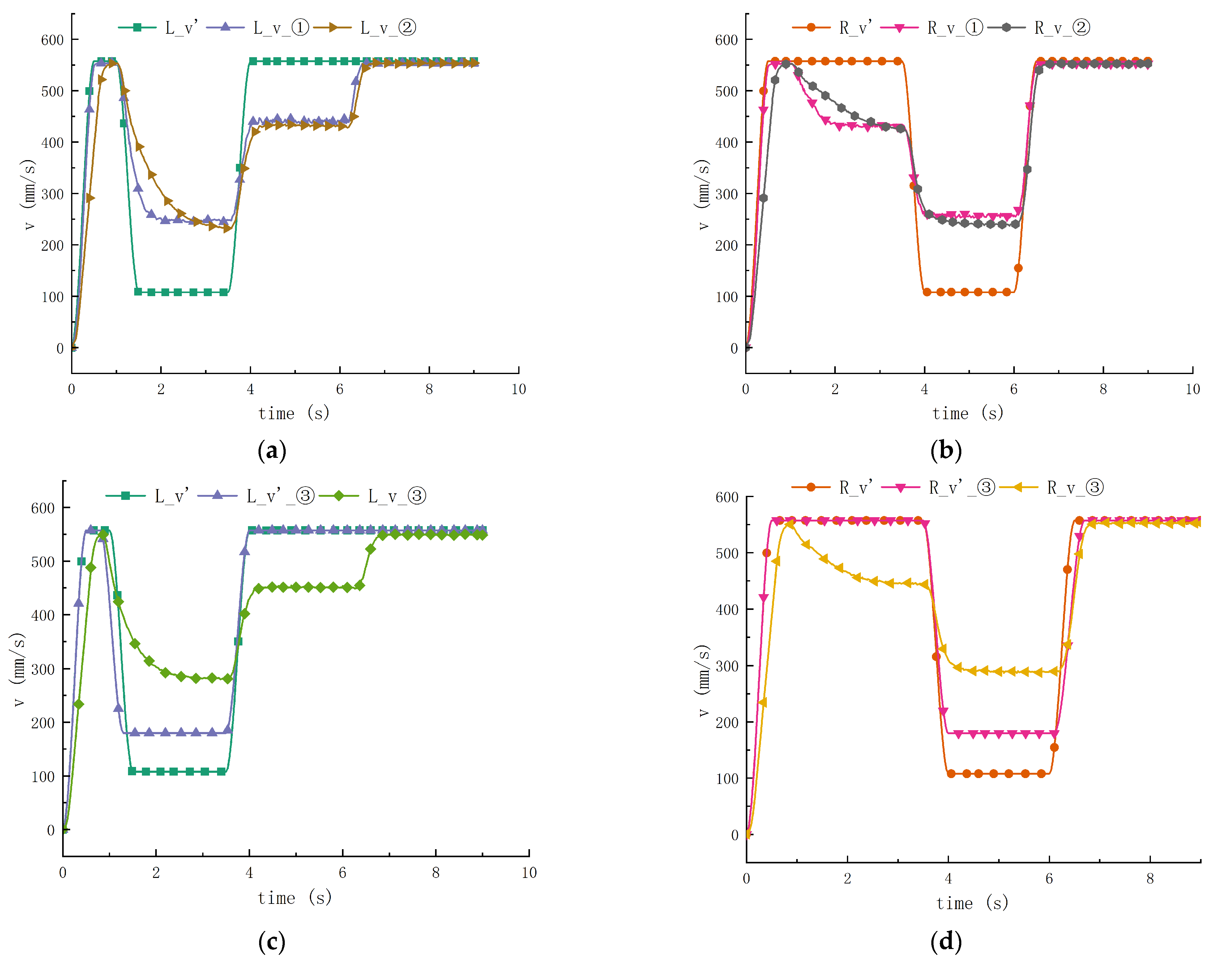
5.3. Differential Steering Simulation Analysis

In the process of differential steering, the robot needs to master the size, direction, and road parameters of obstacles in advance to determine the track driving parameters. Because the robot is driving under different road conditions, although there are the same driving parameters, the steering effect of the robot will be different. When the robot travels on different road surfaces, even with the same driving parameters, the robot’s steering performance varies. For instance, on rough terrain, the robot can achieve obstacle avoidance steering with a smaller turning radius. However, when using the same driving parameters to steer the robot on smoother terrain, the robot requires a larger turning radius, which may lead to collisions with nearby obstacles.

This study defines two types of road surface conditions: one is a rough road surface, and the other is a smooth road surface, each characterized by a different S_coefficient and D_coefficient. Scheme 1 involves the tracked robot using control strategy 1 for obstacle-avoidance on a rough road surface. Scheme 2 involves the tracked robot using control strategy 1 for obstacle avoidance on a smooth road surface. Scheme 3 involves the tracked robot using control strategy 2 for obstacle avoidance on a smooth road surface, as depicted in Figure 13.

The robot adopts the same control strategy for obstacle-avoiding steering movements on different roads, but their trajectories are completely different, as shown in Figure 13a,b. By adjusting the driving parameters of the robot track, the obstacle avoidance steering movement is completed according to the requirements, as shown in Figure 13c.

Table 3. Parameters and results of differential steering.

Scheme		Scheme 1	Scheme 2	Scheme 3
Road properties		rough road surface	smooth road surface	smooth road surface
Control strategy		control strategy 1	control strategy 1	control strategy 2
Contact parameters	S_coefficient	0.3	0.1	0.1
	D_coefficient	0.1	0.05	0.05
Steering radius (mm)	Ra’1	585	585	771
	Ra1	930	967	1220
	Ra’2	585	585	585
	Ra2	978	959	1266

lists the simulation parameters and results for the robot in the ADAMS virtual prototype. where Ra represents the actual steering radius, Ra’ represents the theoretical steering radius, and the numbers 1 and 2 represent the number of steering control strategies. It can be observed that the actual steering radius of the robot is larger than the theoretical steering radius, particularly when the robot is driving on poor roads, and the difference between the theoretical and actual values is larger.

The theoretical and actual velocity curves of the left and right tracks during the steering process of the robot are shown in Figure 14, where R and L represent the right and left tracks, respectively, and V and V′ represent the actual traction speed and theoretical traction speed, respectively. The numbers ①, ②, and ③ represent the serial numbers of the three control schemes. Figure 14a,b show the obstacle avoidance steering motions of the robot using the same control strategy on different roads; however, their velocities are completely different. By adjusting the driving parameters of the robot track, the robot completed the obstacle avoidance steering motion, as required, as shown in Figure 14c,d. Through the simulation analysis of differential steering, it becomes evident that the speed of the robot’s two tracks undergoes minimal change, enabling the robot to adeptly execute obstacle avoidance steering maneuvers with efficiency.

The skid and slip rates always changed during the steering process of the robot, as shown in Figure 15a. Let i represent the skid or slip rate of a track. The part above the zero axis represents the slip rate and the part below the zero axis represents the skid rate. When the robot started, the slip rate decreased with an increase in the robot’s speed, as shown at point A. When the robot turned to the left, the left track skidded and its value was negative. The right track slipped, and its value was positive, as shown at point B. When the robot turned to the right, the left track skidded and its value was positive. The right track slipped, and its values were negative, as shown at point C. Based on the comparative analysis of Figure 15a,b, it is evident that when the robot navigates on a bad road surface, the skid and slip rates of the robot are greater compared to when the robot operates on a good road surface. Through the adjustment of the driving parameters of the two tracks, the robot can effectively execute obstacle avoidance steering maneuvers, leading to a reduction in both the sliding rate and slip rate of the robot, as shown in Figure 15c. The skid and slip rate changes of the robot under different road and control strategies are shown in

Table 4. The skid and slip rate of robot through differential steering.

Point	iR_①	iL_①	iR_②	iL_②	iR_③	iL_③
point A	0.59	0.59	0.66	0.66	0.8	0.8
point B	0.01~0.23	−0.56	0.01~0.24	−0.71~−0.53	0.01~0.2	−0.54~−0.37
point C	−0.56	0.01~0.23	−0.60~−0.54	0.22	−0.42~−0.38	0.19

.

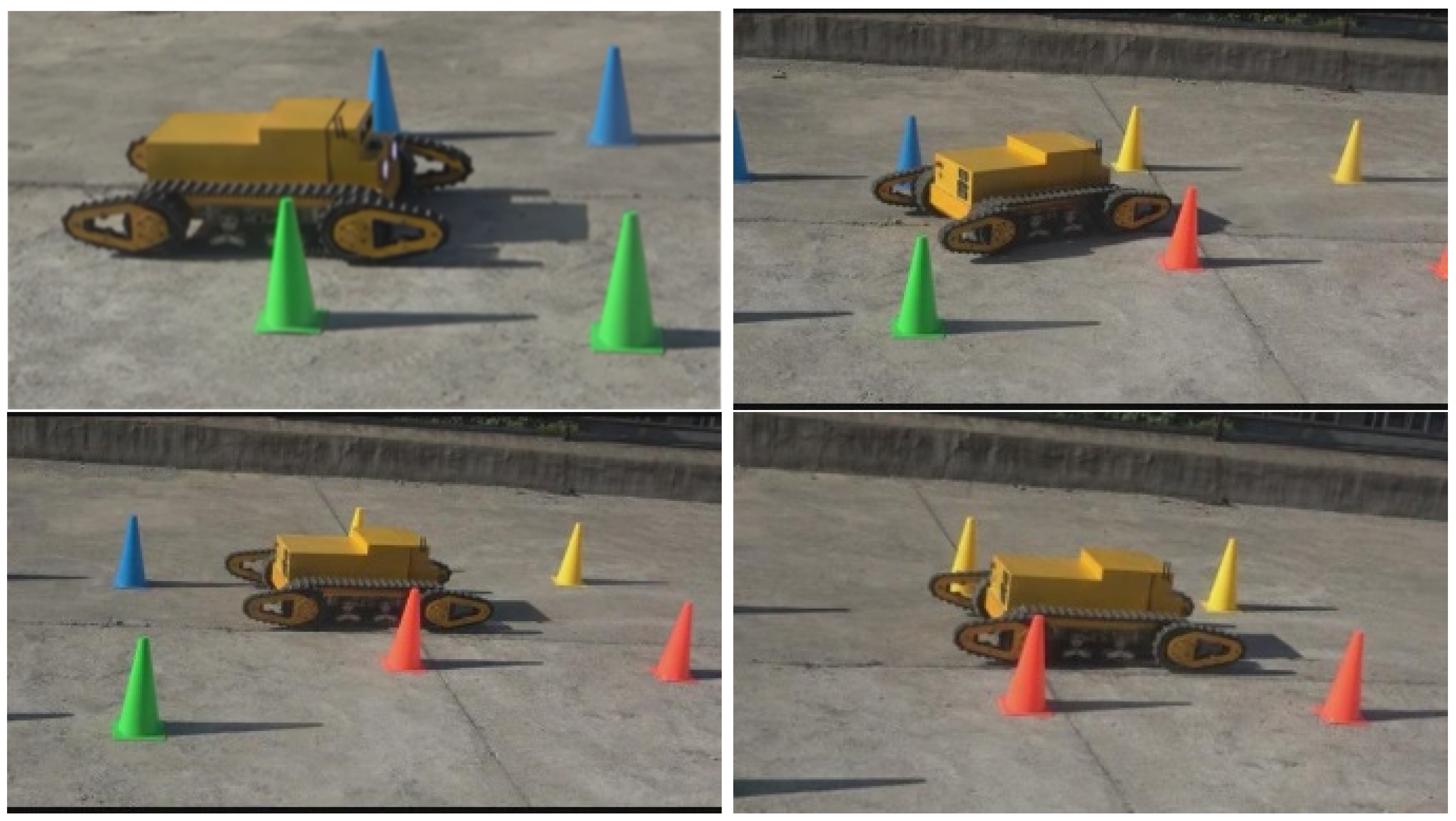
5.4. Test and Analysis of Robot Obstacle Avoidance Steering

In this experiment, the obstacle avoidance steering control performance of the robot was tested by placing obstacles. The robot’s operating space and the layout of obstacles are depicted in Figure 16, where the red line ABOCD represents the robot’s theoretical path, and the red, yellow, green, and blue circles represent the obstacles. The actual obstacle avoidance steering process of the tracked robot is shown in Figure 17. Figure 18 illustrates the comparison between the theoretical and actual paths of the robot’s steering. The reference trajectory is the theoretical driving trajectory of the tracked robot, shown by the red line in Figure 16; the actual trajectory is the actual trajectory of the robot driving on the road, which is calculated by LiDAR and IPC.

From Figure 18, it can be observed that during the testing of the robot’s obstacle avoidance steering performance, despite accounting for the effects of slip and slide between the tracks and the ground, there is still some degree of discrepancy between the theoretical path and the test path. The maximum error occurs during the robot’s steering process, with a maximum deviation of 49.5 mm. At this time, the steering resistance of the robot track is relatively large, which causes the skid and slip rate of the robot to be relatively large, and finally leads to a large deviation in the robot’s driving trajectory.

The testing experiment of the robot’s obstacle avoidance steering illustrates that the tracked robot is capable of executing obstacle avoidance steering movements through various strategies. By taking into account the skidding and slipping characteristics of the robot’s tracks and utilizing information from the surrounding obstacles and road conditions, predetermined driving parameters for the robot’s two tracks enable the tracked robot to proficiently accomplish obstacle avoidance steering. In future work, with the development of more advanced robot obstacle-avoiding steering control algorithms, the steering motion of tracked robots is expected to be further improved.

6. Conclusions

This paper employs obstacle avoidance steering control theory in the context of tracked robots, mitigating the impact of skidding and slipping on their driving control and enhancing the effectiveness of obstacle avoidance steering.

Thia paper analyzed the correlation between the theoretical and practical steering radii and the speed of the two tracks while accounting for the impact of skid and slip. Relationship models were developed linking track speed, driving force, and track turning radius. The research delved into the spatial requirements for robot steering, identifying the maximum and minimum steering radii essential for the robot’s steering maneuvers. A corresponding relationship was established between the robot’s steering angle and the presence of side obstacles. A correction model of the tracked robot was established. Additionally, this paper delved into LiDAR’s detection principle and constructed a robot measurement and control system comprising sensing and signal processing layers, decision control layers, and motion execution control layers. Virtual prototype simulation models for both the tracked robot and obstacles were developed using ADAMS. The simulation experiments encompassed center steering and differential steering, with the finding that employing the differential steering method, based on surrounding obstacle and road surface information, enhances the steering efficiency of tracked robots. This paper concludes by highlighting the use of theoretical guidance to conduct obstacle avoidance steering experiments with the robot, effectively validating the accuracy of the theoretical analysis.

In this paper, an obstacle avoidance steering control strategy based on road parameters and the position of obstacles is proposed, but some errors are admitted. Future research should focus on the online estimation of road parameters and the further development of obstacle avoidance steering control algorithms.

References

1. Mitch, L. Robots Tackle DARPA Underground Challenge. Engineering 2022, 13, 2–4. [Google Scholar]
2. Wang, C.; Wang, D.; Pan, W.; Zhang, H. Output-Based Tracking Control for a Class of Car-Like Mobile Robot Subject to Slipping and Skidding Using Event-Triggered Mechanism. Electronics 2021, 10, 2886. [Google Scholar] [CrossRef]
3. Liu, W.; Luo, X.; Zeng, S.; Zeng, L.; Wen, Z. The Design and Test of the Chassis of a Triangular Crawler-Type Ratooning Rice Harvester. Agriculture 2022, 12, 890. [Google Scholar] [CrossRef]
4. Zhao, J.; Zhang, Z.; Liu, S.; Tao, Y.; Liu, Y. Design and Research of an Articulated Tracked Firefighting Robot. Sensors 2022, 22, 5086. [Google Scholar] [CrossRef] [PubMed]
5. Shafaei, S.M.; Mousazadeh, H. On the power characteristics of an unmanned tracked vehicle for autonomous transportation of agricultural payloads. J. Terramech. 2023, 109, 21–36. [Google Scholar]
6. Kayacan, E.; Young, S.N.; Peschel, J.M.; Chowdhary, G. High-precision control of tracked field robots in the presence of unknown traction coefficients. J. Field Robot. 2018, 35, 1050–1062. [Google Scholar] [CrossRef]
7. Chen, T.; Xu, L.; Ahn, H.S.; Lu, E.; Liu, Y.; Xu, R. Evaluation of headland turning types of adjacent parallel paths for combine harvesters. Biosyst. Eng. 2023, 233, 93–113. [Google Scholar] [CrossRef]
8. Jia, W.; Liu, X.; Zhang, C.; Qiu, M.; Zhang, Y.; Quan, Q.; Sun, H. Research on Steering Stability of High-Speed Tracked Vehicles. Math. Probl. Eng. 2022, 2022, 4850104. [Google Scholar] [CrossRef]
9. Xiong, H.; Chen, Y.; Li, Y.; Zhu, H.; Yu, C.; Zhang, J. Dynamic model-based back-stepping control design for-trajectory tracking of seabed tracked vehicles. J. Mech. Sci. Technol. 2022, 36, 4221–4232. [Google Scholar] [CrossRef]
10. Hu, K.; Cheng, K. Dynamic modelling and stability analysis of the articulated tracked vehicle considering transient track-terrain interaction. J. Mech. Sci. Technol. 2021, 35, 1343–1356. [Google Scholar] [CrossRef]
11. Sabiha, A.D.; Kamel, M.A.; Said, E.; Hussein, W.M. ROS-based trajectory tracking control for autonomous tracked vehicle using optimized backstepping and sliding mode control. Robot. Auton. Syst. 2022, 152, 104058. [Google Scholar] [CrossRef]
12. Fang, Y.; Wang, S.; Cui, D.; Bi, Q.; Yan, C. Multi-body dynamics model of crawler wall-climbing robot. Proc. Inst. Mech. Eng. Part K J. Multi-Body Dyn. 2022, 236, 535–553. [Google Scholar] [CrossRef]
13. Ding, Z.; Wang, Z.; Su, Z.; Tian, L.; Xiong, Y.; Wu, X.; Tang, Z. A New Model to Predict the Slippage Coefficient of Tracked Vehicles During Steering. IEEE Access 2022, 10, 72006–72014. [Google Scholar] [CrossRef]
14. Wu, J.; Wang, G.; Zhao, H.; Sun, K. Study on electromechanical performance of steering of the electric articulated tracked vehicles. J. Mech. Sci. Technol. 2019, 33, 3171–3185. [Google Scholar] [CrossRef]
15. Yang, C.; Yang, G.; Liu, Z.; Chen, H.; Zhao, Y. A method for deducing pressure–sinkage of tracked vehicle in rough terrain considering moisture and sinkage speed. J. Terramech. 2018, 79, 99–113. [Google Scholar] [CrossRef]
16. Kuwahara, H.; Murakami, T. Position control considering slip motion of tracked vehicle using driving force distribution and lateral disturbance suppression. IEEE Access 2022, 10, 20571–20580. [Google Scholar] [CrossRef]
17. Wang, C.; Ma, K.; Yang, L.; Ma, H.; Xue, X.; Tian, H. Simulation and experiment on obstacle-surmounting performance of four swing arms and six tracked robot under unilateral step environment. Trans. Chin. Soc. Agric. Eng. 2018, 34, 46–53. [Google Scholar]
18. Wang, C.; Wang, S.; Ma, H.; Zhang, H.; Xue, X.; Tian, H.; Zhang, L. Research on the Obstacle-Avoidance Steering Control Strategy of Tracked Inspection Robots. Appl. Sci. 2022, 12, 10526. [Google Scholar] [CrossRef]
19. Wong, J.; Senatore, C.; Jayakumar, P.; Iagnemma, K. Predicting mobility performance of a small, lightweight track system using the computer-aided method NTVPM. J. Terramech. 2015, 61, 23–32. [Google Scholar] [CrossRef]
20. Strawa, N.; Ignatyev, D.I.; Zolotas, A.C.; Tsourdos, A. On-Line Learning and Updating Unmanned Tracked Vehicle Dynamics. Electronics 2021, 10, 187. [Google Scholar] [CrossRef]
21. Prado, A.J.; Torres-Torriti, M.; Cheein, F.A. Distributed Tube-Based Nonlinear MPC for Motion Control of Skid-Steer Robots With Terra-Mechanical Constraints. IEEE Robot. Autom. Lett. 2021, 6, 8045–8052. [Google Scholar] [CrossRef]
22. Wong, J.Y.H.; Chiang, C. A general theory for skid steering of tracked vehicles on firm ground. Proc. Inst. Mech. Eng. Part D J. Automob. Eng. 2001, 215, 343–355. [Google Scholar] [CrossRef]
Figure 1. Tracked robot with four swing arms and six tracks.
Applsci 13 11054 g001
Figure 2. Skid and slip analysis of robot track.
Applsci 13 11054 g002
Figure 3. Analysis of tracked robot steering radius.
Applsci 13 11054 g003
Figure 4. Relationship between steering radius and obstacle position.
Applsci 13 11054 g004
Figure 5. Relationship between steering angle and obstacle position: (a) relationship between steering angle and structural parameters of robot; (b) relationship between maximum steering angle of robot and distance of lateral obstacles in Matlab.
Applsci 13 11054 g005
Figure 6. Correction principle of robot position and attitude adjustment.
Applsci 13 11054 g006
Figure 7. Detection principle of LiDAR: (a) the detection range of LiDAR; (b) detection interface of LiDAR.
Applsci 13 11054 g007
Figure 8. Overall framework of inspection robot measurement and control system.
Applsci 13 11054 g008
Figure 9. Obstacle avoidance steering control strategy.
Applsci 13 11054 g009
Figure 10. Constraints between robot components.
Applsci 13 11054 g010
Figure 11. Simulation of center steering: (a) strategy 1: the influence of the position relationship between the robot and the obstacles has not been considered; (b) strategy 2: the influence of the position relationship between the robot and the obstacle has been considered.
Applsci 13 11054 g011
Figure 12. Simulation data of center steering: (a) The theoretical and actual velocity of left track in strategy 1; (b) the theoretical and actual velocity of right track in strategy 1; (c) the theoretical and actual velocity of left track in strategy 2; (d) the theoretical and actual velocity of right track in strategy 2. (e) Skid and slip rate of two tracks in strategy 1; (f) skid and slip rate of two tracks in strategy 2.
Applsci 13 11054 g012aApplsci 13 11054 g012b
Figure 13. Obstacle avoidance steering trajectory of the robot using large-radius steering: (a) Scheme 1; (b) Scheme 2; (c) Scheme 3.
Applsci 13 11054 g013
Figure 14. The velocity curve of differential steering of the robot: (a) the velocity of the left track in Schemes 1 and 2; (b) the velocity of the right track in Schemes 1 and 2; (c) the velocity of the left track in Scheme 3; (d) the velocity of the right track in Scheme 3.
Applsci 13 11054 g014
Figure 15. The skid and slip rates of robot under different road and control strategies: (a) Scheme 1; (b) Scheme 2; (c) Scheme 3.
Applsci 13 11054 g015
Figure 16. Robot trajectory and spatial position of obstacle relationship.
Applsci 13 11054 g016
Figure 17. Three-dimensional view of obstacle avoidance steering tests.
Applsci 13 11054 g017
Figure 18. Error analysis of robot obstacle-avoiding steering trajectory.
Applsci 13 11054 g018