Abstract
Cancer diagnosis and treatment depend on accurate cancer-type prediction. A prediction model can infer significant cancer features (genes). Gene expression is among the most frequently used features in cancer detection. Deep Learning (DL) architectures, which demonstrate cutting-edge performance in many disciplines, are not appropriate for the gene expression data since it contains a few samples with thousands of features. This study presents an approach that applies three feature selection techniques (Lasso, Random Forest, and Chi-Square) on gene expression data obtained from Pan-Cancer Atlas through the TCGA Firehose Data using R statistical software version 4.2.2. We calculated the feature importance of each selection method. Then we calculated the mean of the feature importance to determine the threshold for selecting the most relevant features. We constructed five models with a simple convolutional neural networks (CNNs) architecture, which are trained using the selected features and then selected the winning model. The winning model achieved a precision of 94.11%, a recall of 94.26%, an F1-score of 94.14%, and an accuracy of 96.16% on a test set.
1. Introduction
Cancer is a leading cause of death globally, and it is, the second leading cause of death in the United States after heart disease. In the US, Cancer mortality reached 163.5 per 100,000 persons. Worldwide, 609,820 cancer-related deaths, and more than 1.9 million new cancer diagnoses are anticipated for 2023 [1]. Furthermore, according to data from 2013 to 2015, 38.4% of Americans will receive a cancer diagnosis at some point in their lifespan. Cancer detection and treatment methods have been the subject of extensive research to decrease its negative effects on human health. Cancer prediction places much emphasis on cancer susceptibility, recurrence, and prognosis. A shift toward multi-omics investigations is occurring [2,3], focusing strongly on genomes, transcriptomics, and proteomics. The goal is to give clinicians a more profound understanding of patients’ internal states to make accurate clinical decisions. A comprehensive understanding of the intricacies of the patterns involved in the cancer process is provided by recent improvements made through collaborations between machine learning and gene expression data analysis of cancer [4]. Therefore, gene expression data raises the necessity for cutting-edge machine learning techniques, which increasingly serve as one of the primary motivators for numerous clinical and translational applications.
Recently, a combination of new facilities and technologies has generated vast amounts of cancer data, which hold immense potential for advancing our understanding of cancer. Due to the accessibility of publicly available cancer data over the past ten years, traditional machine learning approaches have been developed [5,6,7,8,9,10]. On the other hand, a set of neural network models with multi-layers called deep learning (DL) excels at the challenge of being trained with large amounts of data. Like traditional machine learning techniques, DL entails two steps: training, which involves estimating the parameters of the network from a specified dataset known as the training set, and testing, which uses a testing set to evaluate the learned network performance. The development of deep learning approaches that have innovative interpretability and high accuracy in predicting the types of cancers was made possible by accumulating whole transcriptome profiling of tumor data. One of these profiling data is the Cancer Genome Atlas (TCGA), a well-known cancer transcriptome profiling database containing the 33 most common types of cancer [11]. Many models based on different DL are created for the detection and classification of cancer. Research that utilized multiple models based on convolutional neural networks (CNNs) built for various input data types was reported by Milad Mostavi et al. in their publication [12]. These models rigorously examine the ability of the convolution kernels. Milad Mostavi et al. assessed the performance of their models in predicting tumor types using the TCGA data, which contains the gene expression of 33 types of cancer. Their models achieved prediction accuracies ranging from 93.9% to 95%. Four Graph CNNs models were suggested and trained by Ricardo Ramirez et al. [13] utilizing the whole TCGA gene expression data sets to classify 33 different cancer types. The models had prediction accuracies from 89.9 to 94.7%. Lyu et al. [14] developed a CNNs model and obtained more than 95% classification accuracy for 33 cancer types retrieved from TCGA. They mapped the gene expression samples into two-dimensional matrices for input. Zexian Zeng et al. [15] presented a CNNs approach for the classification of seven types of cancer retrieved from the TCGA dataset and obtained an overall accuracy of 77.6%. Our group [16] proposed five 1D-CNN-based stacking ensemble approaches for classifying the most malignancies affecting women. The developed model uses RNASeq data obtained from TCGA as an input. The output of these models is integrated using Neural Network (NN), which is then utilized as a meta-model.
Ramroach et al. [17] assessed the application of five different machine learning (random forest, GBM, REFRN, SVM, and KNN) with RNAseq data from 17 cancer types. In a recent study, researchers compared the performance of different machine learning algorithms for cancer research. They split the data into two sets: 75% for training and 25% for testing. Their models were built using the training set, and the testing set was used to evaluate their models performance. The researchers found that ensemble algorithms performed better than the other methods on the entire gene list. Ensemble algorithms are a techniques or algorithm that combines the predictions of multiple models. This can help to enhance the models’ performance by reducing the bias and variance of individual models. At the same time, the clustering and classification models achieved higher performance when features (genes) were reduced to 20 genes. Hong et al. [18] created a multitask model based on deep learning for classifying tissue, disease condition, tissue origin, and neoplastic subtype using the full transcriptome (RNA-seq) datasets peri-neoplastic, neoplastic, and non-neoplastic tissue. Their results indicated that the model achieved 99% accuracy for classifying disease states, an accuracy of 97% for classifying tissue origin, and an accuracy of 92% for subclassification of neoplastic. Khan and Lee [19] proposed a gene transformer deep learning-based model to detect the significant biomarkers across different cancer subtypes. They used gene expression data of 33 tumor types from the TCGA. Their results indicated that their proposed model outperformed the traditional classification models. Zhang et al. [20] developed an explainable deep learning model called Transformer for Gene Expression Modeling (T-GEM) for predicting the cancer types and identifying the type of immune cell using TCGA and ScRNA-Seq data, respectively. Moreover, they used their proposed model to obtain the relevant markers. Their results depicted that their developed model has accuracies of 94.92% and 90.73% for the TCGA and PBMC ScRNA-Seq datasets, respectively. Lkf Cai et al. [21] created a transformer deep learning model called DeePathNet that combines omics data and pathways information. They used the datasets TCGA, CCLE, and ProCan-DepMapSanger. The performance of their proposed model was assessed by classifying cancer types and subtypes, in addition to the prediction of the drug response. Their proposed model outperformed the traditional classifiers by achieving over 95% recall scores for most cancer types.
In this paper, we constructed a CNNs model that classifies 33 cancer types and normal samples using RNA-Seq gene expressions data as inputs. The Illumina HiSeq platform and R software are used to obtain gene expression data from Pan-Cancer Atlas [22] via the RTCGAToolbox package [23,24]. We selected the state run data of 28-01-2016, which is determined using the getFirehoseRunningDates function. Consequently, the getFirehoseData function is used to download the gene expression data. Then, we processed the downloaded data using a normalization technique to the data to ensure that the expression could be inferred properly from the gene expression data and prevent the occurrence of biased expression scores. The normalized data is processed using filtration through the gene-filter package to filter the genes that exhibit low variation across the samples.
2. Materials and Methods
The R/Bioconductor package RTCGA Toolbox package [24] is used to retrieve the Pan-Cancer Atlas RNASeq gene expression data via the TCGA Firehose Data. The obtained data contains 10,456 samples from 33 tumor types with their corresponding normal samples and it has 20,501 genes in total. The gene expression data was log2 transformed using the formula . Thereafter, dataset undergoes normalization and filtration processes, which reduced the number of genes to 15,271. Figure 1 presents the number of sample in each cancer type.
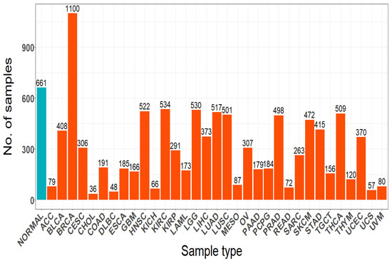
Figure 1.
Total samples number for each cancer type and normal cases.
3. Proposed Approach
Figure 2 depicts the complete framework of our proposed method. First, we divided the entire data into testing and training sets before processing it with feature selection algorithms to prevent data leakage and model overfitting. Then, we applied feature selection procedures to the training set. This way, we will ensure no information is shared between the training and testing sets when applying the features selection algorithm. Suppose feature selection is used to prepare the data, followed by model selection and training on the chosen features. In this case, the model will be given the training set as a whole for making feature selection decisions. This could lead to models that are improved by the chosen features over other tested models appearing to have better results when they have biased results [25]. Three feature selection techniques are used. These techniques are Lasso, Random Forest, and Chi-Square. These feature selection techniques are essential because they can identify the most important features that strongly impact the target variable and remove the less important features. We calculated the feature importance of each selection method. Then we calculated the mean of the feature importance to determine the threshold for selecting the most relevant features, which are then reshaped into 2D-image-like data. The thresholds that we used in this research are µ, 0.5 µ, 2 µ, 4 µ, and 8 µ and they are used to create five classification models. These classification models are trained based on a 10-fold cross-validation approach.
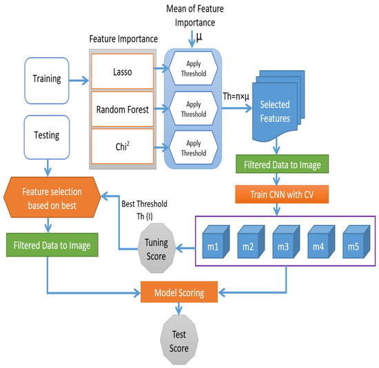
Figure 2.
Overall framework for the proposed method.
Lasso is a regularization technique that enhances the functionality of linear regression models. To achieve this, a penalty that promotes the coefficients of less important characteristics to be zero is added to the loss function [26]. This makes the model easier to understand and more straightforward. Both classification and regression issues can be solved with Lasso. When there are many features, and the target variable is only affected by a small number of features, Lasso performs well. A penalty factor determines the number of features that are maintained. Choosing the penalty factor using cross-validation increases the likelihood that the model will generalize well to new data sets.
If we consider a multinomial response with more than two levels , we can suppose that , where represents the probability of observing ith response. The multinomial LASSO model’s log-likelihood can be expressed as follows [27]:
The aforementioned log-likelihood can be optimized through a penalized approach. Therefore, the regularized log-likelihood in Equation (1) can be represented in more detailed as follow
The target variable can be represented by a matrix, where has a dimension of, and. is a vector that represents the regression parameters, the penalty component of the equation above denoted by , the level of expression for the gene of sample is represented by , and the response value for sample . The penalty of LASSO regression can be achieved by setting in Equation (3).
The reason that LASSO was chosen as the penalty term is that it uses the total actual parameters’ values used in the model, which are constrained to be lower than a predetermined threshold. In statistics, the chi-square test determines if two events are independent [28]. Equation (4) shows the calculation of chi-Square statistics where we can obtain the actual count O and the expected value E from two variables’ data. Chi-Square determines the discrepancy between the anticipated count E and the actual count O. While choosing features. Our goal is to select those that depend heavily on the outcome. The observed count will be relatively close to the expected count if the two features are independent. Hence, the value of the Chi-Square statistics will be smaller. A high Chi-Square statistic indicates that the independence hypothesis is not true. As a result, features with higher Chi-Square statistics will be selected for training the model.
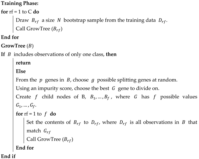
Random Forests (RF) is a learning method based on an ensemble approach that builds many decision trees during training and returns each tree’s mean prediction or mode of the classes [29]. Problems involving classification and regression are both addressed by RF. RF chooses the most crucial features based on the impurity reduction they offer, and the most vital characteristics offer the most significant impurity reduction. The RF algorithm procedure is presented in Algorithm 1 [25].
| Algorithm 1. Random Forests Pseudocode |
 |
| Prediction Phase: |
| To predict a new sample : let the probability assigned by classifier random forest tree. Therefore, the |
4. Performance Score
In this work, we used four metrics to assess our proposed model. These metrics, namely, F1-score, precision, recall, and classification accuracy are frequently used to assess a model’s performance on bioinformatics data. F1- score and accuracy are used to assess the model’s overall performance. In addition, the sensitivity and recognition rate are scored by recall and precision, respectively. The mathematical expressions for these metrics are provided below. The percentage of correctly recognized cancer is the classification accuracy, which is computed as follows:
Recall is a metric used in machine learning to assess a model’s capacity to locate all pertinent instances within a set of data. The ratio of true positives to the total of true positives and false negatives is used to compute it and its equation is as follows:
A classification model’s precision is its capacity to recognize only the relevant data points, which is given by:
A model’s accuracy on a binary classification process is called the F1 score. It is calculated as the mean of recall and precision, where 1 reflects the highest value and 0 reflects the worst value. Precision and recall both contribute the same percentages to the F1 score. The F1 score can be presented as follows:
5. Results and Discussion
Keras Library [30] was used to implement our deep-learning approach. The original dataset contains 15,271 genes (features). As mentioned in the proposed method section, we initially split the entire dataset into testing and training sets. The training data was then used to create our model. We designed a CNN models that is very simple in which we limited the number of convolutional layers to one convolutional layer. That is because Increased CNN model depth does not necessarily improve the performance on bioinformatics data [31], even though deeper models based on CNN have shown great performance in computer vision problems [32]. For problems like the prediction of a cancer type, shallower models are recommended when the samples’ number is quite tiny compared to the number of factors. Such simple models use fewer training resources and prevent overfitting [33]. Based on these two factors, we built a CNN model that adheres to the most often used models in computer vision when the input has a two-dimension format, such as an image. The 2D kernels in this CNN are used to extract local features. The size, number, and stride of the kernel parameters, as well as the total amount of nodes in the fully linked layers, are tuned using the grid search method [34].
We first started by training our designed CNN model using the entire features (genes). The features are reshaped into 2D-image-like data to be appropriate for our designed CNN model. Since the training data has imbalanced classes, we set the class weight parameter to ‘’balanced’’ to automatically adjust the weights based on the class frequencies in the training data. We utilized the cross-validation method with a leave-one-out to assess the correctness of our model. Our training data set was initially divided into ten roughly equal sets. The validation set was represented by the elimination of one set, and the training set was created by pooling the remaining nine sets. We carried out this procedure ten times, substituting one set for the validation set each time. We will have a different validation set each time this way, allowing us to assess the generalizability of our model. We evaluated the model on the test set and the obtained results are shown in Table 1.

Table 1.
Models’ accuracies when using the entire features.
We applied Lasso, Chi-Square, and Random Forest features selection to select the genes that significantly affect the class by calculating their feature importance. To select the most relevant features, we used five thresholds µ, 0.5 µ, 2 µ, 4 µ, and 8 µ on each feature selection method. We used the features selected by these five thresholds to create five CNN classification models each model has the same setting that we adjust for the entire features. The number of features that resulted from the different feature selection methods (Lasso Random Forest, Chi-Square) using the five thresholds together with their corresponding model tuning accuracy based on 10-fold cross validation are presented in Table 2, Table 3 and Table 4.
Table 2.
Models accuracies and the number of features when using Lasso with the different thresholds.
Table 3.
Models accuracies and the number of features when using Random Forest with the different thresholds.
Table 4.
Models accuracies and the number of features when using Chi-Square with the different thresholds.
Table 2, Table 3 and Table 4 show that the model performance on the features that are selected using the features selection method is better compared to it is performance on the entire set of features. As revealed in Table 2, model 4 achieved a tuning accuracy of 97.11% and that makes it as the best model. The features for model 4 are selected using Lasso with feature importance threshold set to 4 µ. The selected threshold produces 597 features that will be used to score the model accuracy on the test data. The best model in Table 3 is model 3, which achieved a tuning accuracy of 96.94%. The features for model 3 are selected using Random Forest. 2 µ is used as feature importance threshold and that produces 1656 features. Table 4 shows that the best model when using Chi-Square as a feature selection method is model 1 with a tuning accuracy of 96.69% at a feature importance threshold equal to 0.5 µ which produces 7137 features. From the above results, it is clear that the best model is the model that resulted from using the Lasso as a features selection method at a feature importance threshold equal to 4 µ. The accuracy obtained from evaluating the best model on the test set is 96.16% with test std: (+/−0.40%). The classification report of the best model for each cancer type and the normal cases is depicted in Table 4. Table 4 shows that the f1-score provides the mean of precision and recall.
The scores given to each class will show how well the classifier classified the data points within that class in relation to all other classes. Table 5 shows that the proposed model has very high identification ability on the classes BRCA, CESC, HNSC, LGG, PCPG, PRAD, SKCM, TGCT, THCA, and UCEC with F1-score ranging between 98% and 99%. In addition, the table shows that the proposed model performed very weak in classifying CHOL class, where only 35 samples from CHOL class were included in the modeling process.
Table 5.
The classification report for each cancer type in addition to the normal cases.
Figure 3 shows the proposed model Confusion matrix on 33 tumor types in addition to the normal samples. By examining the confusion matrix carefully, it is clear that the majority of errors are in the classification of READ, KICH, ESCA, and CHOL. For the READ (Rectum adenocarcinoma or rectal cancer) cancer type, 39% of the samples were misclassified as COAD (colon adenocarcinoma), while 12% of the samples of COAD were misclassified as READ. In the rectal cancer, the tissues of the rectum evolve into cancerous (malignant) cells. The rectum is the last several inches of the large intestine, connecting it to the anus while the colon cancer starts in the colon, which is the longest part of the large intestine. Adeno-matous polyps, which are tiny, noncancerous (benign) cell clusters, are the precursors to both types of cancer and some of these polyps may develop into cancer over time. This misclassification between READ and COAD is observed in the study [13]. Also, Study [14] discovered that the patterns of genetic alterations in rectum and colon tumors were quite comparable. The same goes for the incorrect classification of 29% and 14% of cholangiocarcinoma (CHOL), a kind of liver cancer that develops in the bile duct, into liver hepatocellular carcinoma (LIHC) and lung adenocarcinoma (LUAD) respectively. It’s crucial to remember that CHOL and LIHC are the two most prevalent primary liver malignancies worldwide. The biopotential for liver stem cells to develop into either hepatocytes or cholangiocytes has been accepted as a continuous liver cancer spectrum [35]. Figure 3 also shows that the proposed model is able to classify the eight classes (UVM, UCS, THYM, OV, MESO, LAML, GBM, and DLBC) into their corresponding class. These eight cancers types were classified with 100% accuracy because they have small sample sizes, which is a challenge of many medical data. Since we are aiming for robustness, generalization, and realistic performance on unseen data it’s crucial to take steps to address this issue in our future study because realistic performance is more important than perfect accuracy on the training data.
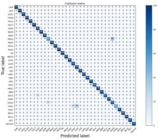
Figure 3.
The proposed model Confusion matrix on 33-tumor type in addition to the normal samples.
Table 6 shows the comparison between our proposed method, Mostavi et al. [12], and Ramirez, Ricardo [13]. Mostavi et al. and Ramirez, Ricardo used the same RNA-Seq gene expression data that we used, which covered 33 different cancer types. With accuracy of (96.16% +/−0.40%), precision of 94.11%, recall of 94.26%, and F-score of 94.14, our suggested technique outperforms these other methods. The precision, recall, and F1-score of the PPI + singleton GCNN model were calculated from their constructed confusion matrix. Also, the recall and F1-score for Mostavi et al. were calculated from their constructed confusion matrix. The calculation was done using the caret package in R via the confusion Matrix function, which retrieves each class’s precision, recall, and F1-score. Then we calculated the average of these scores from the different classes.
Table 6.
Evaluation of proposed approach with existing techniques for classifying cancer types.
The impact of the features selection techniques on the classification accuracy is depicted in Table 7 below. Despite the fact that our method was applied to 33 cancer kinds, the genetic algorithm features selection obtained an accuracy of 90% when employed with the k-nearest neighbors (KNN) algorithm, which is lower than our attained accuracy. In contrast, the work that used a genetic algorithm with a KNN classifier is applied to 31 cancer types. The Table also shows Garcia-Diaz et al. [38] scored an accuracy of 98.81%. Although the accuracy achieved by Garcia-Diaz et al. is greater than our model, the authors applied their methods to only five cancer types.
Table 7.
A comparison with recent methods of features selection.
6. Analysis of the Protein-Protein Association Network
Identifying protein-protein interactions (PPIs) is highly significant when verifying gene selection in the context of various biological and biomedical research areas because it places selected genes in a functional and biological context. It helps to confirm the relevance of chosen genes in various biological processes. To construct the PPI, we obtained the intersection of the lists of the genes that are obtained by each of the three feature selection methods (Chi square (7137 genes), RF (1656 genes), and LASSO (597 genes). The intersection yielded 301 genes that are commonly significantly associated with the 33 cancer types. The STRING database and the Cytoscape tool were used to build the protein-protein interaction network (PPI). Figure 4 illustrates the developed PPI network. The eccentricity of a node in a biological network is scored by how easily all other proteins in the network may functionally reach that node.
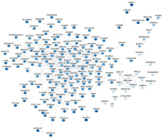
Figure 4.
PPI – the dark blue indicates high eccentricity, while light blue indicates low eccentricity.
To obtain the most significant genes and get a clear understanding of the top genes that can identify the cancer type we constructed the network for genes that have high degree (number of edges) using the two methods maximum neighborhood component (MCN) and maximal clique centrality (MCC). We used CytoHubba plugin by setting its parameters to the default values to select the to 10 genes from the PPI network. The 10 genes that are obtained by the two aforementioned methods are depicted in Figure 5.
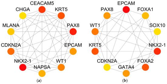
Figure 5.
The Top 10 genes that are obtained using maximum neighborhood component (MCN) and maximal clique centrality (MCC). (a) Top 10 hub genes using MCC method. (b) Top 10 hub genes using MNC method.
The six common hub genes can be obtained by taking the intersection of the MCC and MNC methods. These six genes are PAX8, KRT5, CDKN2A, EPCAM, WT1, NKX2-1. To show the effectiveness of our features selection method we further studied the impact of these top 6 selected genes in cancer using previous studies. I.e. Di Palma et al. [39] show that the organogenesis of the thyroid gland, kidney, neurological system, and Müllerian system depends on PAX8. Also, they demonstrate in earlier research that PAX8 is essential for thyroid differentiated epithelial cells’ cell cycle progression and survival [40,41]. The tumors of gliomas, well-differentiated pancreatic neuroendocrine malignancies, renal, thyroid, ovarian, Wilms, and other cancers have all exhibited PAX8 positivity [42]. In addition, PAX8 is a helpful marker for primary or metastatic neoplasms diagnosis because it is not expressed in primary tumors of the breast, lung, or mesothelium [43]. PAX8 was found to be a survival gene important for ovarian cancer cells’ capacity to proliferate in the OC scenario by the Cancer Genome Atlas (TGCA) Project [44].
In general, PAX8 belongs to a group of lineage-survival genes that are critical for the growth of cancer cells as well as the normal development of specific organs [45]. Regarding KRT5, Ricciardelli et al. [46] found that serous ovarian carcinomas had higher than average KRT5 and KRT6 mRNA expression, which enhanced the likelihood of a disease relapse. Mohtar, M. Aiman [47] show that the basolateral membrane of healthy epithelial cells expresses EpCAM at basal levels. However, solid epithelial malignancies and stem cells produce EpCAM at higher levels. Additionally, circulating tumor cells and disseminated tumor cells also include EpCAM.
The adhesion molecule for epithelial cells EpCAM, which is overexpressed on malignant cells from a range of different tumor types, is only produced by a small percentage of normal epithelia, as demonstrated by Mrich, Sannia, and colleagues [48]. This overexpression is significantly more pronounced in the so-called tumor-initiating cells (TICs) of numerous carcinomas. Chen et al. [49] show that CDKN2A encodes the INK4 family member multiple tumor suppressor 1 (MTS1), which. In comparison to normal tissue, CDKN2A has high levels of expression in tumor tissue, which is indicative of a patient’s prognosis. They concentrated on assessing CDKN2A expression in 33 malignancies, patient prognosis, tumor immunity roles, and clinical characteristics. The amount of CDKN2A expression was highly correlated with the tumor mutation burden (TMB) in 10 tumors, and the same tumors showed a significant correlation between CDKN2A expression and MSI (microsatellite instability). There may be a connection between CDKN2A expression and tumor immunity, as evidenced by the correlation between CDKN2A expression and infiltrating lymphocyte (TIL) levels in 22 pancancers. Chen et al. conducted enrichment analysis, and they found that CDKN2A expression was linked to several malignancies’ control of the autophagy route, olfactory transduction pathways, processing, and dissemination of the antigen and pathways for natural killer cell-mediated cytotoxicity. CDKN2A is also known as cyclin-dependent kinase inhibitor 2A and it plays a vital role in regulating the cell cycle, and its relevance in cancer is significant. It encodes two major protein products (p16INK4a and p14ARF). These proteins are applied in controlling the progression of the cell cycle, preventing uncontrolled cell division, and maintaining genomic stability.
The WT1 gene encodes the crucial transcription factor for normal cellular growth and cell survival, according to Yang, L. et al. [50]. A tumor suppressor gene called WT1 has mutations that have been associated to kidney cancer development and urogenital disease. It was first identified as the causal gene in an autosomal-recessive syndrome. Non-small cell lung cancer (NSCLC), particularly lung adenocarcinoma (ADK), has enhanced expression of NKX2-1, which is an essential molecule in lung development, according to Moisés et al. [51]. In addition, the authors of [52,53] found and evidence suggests that NKX2-1 and TTF-1 play opposing roles in the initiation and progression of lung cancer. These findings may also apply to thyroid tumors and hematological malignancies.
7. Conclusions
In this study, using RNA-Seq gene expression data, we built a deep-learning model to categorize different cancer kinds. To choose the best traits that can be utilized to identify different cancer kinds, we used three different feature selection techniques. For each feature selection method, we calculated the feature’s importance that rate input features according to how well they are able to predict a given target variable. Based on the importance of the features, we devised different thresholds for extracting the best features and then trained five CNN models based on a ten-fold cross-validation approach. For each feature selection approach, we select the most accurate model, and then we select the highest validation accuracy model. The winning model performs well on the test set, with accuracy.
Author Contributions
Data curation, S.N.A.; formal analysis, M.K.E. and M.E.; investigation, M.M, A.M.M. and M.A.; supervision, E.H.; writing—original draft, M.K.E. and M.E.; writing—review and editing, S.N.A., M.M. and A.M.M. All authors have read and agreed to the published version of the manuscript.
Funding
This research was funded by the DEANSHIP OF SCIENTIFIC RESEARCH–JOUF UNIVERSITY, grant number DSR2022-RG-0104.
Institutional Review Board Statement
Not applicable.
Informed Consent Statement
Not applicable.
Data Availability Statement
Furnished on request.
Acknowledgments
The authors acknowledge the Deanship of Scientific research at Jouf University.
Conflicts of Interest
The authors declare no conflict of interest.
References
- Siegel, R.L.; Siegel, R.L.; Miller, K.; Fuchs, H.; Jemal, A. Cancer statistics. CA A Cancer J. Clin. 2022, 72, 7–33. [Google Scholar] [CrossRef] [PubMed]
- Bersanelli, M.; Mosca, E.; Remondini, D.; Giampieri, E.; Sala, C.; Castellani, G.; Milanesi, L. Methods for the integration of multi-omics data: Mathematical aspects. BMC Bioinform. 2016, 17, 167–177. [Google Scholar] [CrossRef]
- Kim, M.; Tagkopoulos, I. Data integration and predictive modeling methods for multi-omics datasets. Mol. Omics 2018, 14, 8–25. [Google Scholar] [CrossRef] [PubMed]
- De Anda-Jáuregui, G.; Hernández-Lemus, E. Computational oncology in the multi-omics era: State of the art. Front. Oncol. 2020, 10, 1–21. [Google Scholar] [CrossRef] [PubMed]
- Kourou, K.; Exarchos, T.P.; Exarchos, K.P.; Karamouzis, M.V.; Fotiadis, D.I. Machine learning applications in cancer prognosis and prediction. Comput. Struct. Biotechnol. J. 2015, 13, 8–17. [Google Scholar] [CrossRef]
- Statnikov, A.; Wang, L.; Aliferis, C.F. A comprehensive comparison of random forests and support vector machines for microarray-based cancer classification. BMC Bioinform. 2008, 9, 1–10. [Google Scholar] [CrossRef]
- Cruz, J.A.; Wishart, D.S. Applications of machine learning in cancer prediction and prognosis. Cancer Inform. 2006, 2, 117693510600200030. [Google Scholar] [CrossRef]
- Liu, J.J.; Cutler, G.; Li, W.; Pan, Z.; Peng, S.; Hoey, T.; Chen, L.; Ling, X.B. Multiclass cancer classification and biomarker discovery using GA-based algorithms. Bioinformatics 2005, 21, 2691–2697. [Google Scholar] [CrossRef]
- Li, Y.; Kang, K.; Krahn, J.; Crouwater, N.; Lee, K.; Umbach, D.; Li, L. A comprehensive genomic pan-cancer classification using The Cancer Genome Atlas gene expression data. BMC Genom. 2017, 18, 508. [Google Scholar] [CrossRef]
- Holzinger, A.; Kieseberg, P.; Weippl, E.; Tjoa, A.M. Current advances, trends and challenges of machine learning and knowledge extraction: From machine learning to explainable AI. In Proceedings of the Machine Learning and Knowledge Extraction: Second IFIP TC 5, TC 8/WG 8.4, 8.9, TC 12/WG 12.9 International Cross-Domain Conference, CD-MAKE 2018, Hamburg, Germany, 27–30 August 2018; Springer: Berlin/Heidelberg, Germany, 2018. [Google Scholar]
- Grossman, R.L.; Health, A.; Ferretti, V.; Varmus, H.; Lowy, D.; Kibbe, W. Toward a shared vision for cancer genomic data. N. Engl. J. Med. 2016, 375, 1109–1112. [Google Scholar] [CrossRef]
- Mostavi, M.; Chiu, Y.; Huang, Y.; Chen, Y. Convolutional neural network models for cancer type prediction based on gene expression. BMC Med. Genom. 2020, 13, 44. [Google Scholar] [CrossRef] [PubMed]
- Ramirez, R.; Chiu, Y.-C.; Hererra, A.; Mostavi, M.; Ramirez, J.; Chen, Y.; Huang, Y.; Jin, Y.-F. Classification of Cancer Types Using Graph Convolutional Neural Networks. Front. Phys. 2020, 8, 203. [Google Scholar] [CrossRef] [PubMed]
- Lyu, B.; Haque, A. Deep learning based tumor type classification using gene expression data. In Proceedings of the 2018 ACM International Conference on Bioinformatics, Computational Biology, and Health Informatics, Washington, DC, USA, 29 August 2018. [Google Scholar]
- Zeng, Z.; Mao, C.; Vo, A.; Li, X.; Nugent, J.; Khan, S.; Clare, S.; Luo, Y. Deep learning for cancer type classification and driver gene identification. BMC Bioinform. 2021, 22, 491. [Google Scholar] [CrossRef] [PubMed]
- Mohammed, M.; Mwambi, H.; Mboya, I.B.; Elbashir, M.K.; Omolo, B. A stacking ensemble deep learning approach to cancer type classification based on TCGA data. Sci. Rep. 2021, 11, 15626. [Google Scholar] [CrossRef] [PubMed]
- Ramroach, S.; John, M.; Joshi, A. The efficacy of various machine learning models for multi-class classification of rna-seq expression data. In Proceedings of the Intelligent Computing: Proceedings of the 2019 Computing Conference, 23 June 2019; Springer: London, UK, 2019; Volume 1. [Google Scholar]
- Hong, J.; Hachem, L.D.; Fehlings, M.G. A deep learning model to classify neoplastic state and tissue origin from transcriptomic data. Sci. Rep. 2022, 12, 9669. [Google Scholar] [CrossRef] [PubMed]
- Khan, A.; Lee, B. Gene transformer: Transformers for the gene expression-based classification of lung cancer subtypes. arXiv 2021, arXiv:2108.11833. [Google Scholar]
- Zhang, T.-H.; Hasib, M.M.; Chiu, Y.; Han, Z.; Jin, Y.; Flores, M.; Chen, Y.; Huang, Y. Transformer for Gene Expression Modeling (T-GEM): An Interpretable Deep Learning Model for Gene Expression-Based Phenotype Predictions. Cancers 2022, 14, 4763. [Google Scholar] [CrossRef]
- Cai, Z.; Poulos, R.; Aref, A.; Robinson, P.; Reddel, R.; Zhong, Q. Transformer-based deep learning integrates multi-omic data with cancer pathways. bioRxiv 2022. [Google Scholar] [CrossRef]
- Weinstein, J.; Collisson, E.; Mills, G.; Shaw, K.; Ozenberger, B.; Ellrott, K.; Shmulevich, L.; Sander, C.; Stuart, J. The cancer genome atlas pan-cancer analysis project. Nat. Genet. 2013, 45, 1113–1120. [Google Scholar] [CrossRef]
- Colaprico, A.; Silva, T.C.; Olsen, C.; Garofano, L.; Cava, C.; Garolini, D.; Sabedot, T.S.; Malta, T.M.; Pagnotta, S.M.; Castiglioni, I.; et al. TCGAbiolinks: An R/Bioconductor package for integrative analysis of TCGA data. Nucleic Acids Res. 2016, 44, e71. [Google Scholar] [CrossRef]
- Samur, M.K. RTCGAToolbox: A New Tool for Exporting TCGA Firehose Data. PLoS ONE 2014, 9, e106397. [Google Scholar] [CrossRef]
- Hastie, T.; Tibshirani, R.; Friedman, J. The elements of statistical learning: Data mining, inference, and prediction. In Data Mining, Inference, and Prediction, 2nd ed.; Springer: New York, NY, USA, 2009. [Google Scholar] [CrossRef]
- Tibshirani, R. Regression shrinkage and selection via the lasso. J. R. Stat. Soc. Ser. B Methodol. 1996, 58, 267–288. [Google Scholar] [CrossRef]
- Friedman, J.; Hastie, T.; Tibshirani, R. Regularization paths for generalized linear models via coordinate descent. J. Stat. Softw. 2010, 33, 1–22. [Google Scholar] [CrossRef] [PubMed]
- Plackett, R.L. Karl Pearson and the chi-squared test. Int. Stat. Rev. Rev. Int. De Stat. 1983, 51, 59–72. [Google Scholar] [CrossRef]
- Breiman, L. Random forests. Mach. Learn. 2001, 45, 5–32. [Google Scholar] [CrossRef]
- Keras, C.F. GitHub. Available online: https://github.com/keras-team/keras (accessed on 15 July 2023).
- Min, S.; Lee, B.; Yoon, S. Deep learning in bioinformatics. Brief. Bioinform. 2017, 18, 851–869. [Google Scholar] [CrossRef]
- LeCun, Y.; Bengio, Y.; Hinton, G. Deep learning. Nature 2015, 521, 436–444. [Google Scholar] [CrossRef] [PubMed]
- Ioffe, S.; Szegedy, C. Batch normalization: Accelerating deep network training by reducing internal covariate shift. In Proceedings of the International Conference on Machine Learning, Lille, France, 6 July 2015; pp. 448–456. [Google Scholar]
- Pedregosa, F.; Varoquaux, G.; Gramfort, A.; Michel, V.; Thirion, B. Scikit-learn: Machine learning in Python. J. Mach. Learn. Res. 2011, 12, 2825–2830. [Google Scholar]
- Kang, X.; Bai, L.; Xiaoguang, Q.I.; Wang, J. Screening and identification of key genes between liver hepatocellular carcinoma (LIHC) and cholangiocarcinoma (CHOL) by bioinformatic analysis. Medicine 2020, 99, e23563. [Google Scholar] [CrossRef]
- De Guia, J.M.; Devaraj, M.; Leung, C.K. DeepGx: Deep learning using gene expression for cancer classification. In Proceedings of the 2019 IEEE/ACM International Conference on Advances in Social Networks Analysis and Mining, Vancouver, BC, Canada, 27 August 2019; Available online: https://doi.ieeecomputersociety.org/10.1145/3341161.3343516 (accessed on 17 August 2023).
- Khalifa, N.E.; Taha, M.H.; Ezzat, D.; Slowik, A. Artificial intelligence technique for gene expression by tumor RNA-Seq data: A novel optimized deep learning approach. IEEE Access 2020, 8, 22874–22883. [Google Scholar] [CrossRef]
- Garcia-Diaz, P.; Berriel, I.; Rojas, J.; Pascual, A. Unsupervised feature selection algorithm for multiclass cancer classification of gene expression RNA-Seq data. Genomics 2020, 112, 1916–1925. [Google Scholar] [CrossRef]
- Di Palma, T.; Zannini, M. PAX8 as a potential target for ovarian cancer: What we know so far. OncoTargets Ther. 2022, 15, 1273–1280. [Google Scholar] [CrossRef]
- Bouchard, M.; Souabni, A.; Mandler, M.; Neubuser, A.; Busslinger, M. Nephric lineage specification by Pax2 and Pax8. Genes Dev. 2002, 16, 2958–2970. [Google Scholar] [CrossRef]
- Plachov, D.; Chowdhury, K.; Walther, C.; Simon, D.; Guenet, J.L.; Gruss, P. Pax8, a murine paired box gene expressed in the developing excretory system and thyroid gland. Development 1990, 110, 643–651. [Google Scholar] [CrossRef]
- Di Palma, T.; Filippone, M.G.; Pierantoni, G.M.; Fusco, A.; Soddu, S.; Zannini, M. Pax8 has a critical role in epithelial cell survival and proliferation. Cell Death Dis. 2013, 4, e729. [Google Scholar] [CrossRef]
- Hardy, L.R.; Salvi, A.; Burdette, J.E. UnPAXing the Divergent Roles of PAX2 and PAX8 in High-Grade Serous Ovarian Cancer. Cancers 2018, 10, 262. [Google Scholar] [CrossRef]
- Ye, J.; Hameed, O.; Findeis-Hosey, J.J.; Fan, L.; McMahon, L.A.; Yang, Q.; Wang, H.L.; Xu, H. Diagnostic utility of PAX8, TTF-1 and napsin A for discriminating metastatic carcinoma from primary adenocarcinoma of the lung. Biotech. Histochem. 2012, 87, 30–34. [Google Scholar] [CrossRef]
- Cheung, H.W.; Cowley, G.S.; Weir, B.A.; Boehm, J.S.; Rusin, S.; Scott, J.A.; East, A.; Ali, L.D.; Lizotte, P.H.; Wong, T.C.; et al. Systematic investigation of genetic vulnerabilities across cancer cell lines reveals lineage-specific dependencies in ovarian cancer. Proc. Natl. Acad. Sci. USA 2011, 108, 12372–12377. [Google Scholar] [CrossRef]
- Ricciardelli, C.; Lokman, N.; Pyragius, C.; Ween, M.; Macpherson, A.; Ruszkiewicz, A.; Hoffmann, P.; Oehler, M. Keratin 5 overexpression is associated with serous ovarian cancer recurrence and chemotherapy resistance. Oncotarget 2017, 8, 17819–17832. [Google Scholar] [CrossRef]
- Mohtar, A.; Syafruddin, S.; Nasir, S.; Low, T. Revisiting the roles of pro-metastatic EpCAM in cancer. Biomolecules 2020, 10, 255. [Google Scholar] [CrossRef]
- Imrich, S.; Hachmeister, M.; Gires, O. EpCAM and its potential role in tumor-initiating cells. Cell Adhes. Migr. 2012, 6, 30–38. [Google Scholar] [CrossRef]
- Chen, Z.; Guo, Y.; Zhao, D.; Zou, Q.; Yu, F.; Zhang, L.; Xu, L. Comprehensive analysis revealed that CDKN2A is a biomarker for immune infiltrates in multiple cancers. Front. Cell Dev. Biol. 2021, 9, 808208. [Google Scholar] [CrossRef]
- Yang, L.; Han, Y.; Saiz, F.; Minden, M. A tumor suppressor and oncogene: The WT1 story. Leukemia 2007, 21, 868–876. [Google Scholar] [CrossRef]
- Moisés, J.; Navarro, A.; Santasusagna, S.; Viñolas, N.; Molins, L.; Ramirez, J.; Osorio, J.; Saco, A.; Castellano, J.J.; Muñoz, C.; et al. NKX2–1 expression as a prognostic marker in early-stage non-small-cell lung cancer. BMC Pulm. Med. 2017, 17, 197. [Google Scholar] [CrossRef]
- Yamaguchi, T.; Hosono, Y.; Yanagisawa, K.; Takahashi, T. NKX2-1/TTF-1: An enigmatic oncogene that functions as a double-edged sword for cancer cell survival and progression. Cancer Cell 2013, 23, 718–723. [Google Scholar] [CrossRef]
- The Cancer Genome Atlas (TCGA) Research Network. Comprehensive molecular characterization of human colon and rectal cancer. Nature 2012, 487, 330–337. [Google Scholar] [CrossRef]
Disclaimer/Publisher’s Note: The statements, opinions and data contained in all publications are solely those of the individual author(s) and contributor(s) and not of MDPI and/or the editor(s). MDPI and/or the editor(s) disclaim responsibility for any injury to people or property resulting from any ideas, methods, instructions or products referred to in the content. |
© 2023 by the authors. Licensee MDPI, Basel, Switzerland. This article is an open access article distributed under the terms and conditions of the Creative Commons Attribution (CC BY) license (https://creativecommons.org/licenses/by/4.0/).