Abstract
We developed an improved depth of extreme point (DEXP) method, characterized as an effective and rapid imaging method that can estimate the depth and distribution of a source quickly. Its main purpose is to solve various challenges. The automatic calculation aspect of the traditional method is often limited; namely, there is a problem with achieving automatic and reliable processing when the observed surface presents undulating topography, and this problem cannot be ignored. Therefore, we propose the addition of the constant method and the hypothetical observed surface method to achieve improvements in the traditional method. Firstly, we test the improved method on the synthetic models to demonstrate its notable advantage: the achievement of a fully automatic calculation without requiring any other additional information such as structural index (SI) values and threshold values. Meanwhile, we also demonstrate its ability and reliability to handle undulating topography with acceptable accuracy for imaging results. Furthermore, we verify the robustness of the improved method by applying it to real gravity data from the potash salt deposit in the Sakhon Nakhon basin, Laos. In this case, the improved DEXP method effectively identified the location of the potash deposit. Moreover, combined with the optimal edge detection method, gravity prospecting for potash salt deposits exhibited significant advantages.
1. Introduction
The rapid imaging method aims at estimating source distribution, including depth, structural index, and density (or susceptibility). It is characterized by a simple algorithm, fast inversion processing, and stable results. One of its significant advantages is that it does not require prior information or iteration, making it a convenient and efficient approach. Several general rapid imaging methods have been developed, including the correlation (probability) method [1,2,3,4,5,6,7], the migration method [8], the DEXP method [9,10,11], the continuous wavelet transform method [12,13,14,15,16,17,18,19], and others. These imaging techniques have proven to be highly effective, particularly for isolated, compact, and depth-limited sources, which make them valuable tools in the field of source distribution estimation.
The depth from extreme points (DEXP) method, initially introduced by Fedi [9], is used to estimate the depth and structural index of potential field sources and generate images of the source distribution [20]. This method involves scaling the potential field, or its partial derivatives, with a specific power law whose exponent is related to the structural index, a quantity related to source geometry. This method has been successfully applied to gravity, magnetic, and self-potential data, providing rapid imaging of the corresponding source distributions [21,22,23] and achieving satisfactory results.
The scale function plays an important role in the DEXP method, and the construction of the scale function depends on the structure index (SI) value; however, the empirical choice of the SI limits the automatic processing capabilities of the methods. To address the limitation, a variety of papers have discussed the solution for automatically selecting the SI. Cellla and Fedi (2009) [24] proposed using the reciprocal of the depth, “q = 1/z”, to obtain the SI, but this method was found to be significantly disturbed in complex multi-source situations, and its reliability depended on judgments made based on rich experience. Fedi et al. (2013) [23] suggested estimating the buried depth using the maximum SI; the result demonstrated satisfactory stability and anti-noise ability. Abbas and Fedi (2014) [25] improved the local wavenumber method with the DEXP method, and it estimated the center depth without the need to offer a presupposed or empirical SI value. Abbas and Fedi (2014) [25] also proposed building the ratio of different-order derivatives, which solved the pre-SI requirement and simplified the algorithm. The potential problem of having a zero denominator in this calculation process was addressed by setting the threshold empirically.
It is evident that much of the research on the DEXP method has primarily focused on determining the appropriate value for the structural index (SI). Two main solutions have been proposed to address the issue: one involves specifying the SI based on experience, while the other replaces the SI with the ratio of different-order derivatives. However, the former approach, relying on experience to determine the SI value, is limited because it requires manual intervention and cannot be easily automated. This limitation hinders the ability of the algorithm to process data automatically. The latter approach, which replaces the SI with the ratio of different-order derivatives, achieves an automatic judgment of the SI satisfactorily. However, a potential issue arises when the denominator of the ratio becomes zero, which can significantly affect the imaging results. To mitigate this problem, a threshold method has been used. Although less than satisfactory, this threshold introduces a new interference factor known as the “trapezoid line”.
Furthermore, when applying it to real data, we observed that the influence of topography cannot be ignored. The surface-to-plane method has been widely used to address this issue. The surface-to-plane method is a commonly used data processing technique in gravity and magnetic exploration for handling the complexity of subsurface media. Its fundamental idea is to transform the actual observed data into the responses of an equivalent layered model and then adjust the parameters of the equivalent layers to achieve the best possible fit between the mode response and the observed data. The method includes techniques such as the variable separation method [26,27,28], the boundary integral method [29,30], the equivalent source method [31,32,33], the Taylor series method [34,35,36], the iterative method [37,38], etc. However, the existing surface-to-plane methods have certain limitations. (1) The effectiveness of these algorisms depends heavily on the specific application condition, such as the location of the source and the terrain, the continuity and smoothness of the terrain, the intensity of undulations, and the number of calculated data points, which is relative to the cost of time. These limited conditions can reduce the versatility and automaticity of the methods. (2) In the geophysics inversion, the more complex the processing, the more noise and errors may be introduced into the calculation; therefore, simpler processes tend to contribute more to the original signal and provide more effective information.
In conclusion, considering the desire for flexibility and reliable imaging results, we believe that two aspects of the DEXP method need to be improved. Firstly, automatic calculation should be enhanced, eliminating the need to manually set the structural index (SI) or threshold values. Secondly, the method should be able to handle undulating terrain data directly, without requiring additional processing steps. Therefore, this paper proposes an improved DEXP method. The main objectives of this method are to eliminate the need for manual intervention in setting the SI or threshold values, meanwhile ensuring stability in the imaging results by avoiding singularity or trapezoid lines and enabling direct application to the undulating terrain data. To validate the effectiveness and reliability of the proposed method, we test the method using both synthetic data and real data from a potash salt deposit.
2. Methodology
In this section, it will begin by introducing the theoretical background of the automatic DEXP method [25]. Subsequently, we will present the comprehensive details of our proposed improved DEXP method proposed in this paper. This enhanced approach offers two significant advantages: firstly, it effectively solves the issue of singularity or trapezoid lines encountered in the traditional DEXP method, and secondly, it successfully mitigates the effect of undulating terrain. The core of the improved DEXP method is based on two key techniques, the adding constant method and the hypothetical observed surface method. The details are as follows:
2.1. Theory of the Automatic DEXP Mehod
Fedi et al. [9] proposed the basic formation stated in Equation (1):
The extreme point of represents the center depth of the source being investigated, and N is the SI value, which is a parameter that varies depending on the type of geological body under consideration. Additionally, the order of vertical derivatives of the field is denoted by n. Furthermore, Abbas et al. [21] proposed the construction of a scale function using two different-order vertical derivatives of the homogenous field, denoted as . This allows for and , where respects the order of derivation and respects the order of derivation. The scaling function, denoted as is expressed by Equation (2):
So, the general form of DEXP is defined as Equation (3):
In the DEXP method, the exponent is a known value that allows for the automatic estimation of the depth to the source. In this estimation process, the structure index (SI) is not required. However, there is a possibility of encountering division by zero or by a very small number, which can affect the numerical estimation. Thus, Abbas et al. [25] proposed a method that involves checking the value of the denominator of using a small amount represented by . This value is taken as a fraction of the maximum of at the current depth level. The equation representing this method is shown in Equation (4):
While , so
2.2. Theory of the Improved DEXP Method
2.2.1. Basic Equation
There are some inherent challenges existing in the application of the automatic DEXP method, including: (a) The selection of is subjective and empirical, which limits the fully automatic process. (b) The value of chosen using the automatic DEXP method is a constant. It can guarantee a satisfactory result for the single model; however, based on the experiment results of the combined models, the reliability of the imaging result obviously decreases.
This paper proposes an improved DEXP method, which targets three specific problems: (a) the best method to choose a stable threshold value is still unclear and un-automatic absolutely, (b) the constant threshold value that is chosen empirically cannot satisfy the combined models’ inversion because different models are characterized by different optimal threshold values, (c) the application of this method to achieve reliable and automatic DEXP imaging when the observed surface exhibits undulating terrain is limited.
The proposed improvements in this paper aim to provide solutions to these challenges by introducing the adding constant method and hypothetical observed surface method to improve the DEXP method, and the details are described below.
2.2.2. The Adding Constant Method
Here, we replace in Equation (3) with , as defined as Equation (5):
where this paper introduces the definition of the constant C, as presented in Equation (6). Notably, constant C replaces the threshold value ε in Equation (4), which effectively mitigates the effects caused by the threshold value ε.
Therefore, we substitute Equation (5) into Equation (3), which achieves the improved equation shown in Equation (7):
To give a better comparison among the different imaging results, normalization is applied to the result, as shown in Equation (8):
where is the value location at x = i, y = j.
It is evident that the improved equation, Equation (7), maintains both clear mathematical and physical meaning. Additionally, the introduction of the constant C can be interpreted as a translation of the function along the y-axis by a distance of C units. This manipulation ensures that the essential characteristics and trends of the results are preserved without alteration. The demonstration is as follows:
It is clear that constant C satisfies Equation (9):
where k is positive integer and . Thus, (Equation (10)) can be written as:
Which can be simplified as Equation (11):
The DEXP method utilizes the extreme value of the imaging results to reflect the location of the anomaly body. It is apparent that the improved DEXP method, represented by Equation (10), does not affect the stability of the imaging results.
2.2.3. Hypothetical Observed Surface Method
This paper proposes the hypothetical observed surface method as a means of constructing half-space field data. The primary objective of this method is to suppress the influence of undulating terrain while ensuring the automatic calculation and reliability of the DEXP method.
is the observed surface, is the observed data that are located on the undulate surface, surface is built to go through the highest height point of , and is through the lowest height point of . Therefore, the surface is horizontal. Furthermore, with the upward continuation of in different heights, we can obtain a series of surface values (, , …, ). This means that can be achieved with an upward continuation process with horizontal surface . Therefore, it can achieve the Fourier form of point , which locates in the half-space (shown in Figure 1).
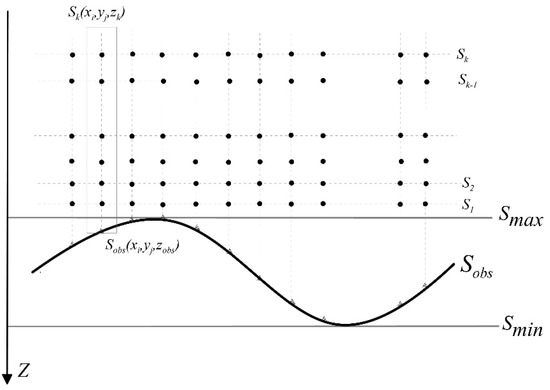
Figure 1.
is the observed surface, is the observed value at the location . is the surface through the highest height of and is the surface through the lowest height of . Thus, means the surface that, at the height of and is the value at the location of , where .
Thus, with the process of the Fourier transform and the upward continuation, we obtain , as stated in Equation (12), and then can be obtained as stated Equation (13):
In summary, the imaging process of the proposed improved DEXP method consists of three main steps, as described in this paper. Firstly, the elevation grid and G/M (gravity data or magnetism data) grid are read and defined. The first step involves using the hypothetical observed surface method to construct the 3D half-space field data. Next, the second step involves calculating the depth of extreme points using the adding constant method. Finally, the last step is the normalization process, as stated in Equation (8). Following these imaging steps, the imaging result can be analyzed to extract target characteristics, combine the other information (geophysics data, logging, metallogenic theory, geology evolution, and so on), and give the proper geological inference. Figure 2 illustrates the overall workflow of these steps.
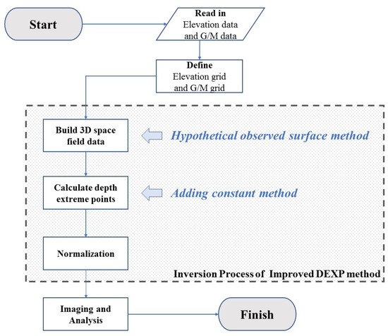
Figure 2.
Flowchart showing the improved DEXP method imaging process.
3. Application of Synthetic Data
To assess the performance of the proposed improved DEXP method, two types of synthetic models were selected: the single sphere and the combined spheres, as shown in Figure 3 and described in Table 1. In this section, we describe evaluations conducted to determine the possibility of mitigating the “zero area” effect using the synthetic models generated with flat terrain. Additionally, the synthetic data obtained with undulating terrain on the observed surface was used to test the validity of the improved DEXP method in the presence of topographic variations.
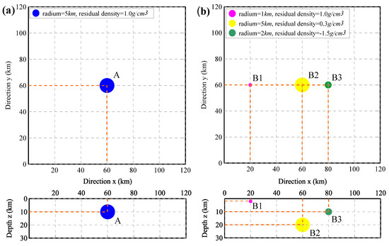
Figure 3.
The location and parameters of synthetic models. (a) The planar and sectional projection (y = 60 km) of the single-sphere model, Model A, the residual density is 1.0 g/cm3. (b) The planar and sectional projection (y = 60 km) of combined-sphere models, including Model B1, Model B2, and Model B3. The details of the parameters are listed in Table 1.

Table 1.
The parameters of the synthetic models.
3.1. Imaging Results for Flat Terrain
Figure 4a shows the Bouguer gravity anomaly data generated using the single model, Model A (shown in Figure 3a), for flat terrain. The cross-section is extracted using the model at y = 60 km. Figure 4b presents the imaging result of the DEXP method [9]. The extreme point at x = 60 km with a depth of 10 km coincides with the theoretical center of the sphere model. However, in Area I, delineated by the black line, significant “zero lines” are observed. These lines occur when the denominator in the DEXP method becomes zero. The presence of these “zero lines” is undesirable as they can be mistaken for additional extreme points, compromising the accuracy and reliability of the imaging result. In contrast, Figure 4c presents the imaging result obtained using the improved DEXP method proposed in this paper. The extreme point is located at x = 60 km with a depth of 10 km, coinciding with the theoretical center of the sphere model. The improved method ensures the reliability of inverted results. Furthermore, it is evident that the effect caused by the “zero line” can be suppressed, which will be beneficial in enhancing the quality of the imaging result.
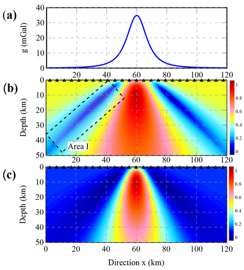
Figure 4.
The forward Bouguer gravity anomaly of Model A and imaging result of the main profile (y = 60 km) through Model A. (a) The forward Bouguer gravity anomaly observed for flat terrain. (b) The imaging result of the DEXP method. (c) The imaging result of the improved DEXP method.
Figure 5a shows the Bouguer gravity anomaly data generated using the combined model, consisting of Models B1, B2, and B3 (shown in Figure 3b), for flat terrain The cross-section is extracted through the models at y = 60 km. Figure 5b represents the imaging result obtained using the DEXP method, as shown in Area II. It is unfortunate that the center of Model B3 is not well recognized. This disturbance is caused by the empirically given threshold value, which is a constant value that cannot be adjusted automatically. Figure 5c presents the imaging result of the improved DEXP method proposed in this paper. This method, enhanced by the adding constant method, proves to be effective in obtaining reliable imaging results. Furthermore, the depth extreme points (x = 60 km, y = 60 km, depth = 10 km) accurately indicate the locations of the combined models.
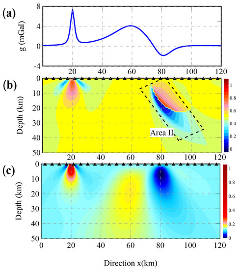
Figure 5.
The forward Bouguer gravity anomaly of Model B1, B2, and B3 and imaging results of the main profile (y = 60 km) through the combined model. (a) The forward Bouguer gravity anomaly observed for flat terrain. (b) The imaging result of the DEXP method. (c) The imaging result of the improved DEXP method.
3.2. Imaging Result for Undulating Terrain
Figure 6 depicts the imaging result obtained using the improved DEXP method with Model A. The extracted section is taken through the center of Model A at y = 60 km. To evaluate the validity and reliability of the improved DEXP method, a test was conducted using steep and undulating topography on the observed surface, ranging from 2 km to 10 km. The extreme points obtained from the method provide a satisfactory indication of the location of Model A, accurately capturing its features. Figure 7 presents a plot of the estimated depths from Figure 6 and calculates the error ratio. The statistical data demonstrate that the imaging results can achieve a highly reliable estimation of depth when the undulating terrain is below 5 km, which is five times the actual depth. However, as the topography becomes more pronounced, the accuracy diminishes. When the undulating terrain reaches 10 km, which is ten times the actual depth, the error ratio reaches 0.2.
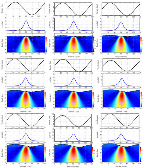
Figure 6.
Improved DEXP method imaging results of Model A for different undulating terrain (2–10 km).
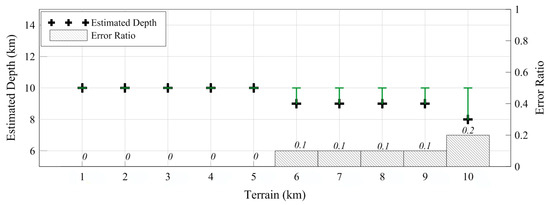
Figure 7.
The estimated depths shown in Figure 6 (the green symbol is the difference between the real depth and the estimated depth) and their calculated error ratio.
Figure 8 showcases the imaging results obtained using the improved DEXP method applied to the combined models, including Models B1, B2, and B3. The extracted section is taken through the centers at y = 60 km. The topography of the observed surface ranges from 1 km to 8 km. For Model B1, even as the degree of the terrain becomes stronger, the extreme points still possess the ability to identify the theoretical depth. The inverted horizontal location and depth are both in accordance with the theoretical parameters. When the observed surface is stronger than 6 km, the accuracy of the inversion decreases slightly, but the extreme points still provide a reliable indicator for the model. The method performs well in providing valuable imaging results for Model B2, which has the strongest anomaly. The recognition is obvious; however, the accuracy decreases as the undulating terrain becomes stronger, reaching 8 km on the observed surface. The signal becomes weaker, and there is some migration in the location of depth. In the case of Model B3, which has the medium–strong anomaly, the extreme point can still provide a referenceable location when the topography is below 2 km. However, the reliability of imaging results declines rapidly as the undulating terrain becomes stronger.
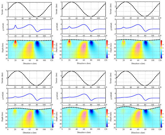
Figure 8.
The imaging result of the combined model with different step terrain (1–8 km).
4. Application on Real Gravity Data
The survey area for the potash salt deposit is situated on the eastern edge of the Sakhon Nakhon basin within the Korat Plateau in Laos. This region has garnered significant attention from explorers and researchers due to its abundant potash resources, as depicted in Figure 9. To validate the proposed method, we applied it to the residual gravity anomaly obtained from real ground relative-gravity survey data. The survey area covered approximately 291 km2 and was measured at a scale of 1:50,000. The grid distance between measurement points was set at 0.5 × 0.5 km, and the measurements were conducted using CG-5 gravitymeters (Scintrex Ltd., Concord, ON, Canada). To ensure accuracy, corrections were applied to the data, including tide correction, drift correction, latitude correction, height correction, mass correction, and terrain correction (the correction radium is 2 km). These corrections yielded the Bouguer gravity anomaly, with an accuracy of 0.042 × 10⁻⁵ m/s2. All the processes followed the technological standard outlined in “The Standard of 1: 50,000-scale Areal Gravity Prospecting, it is published by Ministry of Natural Resources of the People’s Republic of China”.
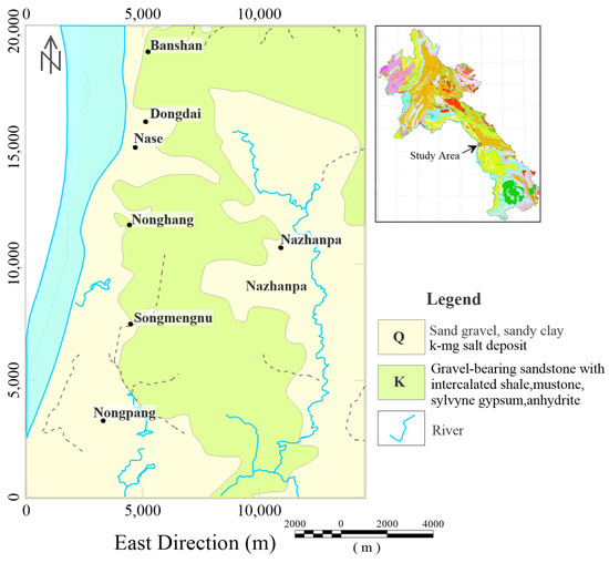
Figure 9.
The location and geological map of the study area (revised by Xiao, 2015 [39]).
To facilitate a more meaningful comparison, Profile I refers to a specific cross-sectional profile that was selected for analysis. The profile traversed Well Jx4 and Well Jx5, which are boreholes drilled in the survey area. By comparing the imaging results obtained from the improved DEXP method with the geological information derived from the borehole data, we aim to determine whether the imaging depth of the potash salt layer corresponds to the known geological layers.
Furthermore, we possess additional information regarding Well Jx4 and Well Jx5, both of which have been logged to identify potash layers. In Well Jx4, the rich potash layer is situated at a depth ranging from 132.5 m to 140 m. Following this, the potash salt layer extends from 140 m to 149 m. Consequently, the target rock exhibits a thickness of 16.5 m (132.5 m to 149 m). Well Jx5 features a rich potash salt layer ranging from 183 m to 187 m, succeeded by a potash salt layer spanning from 187 m to 254 m. Beyond that, there exists a layer consisting of potash salt and rock salt, extending from 254 m to 270 m. As a result, the target rock in Well Jx5 showcases significant thickness, amounting to 87 m (183 m to 270 m) (as illustrated in Figure 10). Within this survey area, the density of the potash salt deposit varies from 1.97 × 10³ kg/m3 to 1.99 × 10³ kg/m3, which is lower than the density of gypsum and rock salt, ranging from 2 × 10³ kg/m3 to 2.2 × 10³ kg/m3. The potash layer, exhibiting thickness ranging from a few meters to 80 m, is commonly found adjacent to the gypsum layer. Consequently, our objective is to analyze and interpret the low-density rock formations in order to accurately identify the potash layer.
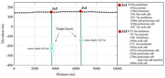
Figure 10.
The borehole data for Wells Jx4 and Jx5. With the analysis of known borehole data, the center depth of the Jx5 target layers is about 226.5 m, and the center depth of the Jx4 target layers is about 140.7 m.
The topography in the study area exhibits undulating characteristics, although it is not highly pronounced, with an elevation range of approximately 40 m (as depicted in Figure 11a). Figure 11b presents the residual gravity anomaly, which displays a high anomaly superimposed on the background of a relatively low anomaly. In the northern part of the study area, several higher-value anomalies are observed, forming localized traps amidst the overall high background anomaly. Furthermore, there exists a large-scale high-gravity anomaly between Songmengnu and Nongpang, which may be associated with the explosion of the old stratum. The gravity gradient zone predominantly follows a near NW trend, with the subsidiary trend in the NE and NNE direction. Near Nase and Nazhanpa, a linear structure is well developed with an NW trend, with subsidiary structures primarily developing in NE and trending NNE.
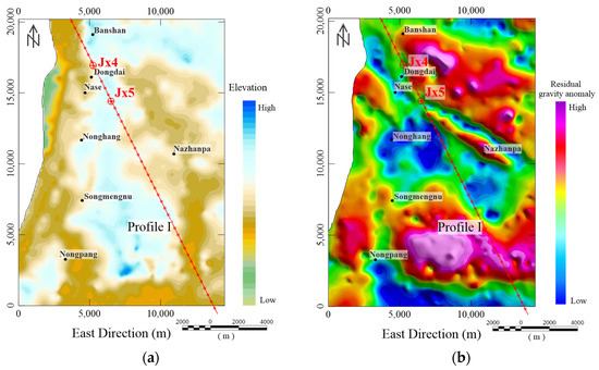
Figure 11.
(a) The elevation of the study area. (b) The residual gravity anomaly that was obtained. The study area is outlined with a white rectangle. Well Jx4 and Well Jx5 are known boreholes whose data are characterized by the potash salt deposit layers. To test the validity of the proposed method, Profile I (shown as the red line) is extracted and travels through Well Jx4 and Well Jx5, which is used for a comparison with the imaging result. The white rectangle is the range of gravity data.
The distribution of fault structure plays a significant role in the formation and occurrence of the potash salt deposit. Additionally, gravity prospecting offers distinct advantages in providing high-resolution information about the horizonal changes in the geological body. To detect the edge of the study area, we used the multidirectional standard difference method (CCMS method), which was proposed by Xu et al. [40]. This algorithm exhibits notable characteristics, including simplicity and stability, effective feature identification, accurate detection of the edges of geological bodies at various depths, robust preservation of edge shape, and low sensitivity to noise. The calculated result of the CCMS method is presented in Figure 12a, while the inferred fault structure is displayed in Figure 12b. It is evident that the tectonic structure is well-developed within the study area. The NW trending faults exert significant control near Wells Jx4 and Jx5, while sub-faults are observed in close proximity to Wells Jx4 and Jx5, with a near NE trending orientation. These fault structures play a crucial role in facilitating the formation and accumulation of potash salt.
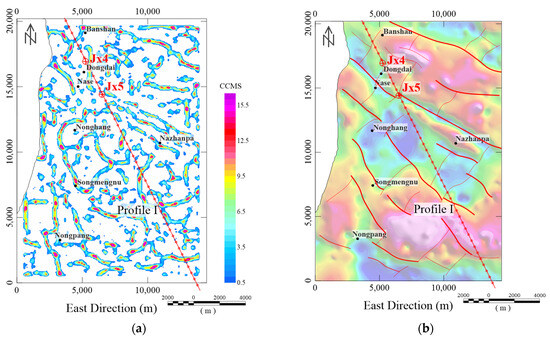
Figure 12.
(a) The inversion result of the CCMS method. (b) The distribution of the inferred fault (shown as red line) and the base map is the residual gravity (Figure 11b).
The imaging result of the improved DEXP method is shown in Figure 13. Figure 13b displays the combination of inferred faults and low-density rock, which is inverted using the improved DEXP method. It is evident that the location of low-density rock is significantly controlled by the faults, indicating the crucial role of fault structure functions in the sedimentary processes. Figure 13c illustrates the combination of the residual gravity anomaly, the lower value portion of the imaging result obtained using the improved DEXP method, and the inferred faults. The lower-value part of the imaging result represents relatively low-density rock. Furthermore, Figure 13d shows the extracted Profile I result from Figure 13c.
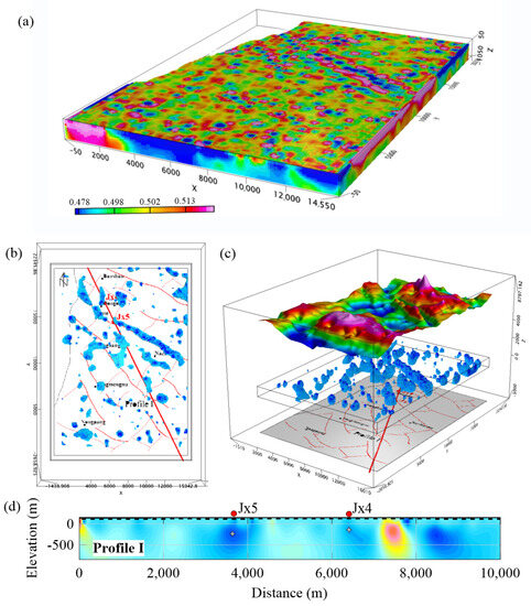
Figure 13.
The residual gravity anomaly, inferred faults, and imaging results obtained with the improved DEXP method. (a) The inversed result of the improved DEXP method. (b) The combination of the inferred faults and low-density rock. (c) The combination of residual gravity anomaly, and lower-value part of the imaging results obtained with the improved DEXP method and the inferred faults. (d) Extracted from the imaging result as Profile I, where the white cross points represent the low-extreme points. For Well Jx5, the depth of the low-extreme point is about 235.8 m; for Well Jx4, the depth of the low-extreme point is about 142.3 m.
In the Profile I result, it can be inferred that the depth of the low-extreme point in Well Jx5 is approximately 235.8 m (with an explored center depth of about 226.5 m). Similarly, the depth of the low-extreme point in Well Jx4 is estimated to be around 142.3 m (with an explored center depth of 140.7 m). By comparing these depths with the explored center depth, it is observed that the deviation in Well Jx4 is 0.7 m, resulting in an error ratio of 4.2% (error ratio = error/thickness). On the other hand, the deviation in Well Jx5 is 1.6 m, leading to an error ratio of 1.8%. Considering the objective of locating the potash salt layer, both the error and ratio fall within acceptable tolerances. Importantly, the inversed result of the improved DEXP method exhibits no significant disturbance, such as fake anomaly or “zero lines”. These advantages distinguish it from the pre-DEXP method. Additionally, no additional pre-SI value is required, highlighting its automatic calculation capability. These findings indicate that the imaging result obtained using the improved DEXP method is desirable and reliable. Furthermore, they suggest that this method can provide a valuable layer of information for interpretation.
5. Conclusions
We have proposed an improved DEXP method to address the problems associated with automatic calculation and undulating terrain. This method is based on a new definition that incorporates the adding constant method and hypothetical observed surface method. Using the tests conducted on the synthetic model, we demonstrated the flexibility and stability of this approach. Furthermore, we apply the improved DEXP method to real relative gravity data from potash salt deposits in the Sakhon Nakhon basin, Laos. The results of the application validate the effectiveness of this method in prospecting for potash salt deposits.
It is considered good practice to test the improved DEXP method on synthetic models. When the observed surface is flat, the inverted results of this improved DEXP method demonstrate satisfactory performance. The inverted locations and depths align well with the theoretical parameters, and importantly, the presence of disturbance from the “zero line” is effectively avoided, enhancing the reliability of the results. When the observed surface is undulating, the results obtained using a single model exhibit high flexibility, indicating the effectiveness and reliability of the improved DEXP method. In the case of combined models, the results still provide effective indicators, although the reliability varies depending on the intensity of different anomalies. It should be noted that as the undulation of the observed surface becomes more pronounced, the stability of the method decreases to some extent.
Next, it is important to highlight that the improved DEXP method was applied to real gravity data, and the results align well with the known borehole information, achieving an acceptable level of accuracy. This demonstrates the capability of the improved DEXP method to serve as a valuable tool for automated and reliable estimation of source depth and location. Additionally, by combining the edge detection method, we presented compelling evidence supporting the use of gravity data for effective potash deposit prospecting. This geophysical characterization based on gravity data further emphasizes the potential of gravity data as a valuable component in the prospecting process.
Clearly, the improved DEXP method demonstrates satisfactory validity and reliability for both synthetic data and real data. Notably, it eliminates the need for manual intervention in setting the SI or threshold value, ensuring stability in the imaging results by avoiding singularities or trapezoid lines. Moreover, it enables direct application to undulating terrain data, which enhances its practicality. However, it is worth mentioning that the accuracy of the method may be compromised when dealing with strongly undulating terrains. Despite this limitation, the proposed method remains significant and valuable for primary imaging of the target objects. It holds the potential to make a substantial contribution to the construction of detailed models for further geological research.
Author Contributions
Conceptualization, methodology, software, formal analysis, and writing: M.X.; gravity investigation: Y.W.; document editing: Y.Y. All authors have read and agreed to the published version of this manuscript.
Funding
This research was funded by the National Natural Science Foundation of China (grant numbers: 42104092), the Fundamental Research Funds Program of the Chinese Academy of Geological Sciences (grant numbers: JKYQN202351, JY202101), the China Geological Survey Project (grant numbers: GC20230111) and the China Scholarship Council (grant numbers: 202008575035).
Institutional Review Board Statement
Not applicable.
Informed Consent Statement
Not applicable.
Data Availability Statement
The data are not available.
Acknowledgments
This data-acquired work was carried out by Jilin University. Please allow us to show great appreciation to the editor and reviewer for their helpful comments and suggestions.
Conflicts of Interest
The authors declare no conflict of interest.
References
- Patella, D. Introduction to ground surface self-potential tomography. Geophys. Prospect. 1997, 45, 653–681. [Google Scholar] [CrossRef]
- Mauriello, P.; Patella, D. Gravity probability tomography: A new tool for buried mass distribution imaging. Geophys. Prospect. 2001, 49, 1–12. [Google Scholar] [CrossRef]
- Cui, X. Research on Probability Tomography of Geophysical Field. Master’s Thesis, Chinese University Geoscience, Beijing, China, 2009. [Google Scholar]
- Guo, L.H.; Meng, X.H.; Shi, L. 3-D correlation imaging for gravity and gravity gradiometry data. Chin. J. Geophys. 2009, 52, 1098–1106. [Google Scholar] [CrossRef]
- Guo, L.H.; Meng, X.H.; Shi, L. 3-D correlation imaging for magnetic anomaly ΔT data. Chin. J. Geophys. 2010, 53, 435–441. [Google Scholar]
- Meng, X.H.; Liu, G.F.; Chen, Z.X.; Guo, L.-H. 3-D gravity and magnetic inversion for physical properties based on residual anomaly correlation. Chin. J. Geophys. 2012, 55, 304–309. [Google Scholar] [CrossRef]
- Ma, G.Q.; Du, X.J.; Li, L.L. Improved Potential field Correlation Imaging method. Earth Sci. 2013, 38, 1121–1127. [Google Scholar]
- Zhdanov, M.S. Geophysical Inverse Theory and Regularization Problems; Elsevier Press: Amsterdam, The Netherlands, 2002. [Google Scholar]
- Fedi, M. DEXP: A fast method to determine the depth and the structural index of potential fields sources. Geophysics 2007, 72, I1–I11. [Google Scholar] [CrossRef]
- Zhao, G.X.; Wu, Y.T.; Sun, Y.; Zhang, B.B.; Zhou, X.; Wang, F.-J. Automatic DEXP method derived from Euler’s Homogeneity equation. Appl. Geophys. 2023, 1–8. [Google Scholar] [CrossRef]
- Florio, G.; Fedi, M.; Rapolla, A. Interpretation of regional aeromagnetic data by the scaling function method: The case of Southern Apennines Italy. Geophys. Prospect. 2009, 57, 479–489. [Google Scholar] [CrossRef]
- Moreau, F.; Gibert, D.; Holschneider, M.; Saracco, G. Wavelet analysis of potential fields. Inverse Probl. 1997, 13, 165–178. [Google Scholar] [CrossRef]
- Hornby, P.; Boschetti, F.; Horowitz, F.G. Analysis of potential field data in the wavelet domain. Geophys. J. Int. 1999, 137, 175–196. [Google Scholar] [CrossRef]
- Fedi, M.; Cella, F.; Quarta, T.; Villani, A. 2D Continuous Wavelet Transform of potential fields due to extended source distributions. Appl. Comput. Harmon. Anal. 2010, 283, 320–337. [Google Scholar] [CrossRef]
- Sailhac, P.; Gibert, D. Identification of sources of potential fields with the continuous wavelet transform: Two-dimensional wavelets and multipolar approximations. J. Geophys. Res. Solid Earth 2003, 108, 19455–19475. [Google Scholar] [CrossRef]
- Vallée, M.A.; Keating, P.; Smith, R.S.; St-Hilaire, C. Estimating depth and model type using the continuous wavelet transform of magnetic data. Geophysics 2004, 69, 191–199. [Google Scholar] [CrossRef]
- Antoine, J.P.; Murenzi, R.; Vandergheynst, P.; Ali, S.T. Two-Dimensional Wavelets and Their Relatives; Cambridge University Press: Cambridge, UK, 2004. [Google Scholar]
- Chen, Y.D. Inversion of gravity anomaly with continuous complex potential wavelet transform. Geophys. Geochem. Explor. 2003, 5, 354–361. [Google Scholar]
- Chen, Y.D. The identification of gravity anomaly with continuous complex potential wavelet transform. Geophys. Geochem. Explor. 2006, 2, 141–147. [Google Scholar]
- Fedi, M.; Pilkington, M. Understanding imaging methods for potential field data. Geophysics 2012, 77, G13–G24. [Google Scholar] [CrossRef]
- Abbas, M.A.; Fedi, M.; Florio, G. Improving the local wavenumber method by automatic DEXP transformation. J. Appl. Geophys. 2014, 111, 250–255. [Google Scholar] [CrossRef]
- Fedi, M.; Abbas, M.A. A fast interpretation of self-potential data using the depth from extreme points method. Geophysics 2013, 78, E107–E116. [Google Scholar] [CrossRef]
- Fedi, M.; Florio, G. Determination of the maximum-depth to potential field sources by a maximum structural index method. J. Appl. Geophys. 2013, 88, 154–160. [Google Scholar] [CrossRef]
- Cella, F.; Fedi, M.; Florio, G. Toward a full multiscale approach to interpret potential fields. Geophys. Prospect. 2009, 57, 543–557. [Google Scholar] [CrossRef]
- Abbas, M.A.; Fedi, M. Automatic DEXP imaging of potential fields independent of the structural index. Geophys. J. Int. 2014, 199, 1625–1632. [Google Scholar] [CrossRef]
- Henderson, R.G.; Cordell, L. Reduction of unevenly spaced potential field data to a horizontal plane by means of finite harmonic series. Geophysics 1971, 36, 856–866. [Google Scholar] [CrossRef]
- Naidu, P.S.; Mathew, M.P. Fast reduction of potential field measured over an uneven surface to a plane surface. IEEE Trans. Geosci. Remote Sens. 1994, 32, 508–512. [Google Scholar] [CrossRef][Green Version]
- Wang, Z.M.; Zhang, X.F. Theory of 3D potential field upward continuation observed with random undulated terrain. J. Jilin Univ. Earth Sci. Ed. 1980, 1, 94–98. [Google Scholar]
- Huang, Y.H. Boundary Element Method in Infinite Domain and Terrain Corrections in Gravity-Magnetic Interpretation. J. Fuzhou Univ. Nat. Sci. Ed. 1989, 17, 15–21. [Google Scholar]
- Kuang, Y.P.; Zhang, X.L. The boundary element method for three-dimensional magnetic field data conversion of curved-surface to horizontal-plane. Comput. Technol. Geophys. Geochem. 2008, 30, 216–220. [Google Scholar]
- Emilia, D.A. Equivalent source used as analytic base for processing total magnetic field. Geophysics 1973, 38, 339–348. [Google Scholar] [CrossRef]
- Battacharyya, B.K.; Chen, K.C. Reduction of magnetic gravity data on an arbitrary surface acquired in a region of high topographic relief. Geophysics 1977, 42, 1141–1430. [Google Scholar] [CrossRef]
- Ji, X.L.; Wang, W.Y. Experimental research using the frequency-domain dipole layer method for the processing and transformation of potential field on curved surface. Prog. Geophys. 2014, 9, 2669–2678. [Google Scholar]
- Cordell, L.; Grauch, V. Mapping basement magnetization zones from aeromagnetic data in San Juan bansin, New Mexico. In The Utility of Regional Gravity and Magnetic Anomaly Maps; Society of Exploration Geophysics: Houston, TX, USA, 1985; pp. 181–197. [Google Scholar]
- Guspi, F. Frequency-domain reduction of potential field measurements to a horizontal plane. Geoexploration 1987, 24, 87–98. [Google Scholar] [CrossRef]
- Liu, J.L.; Wang, W.Y. Reduction of potential field data to a horizontal plane by a successive approximation procedure. Chin. J. Geophys. 2007, 50, 1551–1557. [Google Scholar]
- Guan, Z.N.; Zhang, P.Q.; Yao, C.L. A new rapid surface to plane method of 3-D potential field data in large amount. Annu. J. Chin. Geophys. Soc. 1999, 1. [Google Scholar]
- Wang, Y.G.; Zhang, F.X.; Wang, Z.W. Taylor series iteration for downward continuation of potential fields. Oil Geophys. Prospect. 2011, 46, 657–662. [Google Scholar]
- Xiao, F. Study on gravity data processing method and apply it to sylvite mine exploration. Ph.D. Thesis, Jilin University, Changchun, China, 2005. [Google Scholar]
- Xu, M.L.; Yang, C.B.; Wu, Y.G.; Chen, J.-Y. Edge detection in the potential field using the correlation coefficients of multidirectional standard deviations. Appl. Geophys. 2015, 12, 23–34. [Google Scholar] [CrossRef]
Disclaimer/Publisher’s Note: The statements, opinions and data contained in all publications are solely those of the individual author(s) and contributor(s) and not of MDPI and/or the editor(s). MDPI and/or the editor(s) disclaim responsibility for any injury to people or property resulting from any ideas, methods, instructions or products referred to in the content. |
© 2023 by the authors. Licensee MDPI, Basel, Switzerland. This article is an open access article distributed under the terms and conditions of the Creative Commons Attribution (CC BY) license (https://creativecommons.org/licenses/by/4.0/).