Abstract
It is extremely important to gather the viscosity behavior of fluids accurately for industries and academia. There is no better method than viscosity measurement to detect changes in the specific characteristics of the materials. However, viscosity measurement is indeed a very sensitive process. In nature, fluids are involved in widely various containers, and they are affected by serious temperature deviations. It is a necessity for viscometers to have the capability to obtain accurate data from all types of containers of fluids even in serious temperature variations in order to understand the natural phenomena inside the fluids. Conventional viscometers mainly neglect the effect of sudden temperature deviations inside the fluids, or they need to use very expensive water bath systems that stabilize the temperature around the test fluids, which is not feasible at all. In this research, the effects of non-uniform temperature fields are analysed detailly to confirm that even in extremely limited amounts, serious viscosity and temperature deviations may occur. Experiments were performed in two parts. The first part was conducted using several thermocouples with different test fluids to find out the effects of thermal conduction and convection. For the second part, particle image velocimetry (PIV) was utilized to comprehend the flow movement within the test fluids. It was shown that even for small volumes and even in very controlled environments, an almost 35% viscosity measurement error (VME) occurs. Finally, as a solution to this problem, a new non-dimensional parameter called the Akpek number was proposed. The Akpek number enables the estimation of VMEs in any possible case. VME is a very crucial obstacle that has urgency to be illuminated by researchers and scientists to improve fluid characteristics. The main goal of this research is to illuminate the importance of this problem and offer a potential solution. The final results are supported by experimental data and numerical simulations using OpenFOAM.
1. Introduction
Viscosity is a critical parameter for defining fluid quality in various industrial, scientific, and engineering applications. The significance of viscosity lies in its direct correlation with a fluid’s performance, efficiency, and behavior within dynamic systems. High-quality fluids are characterized by consistent and predictable viscosities, as this property affects the overall fluid dynamics and heat transfer capabilities. For instance, in the field of lubricants and hydraulic fluids, appropriate viscosity ensures efficient energy transmission and reduces wear and tear on mechanical components [1]. Viscosity measurement is also used to detect contamination levels in lakes [2,3,4]. The viscosity level of a lake rises if the lake is contaminated. In chemical processes, the proper control of viscosity is vital for optimizing reaction rates and product yield [5]. Furthermore, in medical and pharmaceutical applications, the viscosity of fluids can impact drug delivery systems and patient safety [6]. In a similar manner, blood viscosity is utilized to comprehend cardiovascular diseases in medicine [7,8]. Therefore, understanding and defining fluid quality via viscosity assessment is imperative for ensuring optimal performance and reliability across diverse industrial sectors. There is no better method than viscosity measurement to detect changes in the specific characteristics of materials [9].
Viscosity measurement is a crucial aspect of fluid characterization, but it comes with its fair share of challenges. One of the primary difficulties lies in accurately measuring viscosity across a wide range of fluids, from low-viscosity liquids to highly viscous substances. Traditional methods like capillary viscometry and rotational viscometry may struggle to provide precise results for non-Newtonian fluids, which exhibit complex viscosity behaviors under different shear rates [10]. Moreover, the presence of suspended particles or bubbles in the fluid can further complicate viscosity measurements, leading to inaccurate readings [11]. In addition to these challenges, heat transfer effects can significantly impact viscosity measurements. Temperature changes can alter a fluid’s viscosity, and maintaining a consistent temperature throughout the measurement process is essential to ensure accurate results [12]. Non-isothermal conditions can induce temperature gradients within the fluid, leading to variations in viscosity readings. Researchers must carefully consider the impact of heat transfer on viscosity measurements and implement appropriate temperature control techniques to minimize potential errors. Addressing these difficulties and understanding the effects of heat transfer is crucial for obtaining reliable and meaningful viscosity data across various fluid systems.
In normal conditions, heating from the surrounding environment causes heat transfer [13,14,15]. The three fundamental modes of heat transfer are conduction, convection, and radiation [16]. In this research, heat transfer through radiation is not taken into account since its effect is negligible. The level of heat transfer is crucial to evaluate the accuracy of the viscosity measurement in almost all types of viscometers [17]. However, there are only a few studies available in the literature which focus on the viscosity measurement errors caused by the uneven temperature fields within the fluids [18,19,20,21]. This research includes a much expanded and deeper analysis of these previous studies.
In this research, the effects of non-uniform temperature fields are analysed detailly in order to confirm that even in limited amounts, serious viscosity and temperature deviations may exist. It is shown that even for small volumes and even in very controlled environments, an almost 35% viscosity measurement error occurs. The final results are supported by experimental data and numerical simulations using OpenFOAM [22]. Finally, as a solution to this problem, a new non-dimensional parameter for optimum heating speed called the Akpek number is proposed. The Akpek number enables the estimation of VMEs in any possible case, thus assisting researchers in calculating viscosities in any possible case.
2. Experimental Design
The experiments were performed in two parts in two different experimental beakers to prove that significant viscosity and temperature variations can occur even in very small volumes. The first part focused on understanding the effects of thermal conduction and convection by measuring the magnitude of the uneven temperature field within the test liquids using several thermocouples. The results were supported by several simulations. In the second part, Particle Image Velocimetry (PIV) was used to understand the flow motion within the test fluids. A much smaller sample cup was used to obtain better images. To achieve statistically accurate data, the experiments were carried out three times. Three different fluids with distinct viscosities were utilized throughout the experiments to evaluate the influence of temperature deviations on viscosity measurement.
The volume of the test cup used for thermal conduction and convection has a height of 20 cm and horizontal dimensions of 10.8 cm × 10.8 cm. Meanwhile, the volume of the test cup used for flow visualization is much smaller, with a height of 40 mm and horizontal dimensions of 64 mm × 24 mm. Figure 1 and Figure 2 show schematic diagrams of the experimental setups for thermal conduction and convection and for flow visualization, respectively.
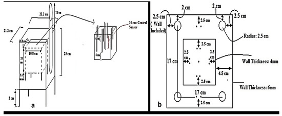
Figure 1.
Schematic illustration of experimental setup for thermal conduction and convection. (a) Front view. (b) Top view.
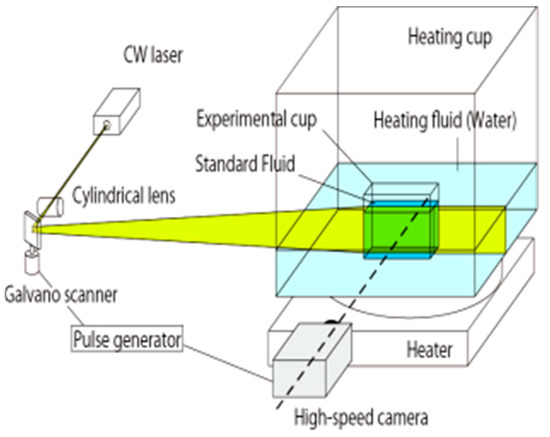
Figure 2.
Schematic illustration of experimental setup for flow visualization.
The heating cup has a volume of 11,236 cm3 for the thermal conduction and convection experiment and 3375 cm3 for the flow visualization experiment. The test fluids were introduced into the sample cups up to a height of 20 cm for the first experiment and up to 30 mm for the flow visualization experiment. In both experiments, the heights of the test fluids and the heating water were set to be equal to each other. The experiments were performed at room temperature.
2.1. Test Fluids
The test fluids used in the experiments are silicone oils purchased from Shinetsu Chemical Co. located in Yokohama, Japan. Their viscosity–temperature characteristics are presented in Figure 3. These fluids are denoted as Fluid A (KF-96-100 cSt), Fluid B (KF-96-1000 cSt), and Fluid C (KF-96H-10000 cSt), and have different kinematic viscosities of 100, 1000, and 10,000 mm²/s, respectively, at 25 °C. It is noteworthy that all three liquids have the same specific heat of 1.5 J/g·°C and a thermal conductivity of 0.16 W/m·°C despite their different viscosities.
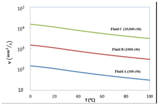
Figure 3.
Viscosity temperature graphic of Fluid A, B, and C.
2.2. Temperature Measurement in Thermal Conduction and Convection
As shown in Figure 4, a total of nine precise and calibrated thermocouples (accurate to ±0.02 °C) are strategically placed at various locations in the experimental beaker. The experimental cup is then placed in the center of a second cup, which serves as the heating cup. Water is used as the heating fluid, and six thermocouples are also placed in this heating beaker to ensure a uniform temperature of the heating fluid. To achieve controlled heating, the temperature of the heating fluid is gradually increased at a constant rate of 5 °C per minute, which is controlled by a 2500-watt resistor at the bottom and four 200-watt resistors (one at each corner) of the heating cup, as shown in Figure 4. It is expected that the use of five resistors can produce more homogeneous temperature fields, minimizing viscosity measurement errors. Throughout the experiments, the temperature values of all thermocouples are recorded simultaneously to analyze the temperature distribution in the fluid.
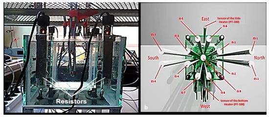
Figure 4.
(a) Experimental setup for analysis of thermal conduction and convection. (b) Schematic illustration of the experimental setup and placement of all sensors.
In this experimental setup, four thermocouples are located near the liquid surface at a depth of 5 cm, while another set of four thermocouples is located near the liquid bottom at a depth of 15 cm. In addition, a single thermocouple is placed in the center of the liquid at a depth of 10 cm. This detailed arrangement allows for a comprehensive analysis of the thermal fields within the sample cup. The thermocouple sensors within the sample cup are referred to as internal sensors (IS), while the sensors within the heating cup are referred to as external sensors (ES). In addition, the thermocouple in the center of the fluid is referred to as the central sensor. The sensors IS1, IS3, IS5 and IS7 are located near the surface, the sensors IS2, IS4, IS6 and IS8 are located near the bottom and the sensor IS9 is located in the center of the liquid.
2.3. Flow Visualization
To gain insight into the physical phenomena in the test cup, the velocity field is measured using Particle Image Velocimetry (PIV). The experimental setup for flow visualization is shown in Figure 5. To visualize the flow in the test fluid, a small amount of nylon tracer particles with a diameter of 20 μm and a specific gravity of 1.02 are introduced. Planar measurement of the velocity field is performed using a PIV system consisting of a CW Nd:YAG laser of 8 W power and a high-speed CMOS camera (1280 × 1024 pixels with 8-bit) operated by a pulse controller. The CMOS camera is positioned at a distance of 550 mm from the test cup. The frame rate of the camera is set to 130 frames per second with an exposure time of 7.6 ms. It is important to note that the camera lens has a focal length of 75 mm and an f-number of 2.8, while the thickness of the light sheet used for visualization is approximately 1 mm [23,24].
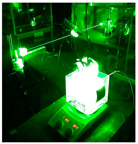
Figure 5.
Experimental setup for flow visualization.
To continuously monitor the temperature in the test cup, three thermocouples are strategically placed at different locations. The test cup is immersed in a heating cup during these temperature measurements. The thermocouples are specifically positioned along the longitudinal axis of the test cup, with one in the center and the other two near the wall. This arrangement allows comprehensive collection of temperature data from various points in the test fluid.
To ensure accuracy, these experiments are repeated three times, and the average values obtained from these repetitions are used to create a non-uniform temperature field for each liquid. The heating process is facilitated by a heating unit located under the heating water.
Throughout the experiments, the temperature readings of all three thermocouples are recorded simultaneously. The thermocouples are placed at a depth of 20 mm in the test fluid.
3. Mathematical Background
To understand the heat transfer phenomenon in the test cup, the Rayleigh number (Ra), the Grashof number (Gr) and the Prandtl number (Pr) are evaluated for the three fluids.
The Rayleigh number is defined by
the Grashof number is defined by
and the Prandtl number is defined as
where l is the characteristic length (distance of (IS1–IS9) in x coordinates), ΔT is the temperature difference between the surface and the center of the test fluid ((aritmetic average of IS1, IS3, IS5, IS7)–(IS9)), g is the gravitational acceleration, β is the volume expansion coefficient, ν is the kinematic viscosity and α is the thermal diffusivity. In addition, the Rayleigh number is simply the multiplication of the Grashof number and the Prandtl number (Ra = Gr × Pr).
For all fluids, the thermal diffusivity coefficient is 0.07 mm2/s, the expansion coefficient is 0.00095 (1/°C) and the gravitational acceleration is 9.8 m/s2. The kinetic viscosities at different temperatures are presented in Figure 3.
The heat distribution can be simulated in 3D using the heat equation [25]. For this purpose, a transient incompressible solver of the OpenFOAM platform is used, which implements the following temperature equation within the concept of thermal conduction:
In the given equation, T represents temperature, t represents time, and k represents the thermal diffusivity coefficient, which was set to 0.07 for the simulations. Figure 6 illustrates the computational geometry, where the four sides and the bottom part of the domain are defined as walls, while the top side is open to the atmosphere.
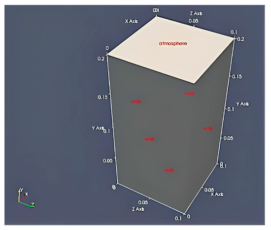
Figure 6.
Computational geometry of thermal conduction and convection experimental setup.
Figure 7 shows a carefully selected structured grid with 128,000 hexahedral cells generated using the blockMesh tool in OpenFOAM. This image shows the sensitivity analysis performed for the simulations and illustrates the influence and impact of the selected grid structure.
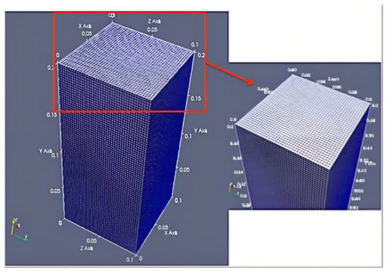
Figure 7.
A chosen structure grid.
Boundary conditions were carefully selected to be consistent with experimental settings. In particular, the temperature on the four sides and in the bottom part of the domain was gradually increased from 298 K to 363 K over a period of 10 min. In addition, the change in fluid viscosity was assumed to remain constant during the temperature increase due to the small magnitude of the change.
The calculations were performed on a PC equipped with an Intel Core i7 CPUX980 @ 3.33GHzX eight cores (each core with two threads) and 12 GB RAM. Each calculation required approximately 1.5 days to complete.
4. Results and Discussion
Figure 8 presents the change in Rayleigh, Grashof and Prandatl numbers through time.
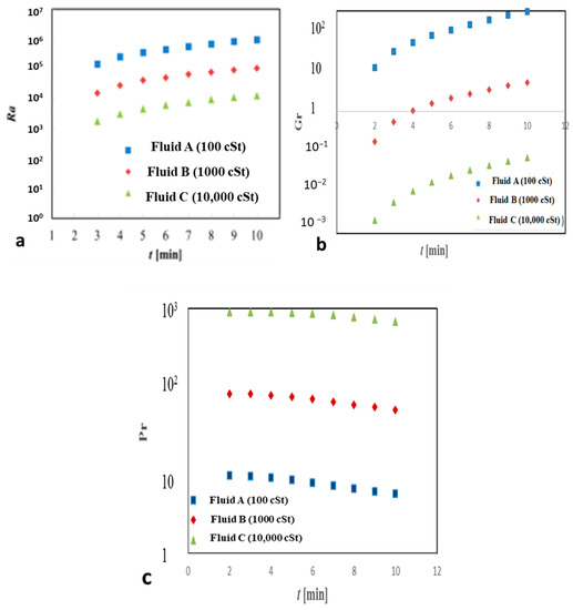
Figure 8.
Time variation in (a) Rayleigh number, (b) Grashof number, and (c) Prandtl number in measurements.
The temporal changes in the Rayleigh number for the test fluids show a rapid increase during the initial phase of heating, followed by saturation in the later phase. The Rayleigh number is a dimensionless parameter that is critical to the calculation of natural convection. The onset of convection occurs when the Rayleigh number reaches a critical value. Thus, it is an important indicator for determining whether natural convection is laminar or turbulent. It is simply the product of the Grashof number and the Prandtl number.
In this research, it should be noted that the Rayleigh number for test fluid A reaches approximately 106 in the later stages of heating, while it is about 105 for test fluid B, and about 104 for test fluid C.
The Grashof number is a parameter that helps us understand the turbulent regime within the fluid. A higher Grashof number indicates a turbulent boundary layer, while a lower Grashof number indicates a laminar boundary layer [26]. It is important to note that the Grashof number for liquid A exceeds 102 towards the end of the heating process. This means that after the eighth minute, thermal convection becomes more dominant than thermal conduction.
Furthermore, the Prandtl number is another significant parameter in our study. Smaller Prandtl numbers signify a greater effectiveness of thermal convection, while larger Prandtl numbers indicate a higher effectiveness of thermal conduction [27]. Our experimental findings demonstrate that as heating time increases, Prandtl numbers decrease, indicating that thermal convection becomes more dominant. Moreover, as the viscosity of the fluid decreases, the strength of thermal convection also increases.
Figure 9 confirms significant temperature variations between thermocouples in both the thermal conduction and convection experiments. These experimental results align with the mathematical outcomes based on Rayleigh, Prandtl and Grashof numbers. As the heating period increases, the temperature differences among the thermocouples of Fluid A become significantly smaller compared to Fluid B and Fluid C, indicating a decrease in the Prandtl number. With the Grashof number surpassing 102 for Fluid A, thermal convection becomes more dominant, resulting in smaller temperature fluctuations.
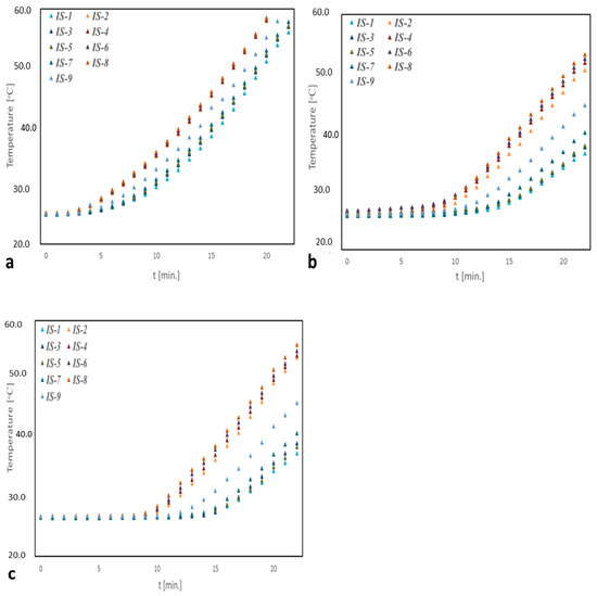
Figure 9.
Temperature assessment of (a) Fluid A (100 cSt); (b) Fluid B (1000 cSt); and (c) Fluid C (10,000 cSt).
Similarly, Fluid B and Fluid C exhibit smaller Rayleigh numbers, which are not significant enough to initiate turbulent flow within the fluids. As a result, laminar flow becomes dominant and causes larger temperature fluctuations between the thermocouples. On the other hand, the Rayleigh number of Fluid A is powerful enough to induce turbulent flow, leading to smaller temperature variations among the thermocouples. Meanwhile, the Rayleigh number of Fluid A is powerful enough to cause turbulent flow, representing smaller temperature variations between the thermocouples.
As a reminder, the measurement of temperature deviations is crucial for this research, as temperature deviations also mean deviations in viscosity.
Similar outcomes are presented from the flow visualization experiment. Figure 10 illustrates the temporal evolution of temperatures for the test fluids in the test cup, as well as the heating water, as recorded by the thermocouples. All temperatures gradually rise as time (t) progresses following the initiation of heating. Notably, the temperatures of the test fluid and the heating water are initially maintained at the same level during the onset of heating. While the relationship between temperature and time in the heating water remains unaffected by fluid viscosities, the temperatures (Tc and Tb) within the cup are influenced by the viscosity of the fluid. This effect becomes more pronounced for fluids with higher viscosities, leading to an increased temperature difference.
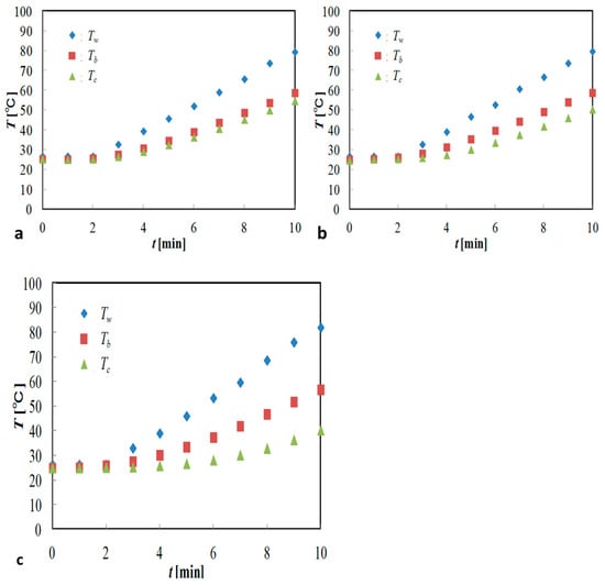
Figure 10.
Time variation in non-uniform temperature field in flow visualization test cup. (a) Fluid A (100 cSt); (b) Fluid B (1000 cSt); (c) Fluid C (10,000 cSt).
The heat transfer phenomenon for viscometers was also investigated through the numerical simulations using OpenFOAM. The simulations are shown in Figure 11 and Figure 12.
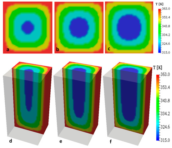
Figure 11.
Thermal conduction when t = 10 min in top view: (a) Fluid A (100 cSt), (b) Fluid B (1000 cSt), (c) Fluid C (10,000 cSt) and projectile view, (d) Fluid A (100 cSt), (e) Fluid B (1000 cSt), (f) Fluid C (10,000 cSt).
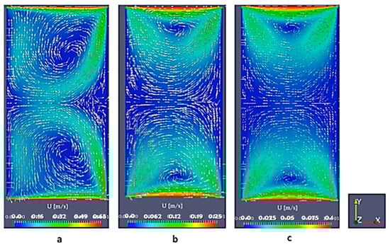
Figure 12.
Thermal convection when t = 10 min in (a) Fluid A (100 cSt), (b) Fluid B (1000 cSt), (c) Fluid C (10,000 cSt).
Figure 13 displays velocity field measurements within planar sections observed from the front and side of the test cup. These sections are taken through the center of Fluid A at the eight-minute mark, as captured during the current PIV experiment. The figure presents velocity vectors, magnitudes, and streamlines, providing insights into the flow dynamics within the test cup. Notably, the velocity magnitude (v) is depicted using color-coded bars. Importantly, it should be noted that the cell pattern exhibits asymmetry concerning the midplane. This asymmetry arises due to the considerable Rayleigh number of 6.6 × 10⁵, which induces flow instability [28].
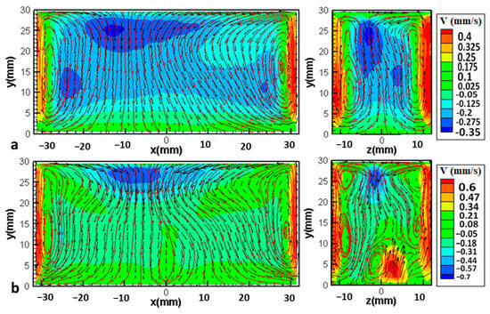
Figure 13.
Velocity field in test cup for Fluid A (100 cSt). (a) t = 4 min, (b) t = 8 min.
Figure 14 and Figure 15 show the velocity fields in the test cup for Fluids B and C, respectively, 8 min after the initiation of the heating. These results indicate that the magnitude of the thermal convection decreases as the viscosity of the fluid increases, corresponding to a decrease in the Rayleigh and Grashof numbers and an increase in the Prandtl number. Therefore, the influence of thermal convection becomes weaker for the highly viscous fluids and thermal conduction becomes the main method for the heat transfer. This result agrees well with the experimental observation of the temperature variations in the test cup and the estimates of the Rayleigh, Grashof and Prandtl numbers in Figure 6.
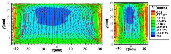
Figure 14.
Velocity field in test cup for Fluid B (1000 cSt) (t = 8 min).
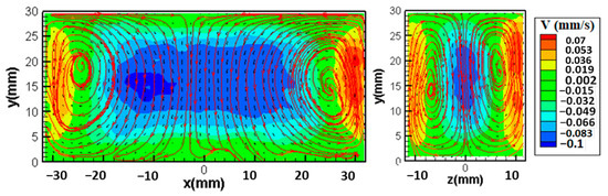
Figure 15.
Velocity field in test cup for Fluid C (10,000 cSt) (t = 8 min).
As a final discussion, VME graphic that is presented in Figure 16 explains a lot about the serious problems in viscosity measurement during heat transfer.
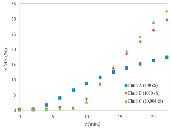
Figure 16.
Viscosity measurement error (VME).
VME is calculated by [29]
where is kinetic viscosity ( at T °C and −25 °C < T < −250 °C.
where and imply the viscosity of Fluid A, B or C at the points where IS8 (at the bottom) and IS1 (at the surface) measure the temperature (T) at selected times.
Owing to pronounced thermal convection, low-viscosity fluids offer a more thermally uniform environment, leading to reduced VMEs. Nevertheless, even within these favorable circumstances, there is still a 15% occurrence of VMEs. In the case of highly viscous fluids, the outcomes related to VMEs are notably more severe. As the duration of heating extends, the incidence of VMEs escalates, reaching levels as high as 30%, ultimately invalidating all viscosity measurements.
5. The Proposal of a Non-Dimensional Parameter Called the Akpek Number as a Possible Solution for VME
In the previous parts, the non-uniform temperature distribution problem was discussed. It is understood that this problem in viscometers is naturally caused by the thermal conduction and thermal convection.
In both industry and academia, capillary viscometers are widely used to obtain standard viscosity values. These values are universally accepted as highly accurate due to the absence of non-uniform temperature distribution issues in capillary viscometers. The temperature measurement error in these instruments is typically within the range of ±0.02 °C, ensuring precise viscosity measurements.
However, it is essential to note that capillary viscometers can only provide single-point viscosity measurements. To acquire data equivalent to continuous viscosity measurements, it often takes several days, requires a significant amount of labor force, and can be expensive.
Despite the precision of capillary viscometers, the limitation in achieving continuous viscosity data has led to the exploration of alternative methods that strike a balance between accuracy and efficiency. Researchers and industries are continually working to develop innovative techniques that can provide more frequent and cost-effective viscosity measurements without compromising accuracy.
In this section, a novel non-dimensional parameter is introduced to address the issue of non-uniform temperature distribution during fluid heating and its impact on viscosity measurements. The proposed concept suggests that there exists an optimal heating speed for a fluid, considering factors such as applied heat flux, viscosity change rate, fluid volume, and thermal diffusivity. By using this new concept, it becomes possible to eliminate the problem of non-uniform temperature distribution in viscometers. Consequently, any type of viscometer can provide viscosity measurements that are as accurate as those obtained with a capillary viscometer.
To calculate the acceptable heating speed that can eliminate the non-uniform temperature distribution problem, certain parameters need to be considered. These parameters include:
In Equation (7), x is location, t is time, Ti is initial temperature, Tf is final temperature, L is the length between the center and the edge of the fluid, α is the thermal diffusivity, is the viscosity change in temperature and is the change in the temperature of edge of the fluid in time.
By non-dimensionalizing these parameters, we can create a standardized equation that removes the dependence on specific units and scales. This will enable us to solve similar heating speed problems in a more general and applicable way.
In Equation (8), non-dimensional temperature parameter indicates the rate between (T and Tf) and the maximum temperature difference that is (Ti − Tf). Based on this, parameter Ɵ∗ should remain in the interval of 0 < < 1.
When x is non-dimensionalized,
Therefore, when t is non dimensionalized,
In Equation (10), is called the Fourier number.
When viscosity change in temperature () is non-dimensionalized,
In Figure 17, the centerline temperature of an infinite cylinder is plotted as a function of time. It can be observed that as the Fourier number increases, the temperature homogeneity also increases. In fluid mechanics, the Fourier number is a dimensionless parameter used to characterize heat conduction. Conceptually, the Fourier number represents the ratio of the conduction rate to the storage rate of heat and is derived from the non-dimensionalization of the heat conduction equation, as shown in Equation (12).
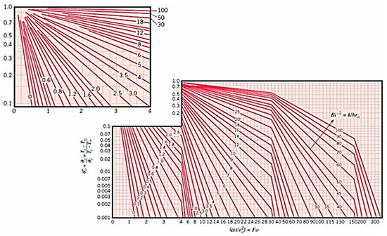
Figure 17.
Heisler chart and centerline temperature as a function of time [30].
The Fourier number plays a crucial role in understanding the heat transfer behavior in various systems. As it increases, it indicates that heat conduction becomes more dominant compared to heat storage effects, leading to a faster and more uniform temperature distribution within the system. This information is valuable for analyzing and solving heat conduction problems in different engineering and scientific applications.
The Fourier number includes the following parameters:
Fo = Fo (x, t, Ti, Tf, L, α).
Figure 18 and Figure 19 are presented as an example to the viscosity change in temperature () and the change in the temperature of the edge of the fluid in time ().
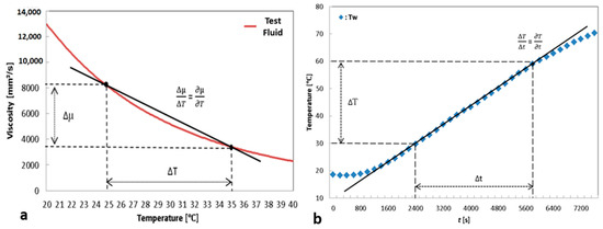
Figure 18.
(a) Viscosity change through temperature for a test fluid; (b) wall temperature change in time of a test fluid in low heating speed (0.5 °C/min). Black line emphasizes the difference among selected points.
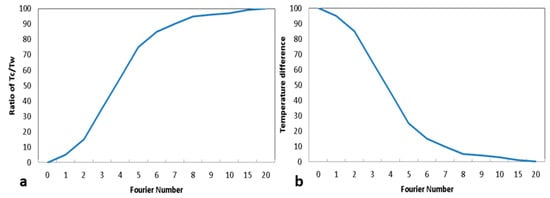
Figure 19.
(a) Ratio of Tc/Tw in percentage as the Fourier number increases. (b) Temperature difference as the Fourier number increases.
Based on the Heisler chart in Figure 17, temperature homogeneity (Ɵ∗) can be evaluated regarding to the change in the Fourier number.
As an example, let us say we have a ratio of center temperature (Tc) to wall temperature (Tw) in percentage as the Fourier number increases as in Figure 19a. In this figure, an inverse Biot number is accepted as zero.
This means we should have a temperature difference (1 − ) as in Figure 19b.
The viscosity change in temperature () and the wall temperature change in time () is directly proportional to the temperature difference. Therefore, viscosity change in temperature () and the wall temperature change in time () can only have a multiplication or a division effect in Figure 19b. After these parameters are added, the new graph appears as in Figure 20.
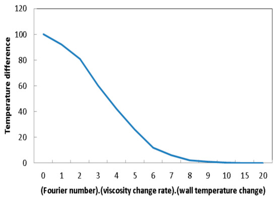
Figure 20.
Temperature difference and its relationship with Fourier number, viscosity change rate in temperature (), and the wall temperature change () in time.
To achieve a minimum error in temperature measurement, the Fourier number is assumed to be 1. Under this condition, the optimum settling time that results in the lowest temperature measurement error is determined.
By setting the Fourier number to 1, the study aims to determine the most suitable settling time that results in highly accurate temperature measurements. This finding is of great importance for improving the precision of viscosity measurements and contributes to the advancement of experimental methods in heat transfer analysis. Establishing an optimal settling time is a critical step in minimizing potential errors in temperature-dependent viscosity measurements, thereby improving the overall reliability and applicability of such analyses in various research and industrial contexts.
As a result, a new non-dimensional parameter known as the Akpek number emerges from the multiplication of the change in the viscosity by temperature (), the temporal variation in the edge temperature of the fluid (), and the time parameter derived from the Fourier Number.
For the special case where the Biot number is zero and the Fourier number is one, Figure 21 shows the relationship between the Akpek number and the viscosity measurement error, which is directly linear with the temperature difference. This graph is based on the data of the Heisler diagram.
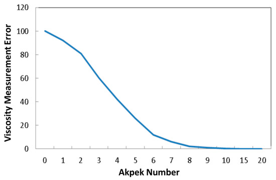
Figure 21.
Viscosity measurement error and the relationship with Akpek number.
This research result provides valuable insight into the influence of various parameters on viscosity measurement accuracy, especially in scenarios where temperature variation is significant. The Akpek number provides a comprehensive approach to quantifying the acceptable rate of heating and enables the design of effective heating systems and vessels for different types of fluids. The relationship presented between the Akpek number and viscosity measurement error serves as a practical guide for optimizing viscosity measurements in various experimental setups and industrial processes.
From the obtained results, it can be deduced that an Akpek number of about 9.5 is required to achieve zero viscosity measurement error for the sample fluid. The Akpek number serves as a crucial parameter in designing vessels or determining the heating rate for any type of fluid, either independently or interdependently. If the specific properties of the sample vessel are known, the Akpek number can be used to determine an optimum heating rate.
Moreover, the versatility of the Akpek number formulation allows its adaptation to different scenarios in which the Biot number or the Fourier numbers differ from the aforementioned values. By changing the t∗ number accordingly, the Akpek number can be adapted to different conditions, ensuring accurate viscosity measurements for a wide range of applications. This approach holds significant potential for improving the precision of viscosity measurements and facilitates the development of efficient heating systems for various liquid media.
6. Conclusions
The focus of this study is to investigate the effects of heat differences on viscosity measurements by examining non-uniform temperature fields in various experimental setups. The main objective is to understand the effects of heat convection and heat conduction phenomena on viscosity measurement. A comprehensive methodology is employed that includes mathematical principles of heat transfer, simulations, experiments, and Particle Image Velocimetry (PIV) results.
Results indicate that inherent errors in viscosity measurement can occur even with modern viscometers when temperature deviations are present. These errors can significantly affect the quality and production processes of various types of fluids. To address this problem, a non-dimensional parameter is proposed in this study. By incorporating this parameter into viscometers, viscosity measurements can be calculated more accurately regardless of the type of vessel, temperature variations, or properties of the viscous fluid. The proposed approach is promising for improving the accuracy of viscosity measurements and provides valuable insight for industries working with different fluid systems.
Funding
This study was supported by Yıldız Technical University Scientific Research Projects with the project number TSA-2022-5317. In addition, Dr. Ali AKPEK would like to thank Dr. Onur KOÇAK from IBUTEM Co. for designing the experimental setup presented in Figure 4. Also, Dr. Ali AKPEK would like to thank Dr. Barış BİÇER for providing simulations with Open FOAM in Figure 6, Figure 7, Figure 11 and Figure 12.
Institutional Review Board Statement
Not applicable.
Informed Consent Statement
Not applicable.
Data Availability Statement
The data presented in this study are available within the article.
Conflicts of Interest
The author declares no conflict of interest.
References
- Pabsetti, P.; Murty, R.S.V.N.; Bhoje, J.; Mathew, S.; Harivenkatesh; Rahul, K.; Feroskhan, M. Performance of hydraulic oils and its additives in fluid power system: A review. IOP Conf. Ser. Earth Environ. Sci. 2023, 1161, 012009. [Google Scholar] [CrossRef]
- Van Mullekom, J.H.; Melnyk, M.C.; Daya, B.S. Continuous On-Board Diagnostic Lubricant Monitoring System and Method. U.S. Patent 6,644,095, 11 November 2003. [Google Scholar]
- Ash, D.C.; Joyce, M.J.; Barnes, C.; Booth, C.J.; Jefferies, A.C. Viscosity measurement of industrial oils using the droplet quartz crystal microbalance. Meas. Sci. Technol. 2003, 14, 1955–1962. [Google Scholar] [CrossRef]
- Jakoby, B.; Scherer, M.; Buskies, M.; Eisenschmid, H. An automotive engine oil viscosity sensor. IEEE Sens. J. 2003, 3, 562–568. [Google Scholar] [CrossRef]
- Felder, R.M.; Rousseau, R.W. Elementary Principles of Chemical Processes; John Wiley & Sons: Hoboken, NJ, USA, 2016. [Google Scholar]
- Bashir, R.; Maqbool, M.; Ara, I.; Zehravi, M. An In sight into Novel Drug Delivery System: In Situ Gels. CellMed 2021, 111, e6. [Google Scholar]
- Lowe, G.D.O.; Lee, A.J.; Rumley, A.; Price, J.F.; Fowkes, F.G.R. Blood viscosity and risk of cardiovascular events: The Edinburgh Artery Study. Br. J. Haematol. 1997, 96, 168–173. [Google Scholar] [CrossRef] [PubMed]
- Devereux, R.B.; Drayer, J.I.; Chien, S.; Pickering, T.G.; Letcher, R.L.; DeYoung, J.L.; Sealey, J.E.; Laragh, J.H. Whole blood viscosity as a determinant of cardiac hypertrophy in systemic hypertension. Am. J. Cardiol. 1984, 54, 592–595. [Google Scholar] [CrossRef] [PubMed]
- Viswanath, D.S.; Ghosh, T.K.; Prasad, D.H.; Dutt, N.V.; Rani, K.Y. Viscosity of Liquids, Theory, Estimation, Experiment and Data; Springer: Berlin/Heidelberg, Germany, 2007; pp. 1–5. [Google Scholar]
- Bird, R.R.; Armstrong, R.C.; Hassager, O. Fluid Mechanics. In Dynamics of Polymeric Liquids; John Wiley & Sons: Hoboken, NJ, USA, 1977; Volume 1. [Google Scholar]
- Bokman, G.T.; Supponen, O.; Mäkiharju, S.A. Cavitation bubble dynamics in a shear-thickening fluid. Phys. Rev. Fluids 2022, 7, 023302. [Google Scholar] [CrossRef]
- ASTM D341-20e1; Standard Practice for Viscosity–Temperature Equations and Charts for Liquid Petroleum or Hydrocarbon Products. ASTM: West Conshohocken, PA, USA, 2020.
- Fujisawa, N.; Adrian, R.J. Three-dimensional temperature measurement in turbulent thermal convection by extended range scanning liquid crystal thermometry. J. Vis. 1999, 1, 355–364. [Google Scholar] [CrossRef]
- Fujisawa, N.; Funatani, S.; Katoh, N. Scanning liquid-crystal thermometry and stereo velocimetry for simultaneous three-dimensional measurement of temperature and velocity field in a turbulent Rayleigh-Bérnard convection. Exp. Fluids 2005, 38, 291–303. [Google Scholar] [CrossRef]
- Corvaro, F.; Paroncini, M. An experimental study of natural convection in a differentially heated cavity through a 2D-PIV system. Int. J. Heat Mass Transf. 2009, 52, 355–365. [Google Scholar] [CrossRef]
- Incropera, F.P.; DeWitt, D.P.; Bergman, T.L.; Lavine, A.S. Fundamentals of Heat and Mass Transfer, 7th ed.; John Wiley & Sons: Hoboken, NJ, USA, 2011; pp. 1–12. [Google Scholar]
- Ishida, H.; Momose, K.; Kimoto, H. Unsteady and chaotic characteristics of natural convection field in vertical slots at large Prandtl number. Heat Mass Transf. 2006, 42, 645–651. [Google Scholar] [CrossRef]
- Akpek, A.; Youn, C.; Maeda, A.; Fujisawa, N.; Kagawa, T. Effect of Thermal Convection on Viscosity Measurement in Vibrational Viscometer. J. Flow Control Meas. Vis. 2014, 02, 12–17. [Google Scholar] [CrossRef]
- Akpek, A.; Youn, C.; Kagawa, T. A Study on Vibrational Viscometers Considering Temperature Distribution Effect. JFPS Int. J. Fluid Power Syst. 2013, 7, 1–8. [Google Scholar] [CrossRef][Green Version]
- Akpek, A. Effect of non-uniform temperature field in viscosity measurement. J. Vis. 2016, 19, 291–299. [Google Scholar] [CrossRef]
- Akpek, A.; Youn, C.; Kagawa, T. Temperature measurement control problem of vibrational viscometers considering heat generation and heat transfer effect of oscillators. In Proceedings of the 2013 9th Asian Control Conference (ASCC), Istanbul, Turkey, 23–26 June 2013; pp. 1–6. [Google Scholar]
- OpenCFD® Is a Registered Trade Mark. Available online: http://www.opencfd.co.uk/ (accessed on 8 August 2023).
- Kiuchi, M.; Fujisawa, N.; Tomimatsu, S. Performance of a PIV system for a combusting flow and its application to a spray combustor model. J. Vis. 2005, 8, 269–276. [Google Scholar] [CrossRef]
- Raffel, M.; Willert, C.; Kompenhans, J. Particle Image Velocimetry, Practical Guide; Springer: Berlin/Heidelberg, Germany, 1998; pp. 1–146. [Google Scholar] [CrossRef]
- Holman, J.P. Heat Transfer, 8th ed.; McGraw-Hill: New York, NY, USA, 2001; pp. 90–93. [Google Scholar]
- Fendell, F.E. Laminar natural convection about an isothermally heated sphere at small Grashof number. J. Fluid Mech. 1968, 34, 163–176. [Google Scholar] [CrossRef]
- Kraichnan, R.H. Turbulent Thermal Convection at Arbitrary Prandtl Number. Phys. Fluids 1962, 5, 1374. [Google Scholar] [CrossRef]
- Castaing, B.; Gunaratne, G.; Heslot, F.; Kadanoff, L.; Libchaber, A.; Thomae, S.; Wu, X.-Z.; Zaleski, S.; Zanetti, G. Scaling of hard thermal turbulence in Rayleigh-Bénard convection. J. Fluid Mech. 1989, 204, 1–30. [Google Scholar] [CrossRef]
- Shin-Etsu. Silicone Fluid Technical Data KF-96 Performance Test Results; p. 7. Available online: https://www.shinetsusilicone-global.com/catalog/pdf/kf96_e.pdf (accessed on 16 May 2023).
- Janna, W.S. Chapter 4—Unsteady state heat conduction. In Engineering Heat Transfer, 2nd ed.; CRC Press: Boca Raton, FL, USA, 1999; pp. 195–196. [Google Scholar]


Disclaimer/Publisher’s Note: The statements, opinions and data contained in all publications are solely those of the individual author(s) and contributor(s) and not of MDPI and/or the editor(s). MDPI and/or the editor(s) disclaim responsibility for any injury to people or property resulting from any ideas, methods, instructions or products referred to in the content. |
© 2023 by the author. Licensee MDPI, Basel, Switzerland. This article is an open access article distributed under the terms and conditions of the Creative Commons Attribution (CC BY) license (https://creativecommons.org/licenses/by/4.0/).