Key Influencing Factors Identification in Complex Systems Based on Heuristic Causal Inference

Abstract

In complex systems constrained by multiple factors, it is very important to identify the key influencing factors for mastering the evolution and development law of a system and for obtaining scientific decision-making suggestions or schemes. At present, the method based on experimental simulation is limited by the difficulty of system model construction; DEMATEL (Factual Decision Trial and Evaluation Laboratory) is inevitably influenced by subjective factors. In view of this, we propose a novel model based on heuristic causal inference. By combining the network analysis in complex network science, the model defines the global/local causal pathway and the causal pathway’s length in the causal network and takes the causal pathway contribution degree as an indicator to measure the approximate causal effects. The model includes steps such as causal network learning, causal pathway contribution degree calculation, and key influencing factor identification. The model uses the Fast Causal Inference (FCI) algorithm with prior knowledge to learn the global causal network of the complex system and uses the heuristic causal inference to calculate the causal pathway contribution degree. The heuristic method draws on the idea of complex network topology analysis and measures the influence degree between variables by the number and distance of causal pathways. The key influencing factors are finally identified according to the causal pathway contribution degree. Based on the SECOM dataset, we carried out simulation experiments and demonstrated the feasibility and effectiveness of the proposed method.

1. Introduction

There are various complex systems in the fields of natural science and social science, such as atmospheric systems, computer networks, and human societies [1,2,3,4]. In these complex systems, there are numerous system factors, which are interrelated and work together on the operating state or output result of the system. However, there is no doubt that among all these factors, there are often a few that play a dominant role, which we call the key influencing factors [5,6]. In complex systems constrained by multiple factors, it is very important to identify the key influencing factors for mastering the evolution and development law of the system and for obtaining scientific decision-making suggestions or schemes [7].

In fact, to identify the key influencing factors in a complex system, we need deep knowledge and understanding of the system itself. On one hand, it requires long-term observation of the system; on the other hand, it requires the use of advanced technologies and methods to conduct scientific analysis of the system. The existing relevant methods include factor analysis [8], principal component analysis (PCA) [9], regression analysis [10], and so on. Among them, factor analysis is a qualitative analysis method based on the knowledge and experience of the analyst. Compared with the quantitative analysis method based on data, this method is more subject to subjective factors. Principal component analysis (PCA) is designed to find new variables that are linear functions of those in the original dataset. Finding such new variables, the principal components (PCs), requires solving an eigenvalue/eigenvector problem, which is often not feasible when there are too many variables in the dataset. Regression analysis is used to establish a regression model, obtain the model parameters according to the measured dataset, and express the relationship between variables via a mathematical analytic formula. When there is a large number of variables to be studied, this analytical formula is difficult or even impossible to solve. Therefore, although the above methods are widely used in the identification of key influencing factors, they are all targeted at cases with fewer variables. For example, the literature [11,12,13] used PCA or regression analysis to identify key influencing factors in different scenarios, and the datasets used only contained 5, 10, and 15 variables, respectively. The experimental simulation method and DEMATEL method are considered the two main methods used to identify the key factors influencing complex systems [14,15,16], but each has its own shortcomings, which will be discussed in detail in Section 2.

Complex networks abstract things graphically, which can help us understand complex systems from the perspective of the topology of interacting networks [17]. Causal inference, as a science in which the main goal is to discover causal relationships behind variables/things, is essential for rigorous decision making in the study of complex systems [18,19,20,21]. The above two methods draw on the formal methods of graph theory by using nodes and edges to describe variables and the relationship between variables, respectively. The deep integration of these two theories and methods helps to carry out more scientific and in-depth research on complex systems and other problems. When modelling complex systems, we can combine the ideas and methods of complex networks and causal network construction to draw the “real” structure of the organization. In network analysis, quantitative indicators such as the degree, degree distribution, and agglomeration coefficient of complex networks can be used for heuristic calculation of causal effects. When studying the dynamic characteristics of the network, the topological structure and causal transfer structure of the network can be considered at the same time to provide a scientific basis for the decision making of complex systems.

In this paper, to identify the key influencing factors in complex systems, we propose a model based on heuristic causal inference, which consists of three modules: causal network learning, heuristic causal effect calculation, and key influencing factor identification. Causal network learning enables us to re-understand the concerned system from the perspective of causation; heuristic causal effect calculation enables us to analyse the interaction between system variables quantitatively; and key influencing factor identification enables us to grasp the core joints of the system accurately. Based on the observation dataset, we confirm the validity of the proposed method.

The novel contributions of our work are summarized as follows:

(1) We propose a complex system modelling and analysis method combining causal science and network science. This method can be used to identify the key influencing factors of complex systems. Compared with the traditional method based on experimental simulation, the proposed method does not need to establish a system simulation model, so it has better applicability. Compared with the DEMATEL method, the method proposed is based on scientific analysis of data, which avoids the problem that experts’ subjective and qualitative judgements are difficult to quantify and lack persuasion.

(2) We propose a causal network learning method that combines prior knowledge. Observation datasets of complex systems often belong to high-dimensional and heterogeneous datasets, and it is difficult for traditional methods to learn causal networks from these datasets directly. We propose adding the prior knowledge to the FCI algorithm, which includes the causal direction that can be inferred in time (the cause always occurs before the result) and the causal relationship between the variables that have been verified experimentally and so on. By merging prior knowledge, we can obtain causal networks underlying high-dimensional data at a lower cost.

(3) We propose a heuristic causal effect calculation method to identify the key influencing factors of complex systems. Inspired by the ideas of network science, we define the concepts of causal pathway length and causal pathway contribution degree and propose a heuristic causal effect calculation method. This method draws on the idea of complex network topology analysis and takes the contribution degree of selected characteristic variables to the target variables on the causal pathway as an index to measure the approximate causal effect between variables. Depending on the size of the causal effect, the key influencing factors of the complex system can be identified effectively.

The rest of this paper is organized as follows: In the second section, we briefly introduce the relevant work. In the third section, the overall structure of the proposed model and the detailed technical method are introduced; in the fourth section, we describe the process and results of the experiment. The fifth section contains the analyses of the experimental results, and in the sixth section, we summarize the content of the paper and look forward to the next steps.

2. Related Work

Researchers are always interested in exploring kinds of complex systems. As mentioned earlier, the experimental simulation method and DEMATEL method are considered as the two main methods used to identify the key factors influencing complex systems. Among them, the experimental simulation method is mainly used in natural science, which is based on positivism. DEMATEL is mainly used in social science. It uses the methods of investigation, qualitative analysis, and quantitative calculation to identify the key factors influencing systemic problems in social activities.

2.1. Experimental Simulation Method

In the field of natural science, the experimental simulation method is used to construct a system simulation model for the target problem and to statistically analyse the influence of multiple factors on the system using variable control. On this basis, the key influencing factors of the system can be identified. In 2021, Rong et al. [22] established a mathematical model for the key components of the cross-delivery system of a launch vehicle. On this basis, the system simulation model was constructed by using professional software tools, and the key factors influencing the cross-delivery system were identified via modelling and simulation. In 2020, Zhang et al. [23] studied the static characteristics of double-cable suspension bridges based on the finite element analysis model, determined the key design parameters by calculating the effects of various parameters on the mechanical performance of the bridge, and put forward some specific suggestions for the design of such bridges. In 2013, Chen et al. [24] analysed the influence of four factors in space electronic equipment on the spectrum distribution of sound signals via a single-factor experiment and identified the key influencing factors using the orthogonal test method, which provided guidance for further identification of excess residues in the system. In 2021, Sun et al. [25] established a relevant chemical potential gradient model for struvite (MAP) crystal growth, identified four key influencing factors, and quantitatively analysed their effects on the growth rate of MAP crystals, thus providing a basis and guidance for the scientific regulation of the MAP crystallization process in industrial practice.

2.2. Factual Decision Trial and Evaluation Laboratory Method (DEMATEL)

In the field of social science, in the 1970s, American scholars Fontela and Gabus created DEMATEL (Factual Decision Trial and Evaluation Laboratory Method), which is based on graph theory and matrix theory, and conducted a comprehensive analysis of the internal correlation between multiple factors influencing complex systems [26,27,28].

In fact, DEMATEL is just one of several multiple-criteria decision analysis (MCDA) methods. In 2022, Basilio, M.P. et al. [29] conducted a complete review study on MCDA by using bibliometric analysis. MCDA can balance the relationship between many conflicting factors and is suitable for solving decision problems with multifactor constraints. Among them, the Analytical Hierarchy Process (AHP)/Analytical Network Process (ANP), Interpretative Structural Model (ISM), Technique for Order Preference by Similarity to an Ideal Solution (TOPSIS) and DEMATEL, or a combination thereof, have been widely used in multifactor analysis. In comparison, DEMATEL is superior to other methods in analysing factor causality because it provides the overall level of influence of each factor, as well as the interactions between them, and this network relationship can also be visualized for easy understanding [26,27]. The above characteristics of DEMATEL have good inspiration for the cause-based research idea proposed in this paper, so we focus on the novel abilities of DEMATEL and its technological applications. In practical applications, the method is deeply integrated with other methods and has been continuously improved and expanded [30,31,32,33,34,35,36].

In 2021, aiming at the identification of key influencing factors affecting the user experience of mobile reading apps, Zhang et al. [30] established a fuzzy DEMATEL model by introducing triangular fuzzy numbers and by extending the single value of the comparison matrix to the fuzzy interval, and they provided a suitable judgement space for decision makers. It effectively solved the defects of the traditional DEMATEL method in which the subjective deviation of expert judgement is large, and it is difficult to be directly expressed by accurate numbers. In 2022, Li et al. [31] constructed an evaluation index system in view of the institutional obstacles faced by China’s integration innovation, used the AHP-DEMATEL method to conduct an empirical analysis of this problem, identified key institutional obstacles such as the confidentiality system and intellectual property system, and provided countermeasures and suggestions for decision makers to carry out reform and innovation. In 2022, aiming at the problem of risk identification and control in enterprise product development, Chui et al. [32] combined network analysis with DEMATEL, established the ANP-DEMATEL model, studied the causal relationship between various risk factors and their relative importance, and identified six key influencing factors in the process of product development. In view of the important theoretical significance and application value of the DEMATEL method in the study of complex systems, Sun et al. [26,28] conducted a comprehensive study on the DEMATEL method from multiple perspectives, such as basic theory, operation logic, and cross-integration with other methods, and systematically reviewed the research status and development trends of the method. Their study is a reference and guide for subsequent theoretical research and practical applications.

In general, the above two methods have their own characteristics but also have their own limitations and shortcomings. The method based on experimental simulation has the characteristics of positivism, but it needs an established system simulation model, which is often difficult to achieve for complex giant systems. The DEMATEL method is focused on the analysis of the correlation between various factors influencing complex systems and is used to find the operation law of the whole system. However, its evaluation scale and determination of the self-dependence relationship between factors are greatly affected by subjective factors. Moreover, this method generally requires extensive research, which takes a long time and is more difficult.

With the construction and improvement in the big data environment in all walks of life, the evolution law of various complex systems is expected to be revealed via data science. At the same time, in recent years, the relevant methods of causal science have aroused great interest from scholars. Combining causal methods with observational data to reveal the nature of things has become a hot topic at present. In view of this, a heuristic causal inference method was proposed to address the problem of difficult identification of key influencing factors in complex systems. Experiments on semiconductor manufacturing datasets were carried out to verify the effectiveness of the method. Compared with the experimental simulation and DEMATEL method, the method proposed in this paper is more adaptable and feasible with the support of the observation dataset.

3. Proposed Method

According to the basic assumption of the DEMATEL method, we suppose a system has $n$ influencing factors, denoted as $S=\left\{s_{{}_1},s_{{}_2},\cdots ,s_{{}_n}\right\}$; there is a mutual influence relationship between these factors, and this relationship can be expressed in the form of a matrix. The initial direct influence matrix is constructed as $G={\left[g_{ij}\right]}_{n\times n}$ where $g_{ij}(i,j=1,2,\cdots ,n)$ is the degree of direct influence of factor $s_i$ on $s_j$ and $g_{ii}=0$.

In practical studies, it is common to focus on how one factor in the system is affected by other factors. We call the size of this impact the influence degree. In fact, there are many ways to measure the influence degree. In this paper, we use the number of paths between variables and the distance between variables to measure the influence degree, the specific implementation of which is detailed in Section 3.3. Let $t$ be the target variable that the researcher is interested in; $X=\left\{x_{{}_1},x_{{}_2},\cdots ,x_{{}_m}\right\}(m<n)$ is other system factors related to the target variable; the influence degree of $X$ on the target variable is recorded as $D={\left(d_l\right)}_{1\times m}$; and $d_l(l=1,2,\cdots ,m)$ is the influence degree of the factor $x_l$ on the target.

In descending order according to the value of $d_l$, the higher the ranking is, the greater the influence of the corresponding system factors on the target variables. According to this idea, several key influencing factors of the complex system can be identified.

3.1. Technical Framework

The essence of identifying the key influencing factors is to clarify the complex and nonlinear relationship among the factors in the complex system. With the support of an observation dataset, we adopt the methods of causal discovery and heuristic causal inference to solve the above problem. The overall technical framework of the research is shown in Figure 1.

The framework includes three key parts: causal network learning, heuristic causal inference, and identification of key influencing factors, which are further divided into seven steps. The first step is to obtain the original data, which is the basis of our research. We require the original data to conform to the general characteristics of complex systems; that is, the dataset consists of enough interrelated and interacting variables, and one of them can be regarded as the target of the system. The second step is to obtain experimental data. We pre-process the original data based on specific research ideas, including missing value processing, outlier value processing, and sampling processing, to form usable experimental data. In this process, we can eliminate some variables that are clearly irrelevant to the research content by combining prior knowledge. Step 3 is partially directed causal network learning, which mainly uses the FCI algorithm [37,38] to generate the initial causal network and combines prior knowledge and causal orientation rules to synchronously complete step 4, that is, global causal network construction. The fifth step is the construction of the adjacent local causal network of the target. The so-called adjacent local causal network refers to the target variable as the centre. Within a given order, it searches the causal variables connected with it, and the causal network composed of them is the adjacent local causal network of the target variable. We set that the order of an adjacent local causal network with a maximum causal pathway distance of $k$ (k ≥ 1) between the cause variable and the target variable is k. By referring to the concepts of “path” and “distance” in complex networks, the direct cause, indirect cause, and causal pathway length are defined, and the adjacent local causal network of the target variable is obtained via graph search. Step 6 is the calculation of the causal pathway contribution degree. The causal pathway contribution degree reflects the potential impact of cause variables (direct causes/indirect causes) on the target variable from the perspective of causal network topology analysis. It is used to comprehensively consider the number of causal pathways pointing to the target variable using cause variables and the distance of causal pathways from cause variables to the target. For its formal definition, see Definition 7 in Section 3.3. Based on defining the global causal pathway, local causal pathway, and average causal pathway’s length, we establish a heuristic causal effect calculation model to achieve an approximate calculation of causal effects among variables in the system. Step 7 is based on the calculated causal pathway contribution degree; the key influencing factors of the target are finally identified.

In the above research, steps 1–4 correspond to the completion of causal network learning, and steps 5–7 correspond to the completion of heuristic causal inference and identification of key influencing factors.

3.2. Causal Network Learning

In data science, the evolution and development of a system can be revealed using data analysis. In this section, we take the observed data as input and use the FCI algorithm combined with prior knowledge to learn the global causal network behind the data. On this basis, a network search method is used to obtain the adjacent local causal network around the selected target variable. The aim is to provide a trusted network structure for heuristic causal inference in the next section.

3.2.1. Global Causal Network Learning

Let $V=\left\{t,x_1,x_2,\cdots ,x_m\right\}$ be an $m+1$ dimensional set of variables in a given system $S$ where $t$ is the selected target variable and $\left\{x_1,x_2,\cdots ,x_m\right\}$ are the cause variables associated with $t$. Let $Q=\left\{q_1,q_2,\cdots ,q_p\right\}$ be the $p$ group observation datasets of $V$, and now it is necessary to discover the causal relationship between variables in $\left\{t,x_1,x_2,\cdots ,x_m\right\}$ based on the observation datasets. We use the FCI algorithm to learn the initial causal network among variables, combined with prior knowledge to supplement the orientation. The FCI algorithm is a classical method in the field of causal network learning that is suitable for high-dimensional and sparse causal network learning [39]. Combined with prior knowledge, it can further improve the efficiency of causal network learning. Finally, we obtain the global causal network. The basic steps are as follows:

Step 1: Use Algorithm 4.1 in [40] to learn the causal skeleton [41] ($\mathcal{C}$) between variables of the researched system and obtain the separate set [41] ($\mathcal{S}$) and the unmasked triplet [41] ($\mathfrak{M}$).

Step 2: Use Algorithm 4.2 in [40] to determine the orientation of the V-structure [41] in $\mathcal{C}$ and update it.

Step 3: Use Algorithm 4.3 in [40] to obtain the final causal skeleton, update it, and update the separate set ($\mathcal{S}$).

Step 4: Use Algorithm 4.2 in [40] to determine the orientation of the V-structure in $\mathcal{C}$ and update it again.

Step 5: Apply rules (R1)~(R10) in [42] to determine the causal orientation of the skeleton ($\mathcal{C}$) as much as possible and then update it.

Step 6: Use prior knowledge to conduct supplementary orientation for $\mathcal{C}$ and obtain the global causal network $\mathcal{G}.$

In the above causal discovery process, the hypothesis to be satisfied includes the following:

Causal Sufficiency Hypothesis.

The variable set V is causally sufficient when the direct cause variables of any two variables of V are also included in V.

Causal Markov Hypothesis.

For a set of variables that satisfies the causal sufficiency hypothesis, the set of variables satisfies the causal Markov hypothesis if every variable is mutually independent of its non-descendant nodes in the condition when its causal parent nodes are given.

Causal Loyalty Hypothesis.

If variables $x_i$ and $x_j$ are independent or conditionally independent under the premise of a given variable set $V$, then in the causal network $\mathcal{C}$ composed of variables and their causal dependency relationships, all pathways between $x_i$ and $x_j$ are d-separated by the appropriate variable in $V$. Then, the joint distribution $P$ of all random variables in $V$ is said to be causal loyalty to the network $\mathcal{C}.$

3.2.2. Adjacent Local Causal Network Construction

To identify the factors that have a key impact on the target, it is natural to search the adjacent local causal network of the target. The Markov blanket [41,43] is the most typical. For the convenience of description, the following definition is given first:

Definition 1.

Causal Operation Criterion—For causal variables A and B, it is assumed that the experimenter can manipulate variable A by setting its value to $a_e$, denoted as $do(A=a_e)$. If the experimenter observes that $P\left(B|do\left(A=a_e\right)\right)\ne P\left(B|do\left(A=a_f\right)\right)$ for some $e$ and $f$ (within the time window)$dt$, it indicates that $A$ is the cause of $B$ (within)$dt$.

Definition 2.

Direct and Indirect Cause—If $A$ is the cause of $B$ according to Definition 1, then $A$ is an indirect cause of $B$ with respect to a set $C,$ if and only if some assignment of $A$ to $C-\{A,B\}$ (by operation) is not a cause of $B$. Otherwise, $A$ is a direct cause of $B$.

According to the above definitions, for the target variable $t$, some variables in the global causal network are its direct causes and others are its indirect causes. Combined with the Markov blanket, the adjacent local causal network of the target variable $t$ can be constructed as follows:

Step 1: Choose the target variable $t$ and obtain its Markov blanket $\mathcal{J}$.

Step 2: Determine the order $k(k\ge 2)$ of the adjacent local causal network.

Step 3: Starting from the target variable $t$, search its direct and indirect causes within $k$ steps. Among them, the causal pathway length between the target and its direct cause is defined as 1.

Step 4: Take the target variable $t$ and its direct and indirect causes found in Step 3 as nodes, along with the edges between them, to build the adjacent local causal network.

3.3. Heuristic Causal Inference

With the global and adjacent local causal networks obtained above, we design a heuristic causal inference method to quantitatively calculate the causal pathway contribution degree of cause variables to the target variable.

In general, once a global causal network among variables is learned, the causal effects between variables can be calculated by using various graph search algorithms combined with quantitative causal inference methods. However, the calculation process is often very complex and is not feasible for large, dense causal networks. In view of this, a heuristic strategy for approximate causal inference is proposed.

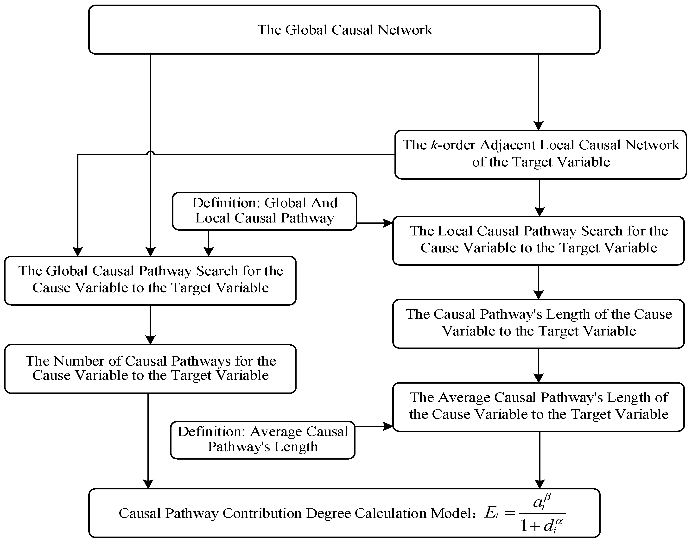
The basic idea of our method comes from a perceptual understanding of the physical structure of a causal network. In general, it can be inferred that the more causal pathways via a cause to the target, the greater the causal effect of the cause on the target. Under the same conditions, it can also be inferred that the shorter the causal pathway length of a cause variable from the target variable, the greater the causal effect of the cause on the target. Based on the basic understanding of the above two aspects, the framework of the heuristic causal inference model is shown in Figure 2.

For the convenience of expression, we provide the following definitions:

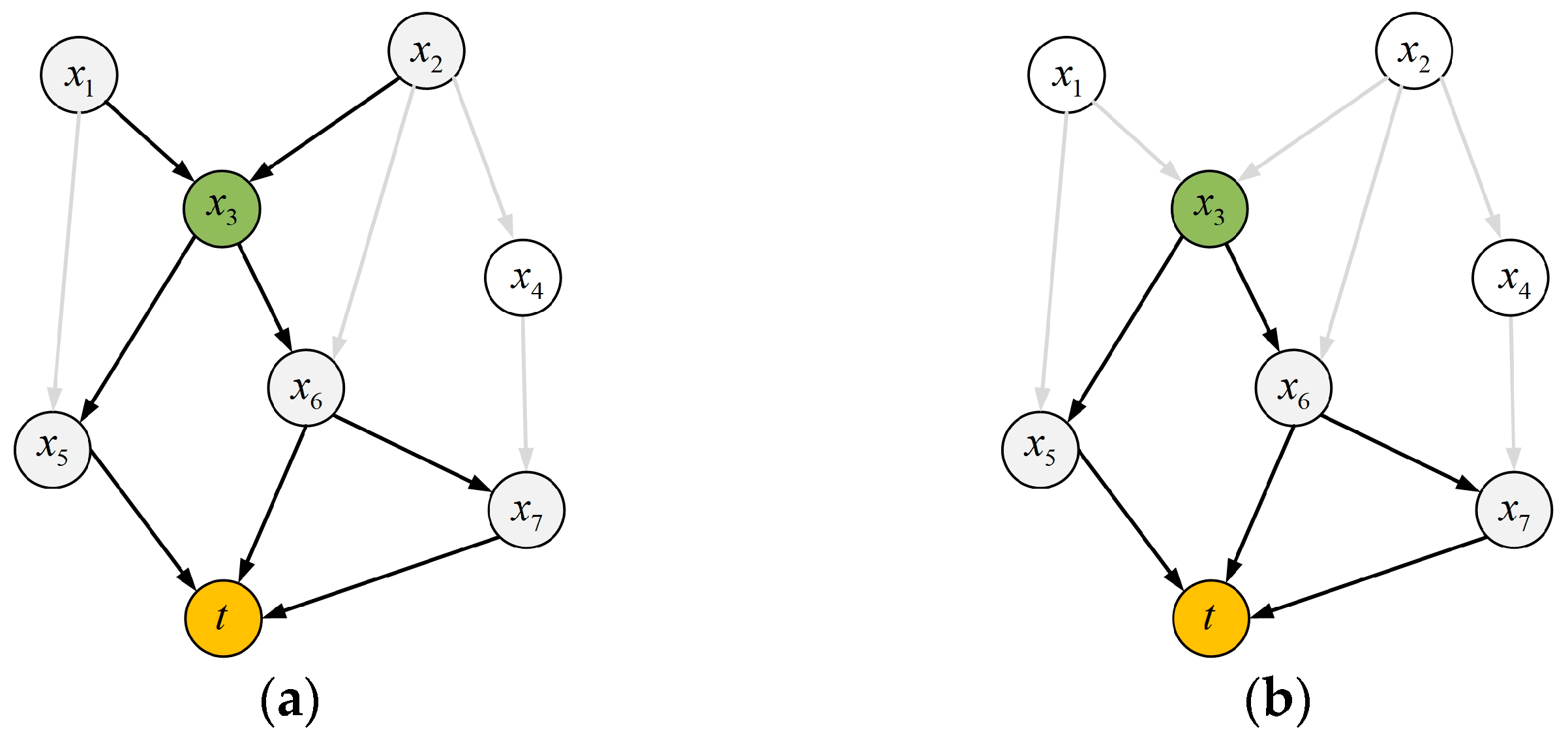
Definition 3.

Global Causal Pathway—In the global causal network, a variable $x_i\left(i=1,2,\cdots ,m\right)$ is the direct or indirect cause of the target variable $t$, and the causal pathway ($\cdots \to x_i\to \cdots \to t$) that points to the target variable $t$ through $x_i$ is defined as the global causal pathway from $x_i$ to $t$, as shown in Figure 3a.

Definition 4.

Local Causal Pathway—In the global causal network, a variable $x_i\left(i=\mathrm{1,2},\cdots ,m\right)$ is the direct or indirect cause of the target variable $t$, and the causal pathway ($x_i\to \cdots \to t$) that points to the target variable $t$ from $x_i$ is defined as the local causal pathway from $x_i$ to $t$, as shown in Figure 3b.

According to Definitions 3 and 4, if $x_i$ is an end node in a global causal network ($x_i$ has no parent), then the global causal pathway of $x_i$ is the same as its local causal pathway.

In Figure 3a, there are 9 global causal pathways from $x_3$ to $t$, including $x_1\to x_3\to x_5\to t$, $x_1\to x_3\to x_6\to t$, $x_1\to x_3\to x_6\to x_7\to t$, $x_2\to x_3\to x_5\to t$, $x_2\to x_3\to x_6\to t$, $x_2\to x_3\to x_6\to x_7\to t$, $x_3\to x_5\to t$, $x_3\to x_6\to t$ and $x_3\to x_6\to x_7\to t$. In Figure 3b, there are 3 local causal pathways from $x_3$ to $t$, including $x_3\to x_5\to t$, $x_3\to x_6\to t$ and $x_3\to x_6\to x_7\to t$. Thus, the global causal pathway of $x_3$ contains its local causal pathway.

Definition 5.

Local Causal Pathway’s Length—For a local causal pathway from $x_i$ to $t$, we define the total number of direct and indirect causes of $t$ on this pathway as the length of the local causal pathway.

In Figure 3b, the three local causal pathways from $x_3$ to $t$ have lengths of 2, 2, and 3, respectively.

Based on Definitions 4 and 5, the average causal path length can be defined as follows:

Definition 6.

Average Local Causal Pathway’s Length—We suppose there are $y$ local causal pathways from $x_i$ to $t$, and for the $w$th $\left(w=\mathrm{1,2},\cdots ,y\right)$ of them, its local causal pathway’s length is $d_{iw}$; and then, the average length of the local causal pathway from $x_i$ to $t$ is

$$d_i=\frac{\sum _{w=1}^y{d}_{iw}}{y}.$$

(1)

In Figure 3, the average local causal pathway length from $x_i$ to $t$ is (2 + 2 + 3)/3 = 7/3.

Based on Definitions 4 to 6, the causal pathway contribution degree of the cause variable to the target variable can be defined as follows:

Definition 7.

Causal Pathway Contribution Degree—In the global causal network, $\mathcal{G}$ , we assume that there are $a_i$ global causal pathways between the cause variable $x_i$ and the target variable $t$. Let the average local causal pathway’s length from $x_i$ to $t$ be $d_i$. Then, the causal pathway contribution degree of $x_i$ to $t$ is defined as

$$E_i=f\left(a_i,d_i\right).$$

(2)

where $f\left(·\right)$ is a monotonically increasing function of $a_i$ and a monotonically decreasing function of $d_i$, and $f\left(·\right)$ ≥ 0.

Without loss of generality, let

$$E_i=\frac{a_i^{\beta }}{1+d_i^{\alpha }}.$$

(3)

where α and β are adjustment factors greater than zero.

According to the above definitions, the causal effect of the cause variable $x_i$ on the target variable $t$ can be calculated approximately. The greater the value of $E_i$ is, the greater the causal effect of $x_i$ on $t$, and vice versa.

3.4. Key Influencing Factor Identification

If a certain target variable $t$ is selected in a complex system, there are several factors that have a large or small influence on it, and this influence can be measured using the causal effect value. Let the set of cause variables of the target variable $t$ be $X=\left\{x_1,x_2,\cdots ,x_m\right\}$, and these cause variables are the factors influencing $t$. In addition, let the causal effects of $x_i\left(i=\mathrm{1,2},\cdots ,m\right)$ on $t$ be $C_i\left(i=1,2,\cdots ,m\right)$; then, the greater the value of $C_i$ is, the greater the causal effect of $x_i$ on $t$. Usually, researchers pay more attention to the first several system factors that have a greater impact on the target variable. Here, these factors are defined as the key factors influencing the target variable $t$.

To identify the key factors influencing the target $t$, it is necessary to calculate the causal effect of the cause variable $x_i$ on $t$. According to the basic ideas in Section 3.3, the causal effect can be approximately replaced by the causal pathway contribution degree proposed:

$$C_i\approx E_i.$$

(4)

The longer the causal pathway is, the smaller the causal effect of the end cause variable on the target variable tends to be. Therefore, in the above calculation, the cause variable can be limited to the $\mathrm{k}$-order adjacent local causal network of the target variable $t$.

We sort the cause variables $x_i\left(i=\mathrm{1,2},\cdots ,q;q\le m\right)$ of $t$ in $t$’s k-order adjacent local causal network according to their causal effects on the target variable $t$. The rearranged sequence of cause variables is

$$\acute{x_1},\acute{x_2},\cdots ,\acute{x_q}.$$

Assuming that for a certain system only the first $r(r\le q)$ factors have a decisive influence on the target variable $t$, the key influencing factors identified based on the proposed method are as follows:

$$\acute{x_1},\acute{x_2},\cdots ,\acute{x_r}.$$

Among them, $\acute{x_1}$ has the greatest influence on the target variable $t$, $\acute{x_2}$ has the second greatest influence on the target variable $t$, and so on.

4. Experiments and Results

A semiconductor production system is taken as an example for the simulation experiment. In modern semiconductor production, quality control is often performed by monitoring signals collected from all kinds of sensors. In a specific monitoring environment, the monitoring signal reflects the operation of each node of the production line and determines the final product quality. If each type of signal is treated as a feature, there is a tight interrelationship between these features. By using the heuristic causal inference method proposed by our research, the causal relationship between characteristic variables is found; moreover, the key factors leading to the fluctuation of product output, chosen as the target variable and labelled as pass/fail, are finally identified.

The body of the method presented in this article is programmed in Python 3.10. Post analysis and network visualization were conducted mainly in Cytoscape 3.9.1.

4.1. Experimental Data Introduction and Processing

The experimental dataset SECOM [44] (Semiconductor Manufacturing) is derived from the UC Irvine machine learning repository. SECOM consists of production line monitoring data and semiconductor quality data, containing 1567 observations, each of which is a vector of 590 sensor measurements, plus a pass/fail label of the product.

Notably, there are some missing values in the dataset, and only 104 of the 1567 observations recorded that the product failed the quality test, while the vast majority of products passed the quality test with a ratio of approximately 1:14. To this end, the experimental data were pre-processed, and the main work included (1) establishing the index of the dataset; (2) deleting columns with more than 50% of their data missing; and (3) interpolating missing values in the dataset. In general, the missing values of each sample were imputed by using the mean value from n-neighbours found in the dataset. (4) We normalized the dataset by using the Max–Min normalization method. (5) We eliminated features that had a variation below a specified threshold, and (6) down-sampling technology was used for data balancing.

After processing, a new experimental dataset was formed, including 449 variables, and the sample size was 416 (the ratio of pass and fail was 3:1).

4.2. Global Causal Network Learning

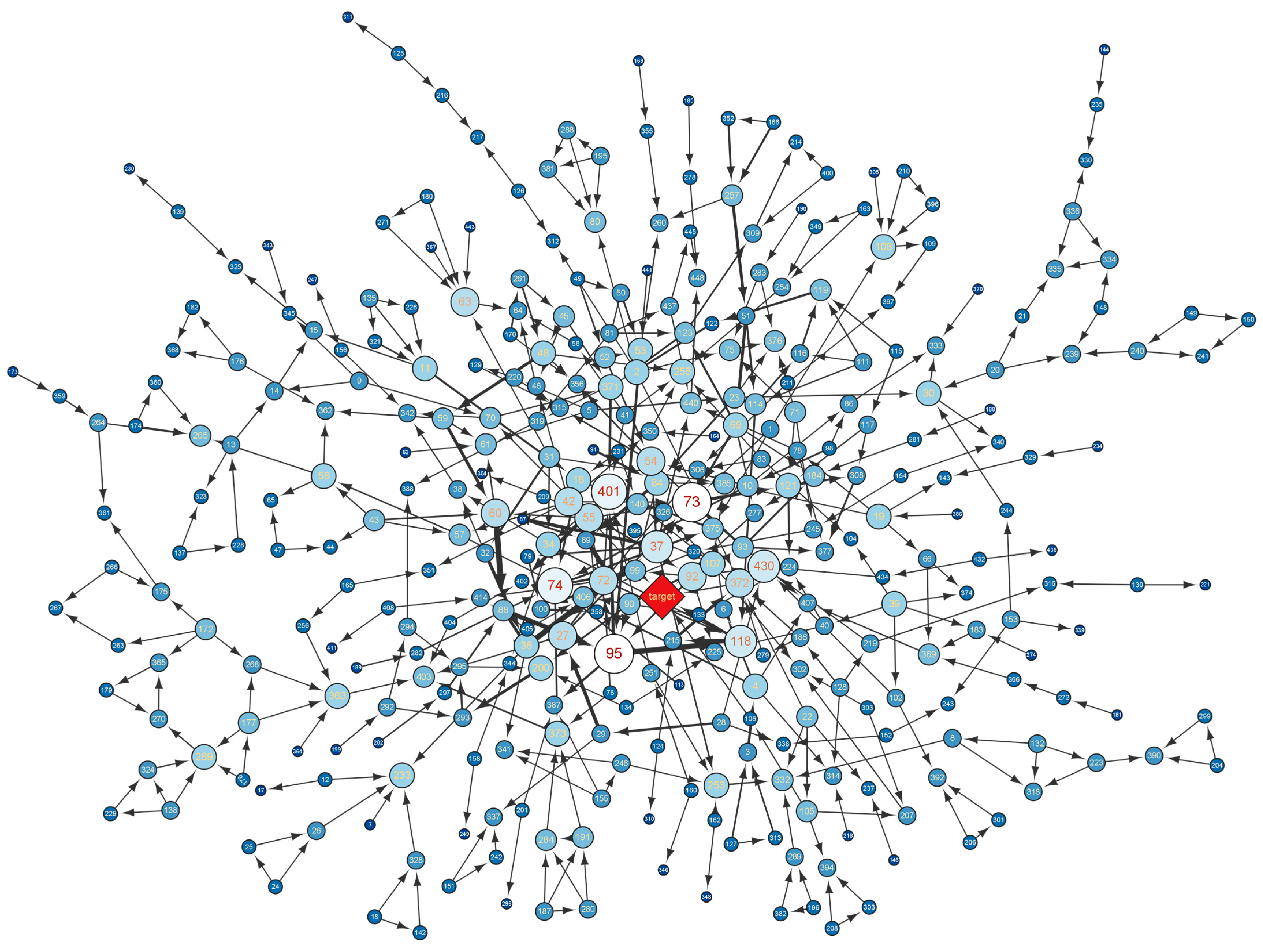
The experiment was carried out according to the steps described in Section 3.2.1. In the process, the significance level of FCI was set to 0.05, and other parameters were set to default. We obtained the global causal network around the target variable, as shown in Figure 4, including 347 nodes and 493 edges. where the central node “target” was the selected target variable, which refers to the product test results. The five surrounding nodes (55, 106, 118, 277, and 372) form the Markov boundary [42] of the target variable.

The global causal network was analysed in Cytoscape, and its network characteristics [45] are shown in

Table 1. Network characteristics of the global causal network.

Nodes	347
Edges	493
Average number of neighbourhood nodes	2.841
Network diameter	9
Characteristic path length	2.846
Network density	0.004

.

4.3. Local Causal Network Construction

According to the steps in Section 3.2.2, a third-order adjacent local causal network of the target variable was constructed, as shown in Figure 5.

In this third-order adjacent local causal network, there are 32 direct and indirect causal nodes of the target variable. There are five direct cause nodes whose shortest causal pathway length with the target variable is 1 (Markov boundary of the target variable). There are 13 indirect cause nodes whose shortest causal pathway length with the target variable is 2. There are 14 indirect cause nodes whose shortest causal pathway length with the target variable is 3.

4.4. Heuristic Causal Effect Calculation

According to the steps in Section 3.3, the number of causal pathways, average causal pathway length, and causal pathway contribution degree of each direct and indirect cause of the target variable in the adjacent local causal network were calculated, and the results are shown in

Table 2. Heuristic causal inference results in the adjacent local causal network (α, β = 1).

Node	Number of Local Causal Pathways	Number of Global Causal Pathways	Average Causal Pathway Length	Causal Pathway Contribution Degree
2	1	1	2	0.33
4	2	10	4	2
6	2	12	3	3
22	2	2	2.5	0.57
27	6	18	5.33	2.84
31	4	4	6.5	0.53
34	2	4	3	1
51	4	20	3.75	4.21
53	2	16	4	3.2
55	5	5	4.2	0.96
69	2	12	2.5	3.42
72	2	10	3	2.5
76	2	2	4	0.4
88	2	40	4	8
90	3	21	4	4.2
92	3	6	4	1.2
93	1	10	3	2.5
95	2	84	3	21
105	1	2	2	0.67
106	1	3	1	1.5
111	2	2	4	0.4
114	2	14	3	3.5
118	2	126	2	34
124	1	1	3	0.25
128	2	2	3.5	0.44
184	1	19	2	6.33
186	2	4	2.5	1.14
215	1	65	2	21.67
277	1	26	1	13
279	1	3	2	1
281	1	2	3	0.5
372	1	73	1	36.5

.

4.5. Final Results

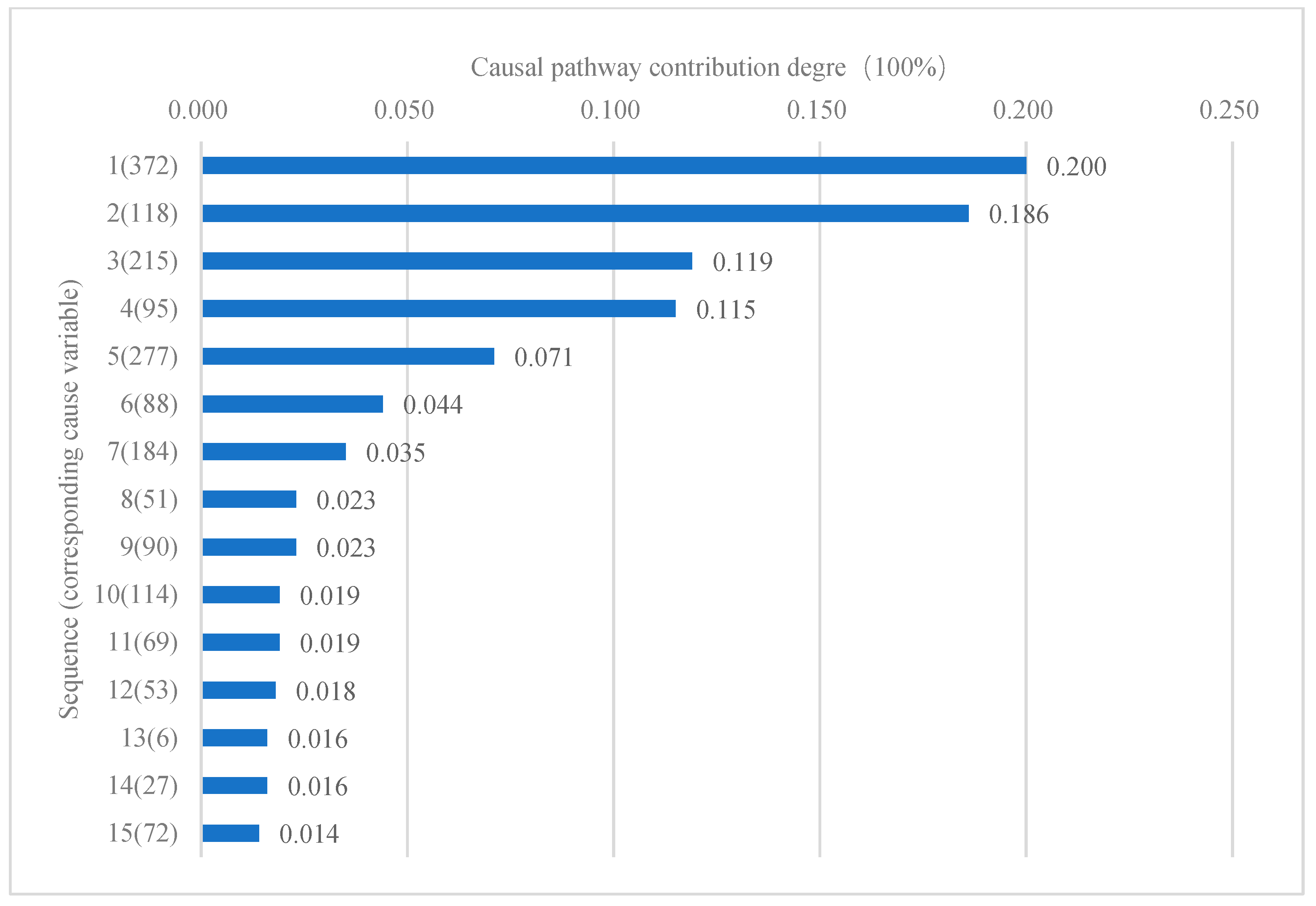
The causal path contribution degree in Table 2 is converted to percentages (the total impact of all nodes in Table 2 on the target node is 100%), and the top 15 influencing factors that have a greater impact on the target variable are screened out and sorted according to the ideas in Section 3.4. The results are shown in Figure 6. In the figure, node No. 372 is ranked first, and its causal pathway contribution degree is 19.97%. The second node is No. 118, whose causal pathway contribution degree is 18.60%. By analogy, the 15th ranked node is No. 72, whose causal pathway contribution degree is 1.37%.

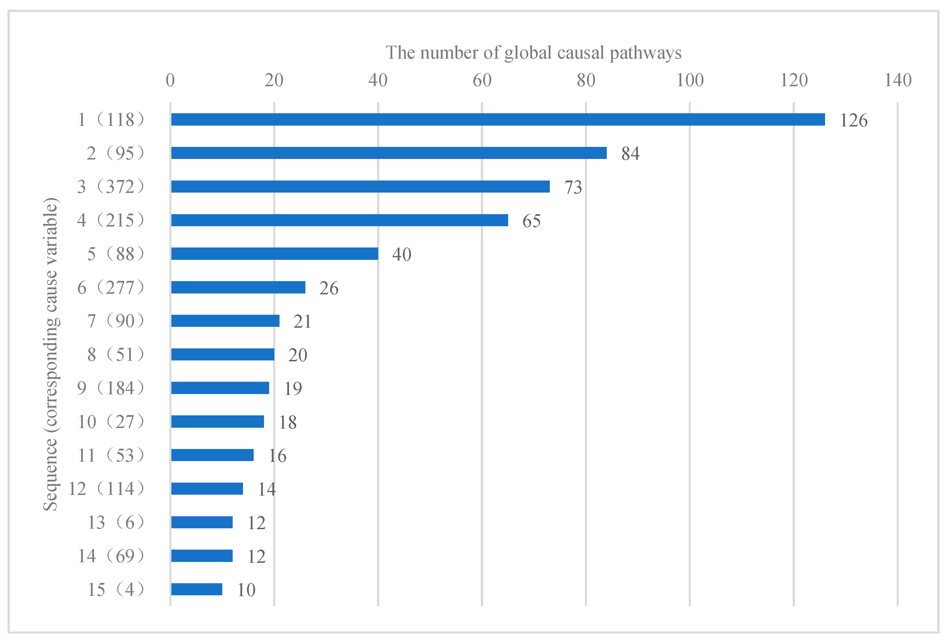
In addition, if only the number of causal pathways to the target variable is considered, the selected key influencing factors of the target variable are shown in Figure 7. At this time, the first node is No. 118, and there are 126 global causal pathways through this node to the target variable. The second node is No. 95, and there are 84 global causal pathways to target variables through this node. By analogy, the fifteenth is node 4, and there are 10 global causal pathways through this node to the target variable.

In order to verify the influence of the values of $\alpha$ and $\beta$ on the experimental results, we perform calculations when $\alpha =0$.5, $\beta$ = 1 and $\alpha =1$, $\beta =0.5$. It was found that under the different values of A and B, the identified key influencing factors basically did not change, but their order was slightly adjusted.

4.6. Further Validation

Thus far, we have screened out several key influencing factors. To verify the effectiveness of the proposed method, we refer to the evaluation metrics in feature selection and feature extraction [46,47] to evaluate the experimental results.

Since our dataset was highly imbalanced, we did not use accuracy as our evaluation metric. Instead, we used the F1 score and the Matthews correlation coefficient (MCC), which are both suitable measures of models tested with imbalanced datasets [48]. The F1 score is a comprehensive evaluation index that integrates two evaluation parameters, the accuracy rate and recall rate, to evaluate the overall performance of the classifier [49]. The MCC is essentially a correlation coefficient value between −1 and +1. A coefficient of +1 represents a perfect prediction, 0 is an average random prediction and −1 is an inverse prediction [50].

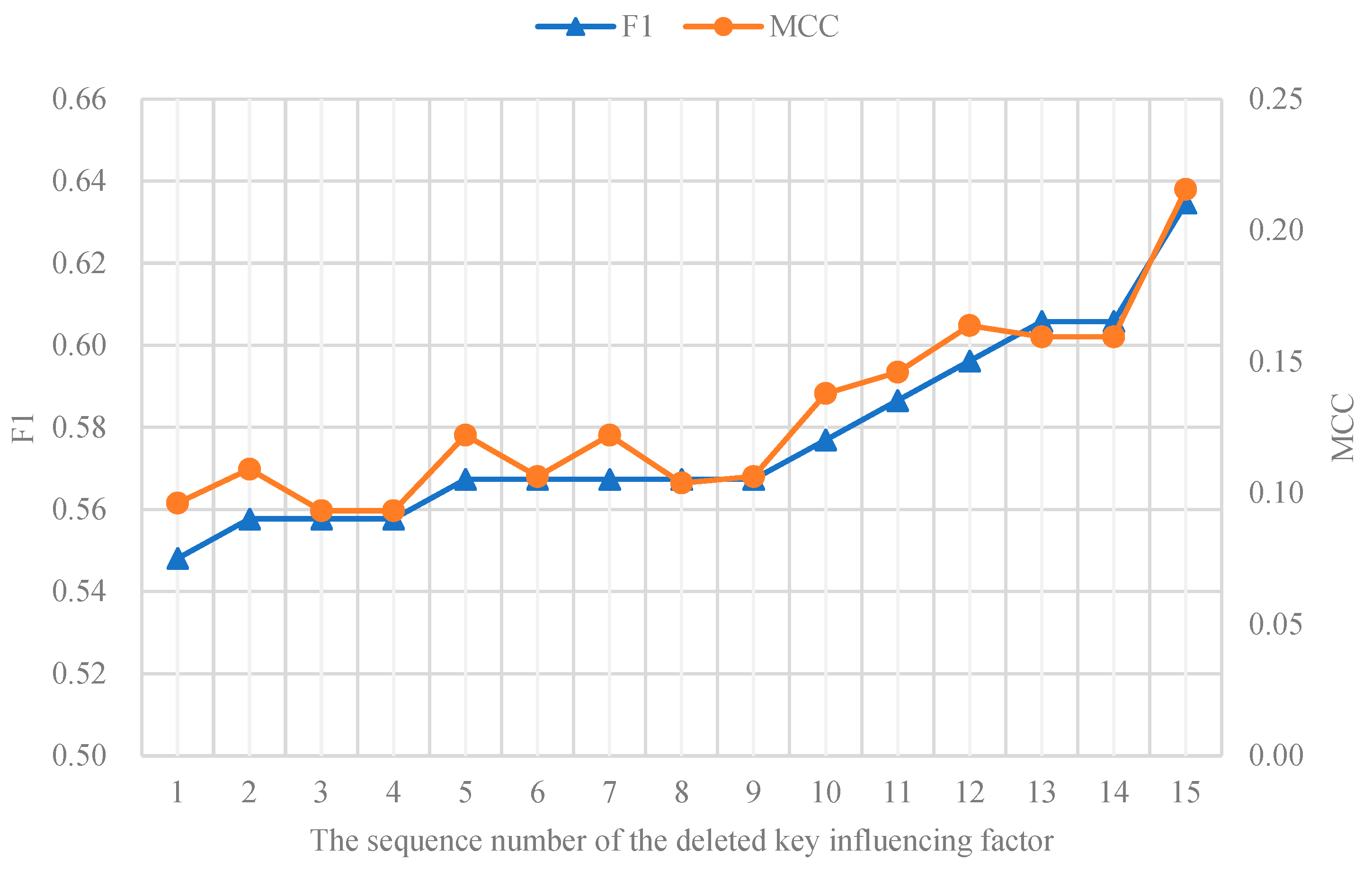
For the pre-processed experimental dataset, we set 1/4 of them as the test group and the rest as the training group. A common logistic regression classifier was adopted as the classifier used in the experiment. When we took all 448 feature variables as the input of the classifier, we obtained F1 and MCC values of 0.4216 and 0.0612, respectively. When we took the selected 15 key influencing factors as the input of the classifier, the values of F1 and MCC were 0.6431 and 0.2209, respectively. On this basis, we sorted key influencing factors according to their importance, deleted the first to 15th key influencing factors, and took the remaining key influencing factors as the input of the classifier to obtain the corresponding F1 and MCC evaluation index values. The experimental results are shown in Figure 8.

In Figure 8, N = 1 indicates that the first key influencing factor is deleted, and the remaining 14 key influencing factors are used as characteristic variables. In this case, the obtained F1 value and MCC value are 0.548 and 0.096, respectively. N = 2 means that the second key influencing factor is deleted and the other remaining 14 key influencing factors are used as characteristic variables.

5. Discussion

Figure 6 shows that among the 15 key influencing factors, three are the direct causes of the target variable, and 10 are included in the second-order local causal network of the target variable. Among them, the three direct causes of the target variable have a great impact on the causal pathway pointing to the target variable in the global causal network, and the normalized causal pathway contribution degree is 19.97%, 18.60%, and 7.11%, respectively, which also indicates that the direct cause node on the Markov blanket has a decisive impact on its corresponding target variable.

In combination with Figure 5 and Figure 6, we can also conclude that some indirect causes also have higher causal pathway contribution degrees to the target variable, and a few indirect causes have greater causal pathway contribution degrees to the target variable than other direct causes. For example, the two indirect causes numbered 215 and 95 have a higher causal pathway contribution degree to the target variable than the three direct causes numbered 55, 106 and 277. Among them, the normalized causal pathway contribution degree of node 215 is 11.86%, and the normalized causal pathway contribution degree of node 95 is 11.49%.

By comparing Figure 6 and Figure 7, we see that when only the number of causal pathways is considered, the key factors influencing the target variable are basically consistent with those when the number of causal pathways and the length of causal pathways are considered simultaneously. In both results, only one factor changed: Node No. 72, which ranked 15th in Figure 6, was changed to Node No. 4, which ranked 15th in Figure 7. However, the ranking of key influencing factors in the two results changed significantly: Only the ranking of node 51 in the 8th ranking and node 6 in the 13th ranking remain unchanged. Considering that the influence of the cause variable on the target variable gradually decreases with the length growth of the causal pathway, it is more scientific to calculate the contribution degree of the causal pathway by comprehensively considering the number of causal pathways and the length of causal pathways.

From the experimental results in Section 4.6, when all characteristic variables are taken as inputs to the classifier, the prediction performance of the classifier is relatively poor, and F1 = 0.4216 and MCC = 0.0612. When we use the selected 15 key influencing factors as characteristic variables, the prediction performance of the classifier is greatly improved, and F1 = 0.6431 and MCC = 0.2209. This also confirms the theoretical basis of feature selection: For a given sample size, there is a maximum number of features above which the performance of our classifier degrades rather than improves in most cases, and the additional information that is lost by discarding some features is (more than) compensated by a more accurate mapping in the lower-dimensional space. As seen from Figure 8, when we successively delete the key influencing factors ranked 1–15 and take the remaining 14 key influencing factors as the feature variables, the prediction performance of the classifier is gradually improved—the values of F1 and MCC both gradually increase. This also shows from another aspect that there are indeed differences in the specific impacts of the selected key influencing factors on the system. The higher the ranking of key influencing factors is, the greater the corresponding impact on the system.

In general, simulation experiments based on the SECOM dataset obtained causal networks among variables that drive the dataset generation. Based on the heuristic causal inference method proposed in this paper, several factors that have a key impact on product quality were identified. This achievement has a certain guiding significance for understanding the monitoring data in semiconductor production. In an ideal situation, the overall operation of the production line can be determined by analysing the monitoring data corresponding to the direct cause of the target variable. When the monitoring data of some direct causes cannot be obtained, the analysis of the monitoring data corresponding to the key indirect causes can also be meaningful. For the craftsmen on the production line, the targeted operation and maintenance guarantee according to the key influencing factors can reduce the unit production cost and improve the overall efficiency of the system.

6. Conclusions

In view of the natural advantages of causal inference in revealing the essential laws of things, a heuristic causal inference method for identifying the key factors influencing complex systems is proposed. On the basis of acquiring the causal network among variables by using observational data, the direct cause and indirect cause of the target variable are defined, and the global causal pathway, local causal pathway, and average causal pathway length from the cause variable to the target variable are defined. By referring to the analysis approach for a complex network, the causal pathway contribution degree is proposed to replace the causal effect of the cause variable on the target variable. Based on this, heuristic causal inference is carried out, which helps to quickly identify the key factors influencing the system from the perspective of causality.

Simulation experiments are carried out on the SECOM dataset, and a causal network consisting of 347 nodes and 493 edges is obtained. Taking product quality test results as the target variable, the key influencing factors are identified. Based on the modelling analysis process and the experimental results of our research, the following conclusions can be drawn:

(1) It is feasible to analyse complex systems via causal science, and the causal network that drives the generation of a system monitoring dataset can be obtained by combining the traditional causal discovery method with domain prior knowledge.

(2) The heuristic causal inference method proposed in this paper addresses the problem that it is difficult to identify key influencing factors in complex systems. The core index of heuristic causal inference, the causal path contribution degree, can scientifically reflect the causal impact of cause variables on the target variable and can be quantitatively calculated with low computational complexity.

(3) Compared with the method based on experimental simulation and DEMATEL, our proposed method has certain advantages. First, our proposed method does not need to establish a system simulation model, so it has better applicability. In general, it is expensive or impossible to build simulation models for complex systems with multiple factors. In addition, the proposed method combines the theories and techniques of network science and causal science and is based on the scientific analysis of data generated by complex systems, avoiding the influence of experts’ subjective factors, such as the DEMATEL method, on the analysis results to have a higher degree of availability.

Since the proposed model combines the theory of causal inference and complex networks, it can be used to analyse complex systems and problems in different forms in practical applications, such as the analysis of the causes of major diseases and the analysis of the key factors affecting education. Since we made only a preliminary exploration, we can continue to conduct in-depth integration studies of complex networks and causal inference in the future, including considering causal factors in network topology analysis and studying robustness and evolution rules in causal networks.