Integrating Hourly Scale Hydrological Modeling and Remote Sensing Data for Flood Simulation and Hydrological Analysis in a Coastal Watershed

Featured Application

Application of the SWAT model at an hourly scale for flood simulation in a coastal basin.

Abstract

Hourly scale hydrological modeling holds pivotal significance for flood-related research, as watershed floods often occur within a few hours of intense rainfall. Although the SWAT model’s hourly simulation has found application in a few watersheds, the relatively short usage history and limited scope inhibit a comprehensive grasp of its potential. In this study, a coastal watershed in Fukuyama City, Japan was selected as a case study for conducting hourly simulations. The study highlights the hourly simulation’s proficiency in capturing diverse flood trends while also accurately replicating baseflow and flood peaks within the 0 to 200 m³/s range. However, there is an underestimation of peak flows in calculations exceeding 200 m³/s. Moreover, empirical summaries have been generated to outline the parameterization process of hourly simulation, revealing how distinct parameters influence simulated runoff. For instance, it outlines how BFLO_DIST significantly affects baseflow simulation when operating in hourly mode. Our findings provide an empirical summary of the advantages, disadvantages, and parameterization process for hourly simulations of the SWAT model.

1. Introduction

The occurrence of flooding stands as a substantial natural catastrophe, posing a severe peril to human communities and profoundly affecting both lives and property safety. Concurrently, as global temperatures have continued to rise in recent decades, an upsurge in anomalous climatic events, including floods triggered by unprecedented rainstorms, has been observed [1,2,3]. The global natural disasters recorded by the Emergency Events Database (EM-DAT) include a total of 14,581 natural disaster events from 1900 to 2018 worldwide, within which flood events account for the highest proportion of 33% [4].

The Soil and Water Assessment Tool (SWAT) model, developed by the US Department of Agriculture in 1995, was constructed on the basis of the Simulator for Water Resources in Rural Basins (SWRRB) model [5]. During nearly three decades of development, eight distinct versions of the model have been introduced [6,7]. What initially began as the SWAT/GRASS interface has since evolved into the AVSWAT and ArcSWAT interfaces [8]. The initial SWAT model began as computer code and was later evolved into a version integrated with a Geographic Information System (GIS) interface. This integration facilitated easy data processing and model visualization. Furthermore, it simplified the linkage to sensitivity, calibration, and uncertainty analysis tools, such as SWAT-CUP. Throughout the development of the interface, continuous improvements were made to enhance its functionality, resulting in its widespread recognition and application. Initially designed for evaluating hydrological, sediment, and water quality conditions in watersheds, the SWAT model is now primarily employed for hydrology, sedimentation, crop growth, nutrient cycling, and management of pest hazards. Sinnathamby et al. [9] adjusted crop module parameters for corn and sorghum within the SWAT framework and obtained improvements in modelling results. Mekonnen et al. [10] incorporated seasonally varying soil erodibility into the SWAT model, and they effectively simulated daily nutrient export in a cold prairie watershed in Canada. Additionally, Zhang et al. [11] examined the effects of almond pest management practices on water quality in California, USA, and their study revealed that almond pesticide usage had a significant impact on pesticide loads within the San Joaquin River watershed.

The capability of adapting to different infiltration procedures on varying time scales enables the SWAT model to simulate on various time scales, including annual, monthly, daily, hourly, and even minute-long intervals [12]. Singh and colleagues [13] adeptly utilized the SWAT model to replicate runoff at both daily and monthly scales for the Tungabhadra watershed, illuminating a robust correlation between observed and simulated values. Additionally, Meng et al. [14,15] leveraged the China Meteorological Assimilation Driving Datasets (CMADS) meteorological dataset in conjunction with the SWAT model to scrutinize significant watersheds in China across diverse temporal contexts, successfully meeting model evaluation criteria through correlation coefficient (R²) and Nash–Sutcliffe model efficiency coefficient (NSE) assessments. Nonetheless, the heightened temporal granularity intrinsic to hourly simulations might lead to a relatively reduced accuracy when contrasted with daily simulations. In-depth analysis of hourly scale simulation outcomes by Bauwe and colleagues involved the application of the SWAT model’s Green–Ampt methodology to scrutinize the impact of hourly precipitation resolution on model performance and hydrological attributes [16]. Furthermore, Campbell and co-authors [17] harnessed the SWAT model at an hourly scale for the Pawtuxet Watershed. However, the NSE results, falling below anticipated levels, underscored important insights for both the calibration and validation phases.

Jeong and colleagues [18] introduced the innovative hourly simulation module of the SWAT model in 2010. SWAT provides two methods for estimating surface runoff: the Soil Conservation Service (SCS) Curve Number (CN) method and the physically based Green and Ampt Mein Larson (GAML) method. The GAML method could be implemented in hourly simulations to continuously simulate the infiltration processes. The GAML equation establishes a relationship between the infiltration and rainfall rates based on parameters with physical meanings, facilitating the continuous simulation of surface runoff [18]. Therefore, the SWAT model could be implemented at an hourly scale, and the high-resolution time interval is critical for accurately modeling watershed floods. Given its relatively recent inception, scarcity of established simulation methodologies, and increased uncertainties, the application of the SWAT model at hourly scales for watershed studies remains less prevalent. In an example among the limited published investigations, Yang and co-authors [19] performed a comparative analysis contrasting flow simulations between hourly and daily scales, revealing substantial impacts of different temporal resolutions on the hydrological processes. Recognizing the daily scale’s limitations in capturing intricate temporal nuances of river flow and material dynamics, Shannak [20] extended efforts to reinforce the predictive capabilities of the hourly scale model, specifically concerning high-resolution flood peak forecasts. Furthermore, Boithias and collaborators [21] employed the hourly module for predicting flow in coastal watersheds. However, hourly simulated R² and NSE values showcased subpar performance across various stations in contrast to daily scale simulations.

While the application and performance of SWAT models with various time resolutions have been discussed in previous studies, a lack of comprehensive evaluations addressing the intricacies of hourly scale simulated flood peaks persists, encompassing their advantages, disadvantages, and the involved parameterization procedures. Therefore, the objectives of this study are: (a) to establish a reliable SWAT model to shed light on the advantages and disadvantages of the model in flood peak and baseflow simulations at different scales; (b) to investigate the sensitivity of the simulated hourly runoff to different parameters; and (c) to explore the intra-annual dynamics of hydrological components in the basin, providing fundamental information for water resource management.

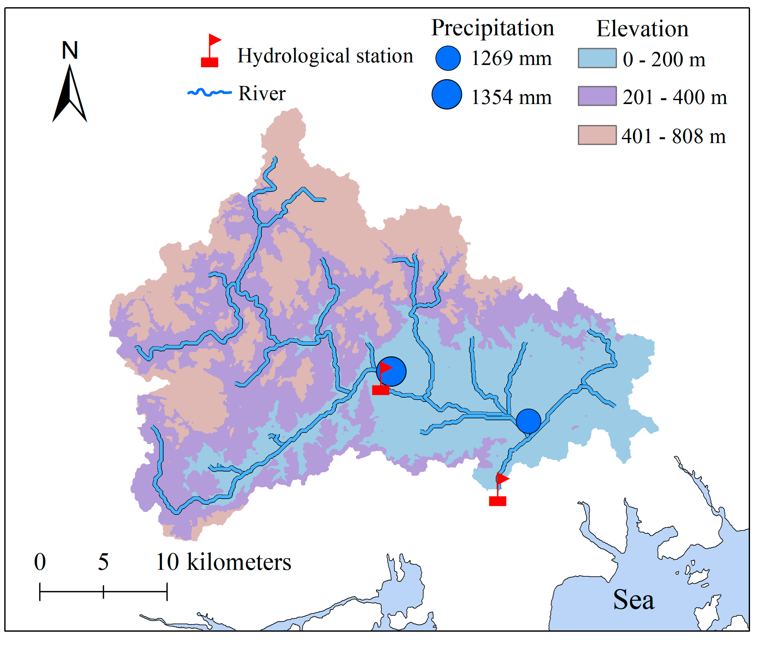
2. Study Sites and Materials

The study area chosen is situated within the confines of Fukuyama City. Due to its geographical location and steep topography, the study basin is susceptible to flood. Meanwhile, the hydrometeorological indexes are well monitored using two meteorological and hydrological stations, and the high quality of the observational data makes the model’s simulation results more reliable. The Ashida River ranks as the third longest river within Hiroshima’s boundaries. The river flows from the northwest to the southeast, meandering through Fukuyama City before eventually merging with the Seto Inland Sea (as depicted in Figure 1). The large urban areas within the basin form a high proportion of impervious surface, which reduces the soil’s infiltration capacity and results in rapid runoff accumulation, leading to more frequent and intense floods. Nestled within the subtropical monsoon zone, the watershed experiences an average annual temperature of approximately 16.0 °C. The basin has an average annual precipitation of 1814 mm, equivalent to a yearly water volume of 1.39 km³. Large precipitation amounts and high-intensity rainfall events have the potential to damage the basin’s water storage projects, increasing its vulnerability to flood. Notably, the average runoff at the river mouth during the year 2017 stood at approximately 17.5 m³/s. Encompassing an extensive expanse of 759.5 km² (with coordinates ranging from 34.46° N to 34.71° N and 133.02° E to 133.43° E), the watershed encompasses an urban area spanning 77.5 km², while the forested domain occupies approximately 562.8 km². Fukuyama City has an estimated population of approximately 460,000 residents. Topographically, the area features elevated terrain in the west and north, gradually giving way to lower terrain in the east and south. Mountains and hills are mainly distributed in the northwest, and plains are mainly distributed in the east. The elevation in the basin ranges from 3 m to 720 m. Mountains and hills are mainly distributed in the northwest, and plains are mainly located in the east of the basin. The topographic pattern promotes fast runoff flow in the upstream reaches and relatively slow runoff flow in the downstream reaches. The study includes two carefully selected hydrographic stations: the Fuzhong Station, strategically located upstream of the Ashida River’s entry into the city, and the Shanshou Station, strategically positioned prior to the river’s merging point with the sea.

Building the SWAT model database hinges on pivotal datasets, namely Digital Elevation Model (DEM) data, soil data, land use data, and meteorological data (refer to Figure 2 for the depiction of watershed conditions). The study area’s DEM data were sourced from the U.S. Geological Survey website. The Terra Advanced Spaceborne Thermal Emission and Reflection Radiometer (ASTER) Global Digital Elevation Model (GDEM) Version 3 (ASTGTM) provides a global DEM of land areas on Earth at a spatial resolution of 1 arc second (approximately 30 m horizontal posting at the equator). Chaubey et al. [22] demonstrated that the accuracy of the 30 m resolution elevation data-driven SWAT model simulation is higher than that of the simulation results with lower resolution data. The ASTGTM data product was created by automating the processing of the entire ASTER Level 1A scenario archive acquired between 1 March 2000 and 30 November 2013. The data product was cleansed of residuals and outliers, and it was presented in a raster format. The land use classification was derived from the secondary grid classification of SPOT and RapidEye remote sensing images by the Japanese Land Agency, and the image year used was 2016, which is very close to our study year. The data format was shape. Soil classification was derived from field surveys of physical and chemical soil properties conducted by the Japanese Land Agency across the country. The data format was shape. Meteorological and hydrological data were derived from observatories belonging to the Japanese government. The runoff (m³/s), precipitation (mm), air temperature (°C), wind speed (m/s), solar radiation (MJ/m²), and relative humidity (%) required by the model were all measured by the automatic observation instrument of the observation station. The original data downloaded were in .xls format.

Table 1. The description of the data sources for SWAT hourly simulation.

Data Type	Source URL	Resolution/Scale/Number of Sites
DEM	https://earthexplorer.usgs.gov (19 July 2019)	30 m
Soil	https://nlftp.mlit.go.jp (29 July 2019)	1:1,000,000
Land use	https://nlftp.mlit.go.jp (29 July 2019)	1:25,000
Weather	http://www.data.jma.go.jp (30 July 2019)	2
Hourly river flow	http://www.river.go.jp (5 August 2019)	2

provides comprehensive information on the utilized data.

3. Methodology

The SWAT model’s computational framework has been continuously enhanced and refined since 1995, progressively expanding its applicability due to the model’s powerful computational capabilities and robust physical mechanisms. Consequently, it has become a pivotal foundation for developing strategies and policies in managing water resources [23,24]. According to a 2015 statistical study on hydrological modeling [25], the SWAT model was employed in about 46% of such studies, indicating its position as one of the most widely used hydrological models. In the model’s temporal scope, the recent inclusion of the SWAT model’s hourly simulation module introduces greater complexity. However, it necessitates heightened precision in meteorological input data, real measurements, and a higher level of intricacy compared to daily scale simulations [26].

DEM input data are used to delineate watershed boundaries, define sub-basins, establish the river network, and generate flow directions in the watershed. Once the watershed information is extracted, land use and soil property data are incorporated into the model. Topography, land use, and soil property data are reclassified, and unique combinations of land use type, soil type, and slope type are categorized as Hydrologic Response Units (HRUs) in the SWAT model. It assumes that HRUs within the same class exhibit similar hydrological behaviors, and hydrological processes are computed separately for each class of HRUs in sub-basins. Meteorological information for each HRU is generated based on the data from the nearest meteorological station.

This study utilized ArcSWAT version 2012 to build the model and performed parameterization using SWAT-CUP 2012. The watershed extraction function within ArcSWAT 2012 was utilized to delineate sub-basins and establish river networks. ArcSWAT 2012 automatically extracts sub-basins and establishes river networks based on the elevation data, and it determines the number of sub-basins and the density of river networks by setting the minimum area threshold of sub-basins. The principle is that it should be detailed enough to capture significant topographic changes within the watershed. In this study, we divided a basin of 759.5 km² into 47 sub-basins, which is a relatively detailed division, although the sub-basin division levels basically do not clearly affect the simulation results [27]. In addition, we used Google Earth to verify the river network path automatically extracted by the model to prevent path deviation. A threshold of 981 ha was adopted for watershed extraction, leading to the classification of 369 hydrological response units. Precipitation data with a 1 h interval were input into the model, formatted as “year month day, 60” with “60” signifying 60 min (equivalent to 1 h). The calibration and validation of the SWAT model were executed using the SUFI-2 algorithm within the SWAT-CUP software. Throughout this process, hourly runoff measurements were incorporated in the format “FLOW_OUT_Year_Month_Day_Hourly Runoff Value”. In contrast to daily, monthly, and annual scale simulations, the inclusion of an hourly simulation plug-in was essential for executing hourly simulations. Since the original SWAT-CUP software only works on daily, monthly, and yearly scales, a plug-in for hourly simulation was designed for calibration and extraction in SWAT-CUP. To use the hourly plug-in for this study basin, it was necessary to adjust the river outlet name in the “fig.fig” file and the number of simulated stations, sub-basin numbers, and simulation year in the “SUFI2_extract_rch_hrly.def” file.

The SWAT-CUP uses a multiple regression approach to quantify the sensitivity of each parameter:

$$\mathrm{g}=\propto +{\displaystyle \sum }_{\mathrm{i}=1}^{\mathrm{n}}{\mathsf{\beta }}_{\mathrm{i}}{\mathrm{b}}_{\mathrm{i}}$$

where g is the objective function value, α is the regression constant, and β is the coefficient of parameters. The T-stat was then used as a way to identify the relative significance of each parameter b [28]. The sensitivities provided above are estimations of how the objective function changes on average when each parameter is altered, while all other parameters are in a state of flux. These estimations yield relative sensitivities based on linear approximations. The p-value determines the significance of the sensitivity. The SUFI-2 method employs Latin Hypercube sampling to manage parameters, and the calculation steps can be outlined as follows: first, define an objective function. Then, in the initial round of Latin Hypercube sampling, allocate sampling points within the initial parameter uncertainty range. Next, move on to subsequent rounds of Latin Hypercube sampling, calculating a series of measurement matrices to evaluate each sampling point. Finally, based on the evaluation results, proceed to update the parameter ranges further.

4. Results

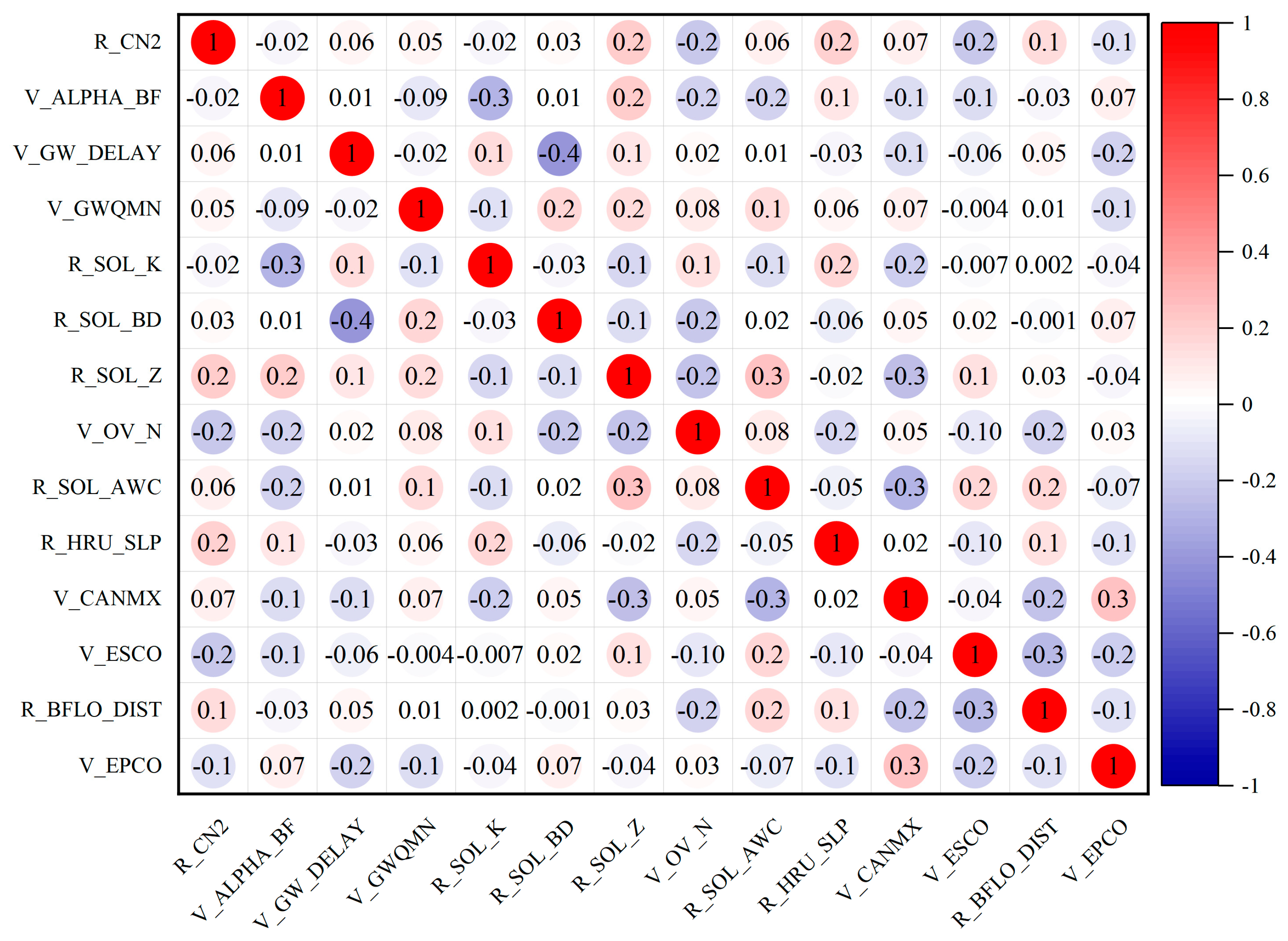
4.1. Parameter Sensitivity

SWAT-CUP covers a wide range of model parameter attributes, including groundwater characteristics, soil properties, vegetation attributes, hydrologic response unit factors, management settings, and channel attributes. The pursuit of credible and dependable parameters from this extensive array is the driving force behind parameter sensitivity analysis. This analysis serves a dual purpose, refining not only the parameter selection process but also enhancing comprehension of the roles these parameters play in watershed simulation. Ultimately, this process allows for a concentrated effort to fine-tune the more sensitive parameters, thereby aligning simulated values more closely with observed counterparts.

4.1.1. Global Sensitivity

The test-statistic (T-stat) was introduced by statistician Student in 1908 [29]. It is a valid statistical test that can be used to test whether the difference between two samples is significant. The p-value offers an alternative to traditional rejection thresholds, providing the smallest level of significance at which one would reject the null hypothesis. A smaller p-value indicates stronger evidence in favor of the alternative hypothesis. T-stat and p-value are employed as metrics to evaluate the sensitivity of model parameters. A widely held perspective is that a parameter exhibits greater sensitivity when its T-stat’s absolute value is larger and its p-value approaches zero. In contrast, parameters are considered less sensitive if their T-stat’s absolute value is smaller and their p-value is larger. The sensitivity ranking of each parameter during the calibration period provides guidance for the next calibration, and the parameters with high sensitivity become the primary target of the next adjustment. The range of parameters with high sensitivity is adjusted to see if the simulated values agree with the observed values. However, the adjustment of parameters with low sensitivity will have little or no effect on the change of the simulated value. After determining the parameter range during the calibration period, we used the same parameter range to simulate the runoff in the validation period. In this process, NSE and R² values were used to determine whether the simulated runoff was consistent with the observed runoff in the validation period [30,31]. If the NSE and R² values do not meet the evaluation criteria (NSE > 0.5, R² > 0.5), the parameters with high sensitivity are adjusted again until the results for both the calibration and validation period are satisfactory. The statistical data presented in

Table 2. Parameter calibration results and sensitivity analysis ranking.

ID	Parameter Name	Description	T-Stat	p-Value	Fitted Value	Min Value	Max Value
1	SOL_BD	Moist bulk density (Mg/cm3)	5.66	0.00	0.37	0.30	0.50
2	ALPHA_BF *	Baseflow alpha factor (days)	−4.11	0.00	0.04	0.00	0.20
3	BFLO_DIST	Baseflow distribution factor for sub-daily simulation (fraction)	−3.53	0.00	−0.97	−1.00	−0.90
4	CN2	SCS runoff curve number (dimensionless)	−3.00	0.00	0.01	0.00	0.10
5	ESCO *	Soil evaporation compensation factor (fraction)	−1.37	0.18	0.98	0.90	1.00
6	SOL_AWC	Available water capacity of the soil layer (fraction)	1.19	0.24	−0.66	−0.70	−0.60
7	GWQMN *	Threshold depth of water in the shallow aquifer required for return flow to occur (mm)	1.07	0.29	304.00	100.00	500.00
8	OV_N *	Manning’s “n” value for overland flow (dimensionless)	1.00	0.32	23.0	20.00	23.00
9	EPCO *	Plant uptake compensation factor (fraction)	0.70	0.49	0.80	0.60	0.90
10	CANMX *	Maximum canopy storage (mm)	−0.70	0.49	5.82	5.00	7.00
11	HRU_SLP	Average slope steepness (m/m)	−0.37	0.72	−0.80	−0.80	−0.70
12	SOL_Z	Depth from soil surface to bottom of layer (mm)	0.36	0.72	−0.48	−0.60	−0.20
13	SOL_K	Saturated hydraulic conductivity (mm/hr)	−0.14	0.89	2.13	1.80	2.50
14	GW_DELAY *	Groundwater delay (days)	0.10	0.92	0.75	0.00	3.00

Note. The symbol “*” indicates that the parameter value is to be replaced by a given value.

outline the sensitivity ranking of parameters during the calibration period, along with their corresponding fitted values, range values, and properties. Presenting properties information for parameters allows readers with limited knowledge of hydrological models to more easily grasp the meaning of the parameters. Additionally, attribute descriptions for parameters facilitate the identification of their respective categories (such as groundwater, soil, hydrological response units, etc.), thereby aiding in the comprehension of the hydrological processes within the watershed model.

Parameters with T-stat absolute values exceeding 3 include soil moist bulk density (SOL_BD), baseflow alpha factor (ALPHA_BF), and baseflow distribution factor for subdaily simulation (BFLO_DIST). Among these, soil moist bulk density emerges as the most influential parameter for hourly runoff simulation. A higher value of soil moist bulk density signifies an augmented likelihood of surface water percolating through the soil as lateral flow and groundwater, consequently curbing basin evaporation. BFLO_DIST, a parameter tailored for hourly simulations, represents an hourly scale baseflow distribution coefficient pivotal in governing baseflow values for such simulations. Its modulation mechanism dictates that a smaller value fosters a more even distribution of river baseflow within each hourly step over the course of a day, while a larger value introduces heightened variability. When the simulated baseflow value falls short of the observed value, appropriate adjustments to the BFLO_DIST parameter can effectively optimize simulated outcomes in alignment with the basin’s actual characteristics. Sensitivity ranking serves as a valuable indicator for enhancing calibration efficiency. This is evident during the subsequent calibration process, where we prioritize parameters with high sensitivity and deemphasize the adjustment of parameters with low sensitivity. According to the findings presented in Table 2, we can conclude that certain parameters, like GW_DELAY, exhibit limited sensitivity to the simulation’s impact. Consequently, they do not warrant a high priority in the subsequent parameter range adjustment process.

Figure 3 displays the distribution of 14 parameter values and NSE values in a global sensitivity analysis. By analyzing the linear relationship between the distribution of each parameter and the simulation effect (NSE), this provides suggestions for adjusting the parameter range. The positive correlation between the parameter distribution and the simulation effect indicates that increasing the maximum or minimum value of the parameter may be conducive to improving the simulation effect, while the negative correlation between the parameter distribution and the simulation effect indicates that decreasing the maximum or minimum value may be conducive to improving the simulation effect. Parameters exhibiting a negative linear relationship include CN2, ALPHA_BF, GW_DELAY, SOL_Z, HRU_SLP, and BFLO_DIST. Conversely, other parameters demonstrate a positive correlation. The degree of scatter dispersion is linked to parameter sensitivity, with highly sensitive parameters showing more clustered scatter plots, such as SOL_BD and ALPHA_BF. For these parameters, the scattered points predominantly cluster within the 0.5–0.6 interval of NSE, indicating that the parameter range we ultimately selected closely aligns with the optimal range following multiple calibration efforts.

Interactions and influences among parameters within the SWAT model may introduce potential sources of unreliability in sensitivity analysis results. Consequently, we carried out a correlation analysis on the simulated parameter values (Figure 4). Notably, significant correlations were observed among certain parameters; for instance, the correlation coefficient between SOL_BD and GW_DELAY was found to be −0.4, the correlation coefficient between SOL_K and ALPHA_BF stood at −0.3, and the correlation coefficient between SOL_AWC and SOL_Z reached 0.3. The correlations between parameters lead to parameter redundancy, which is part of model uncertainty. For its uncertainty, we performed another parametric sensitivity analysis, namely one-at-a-time sensitivity.

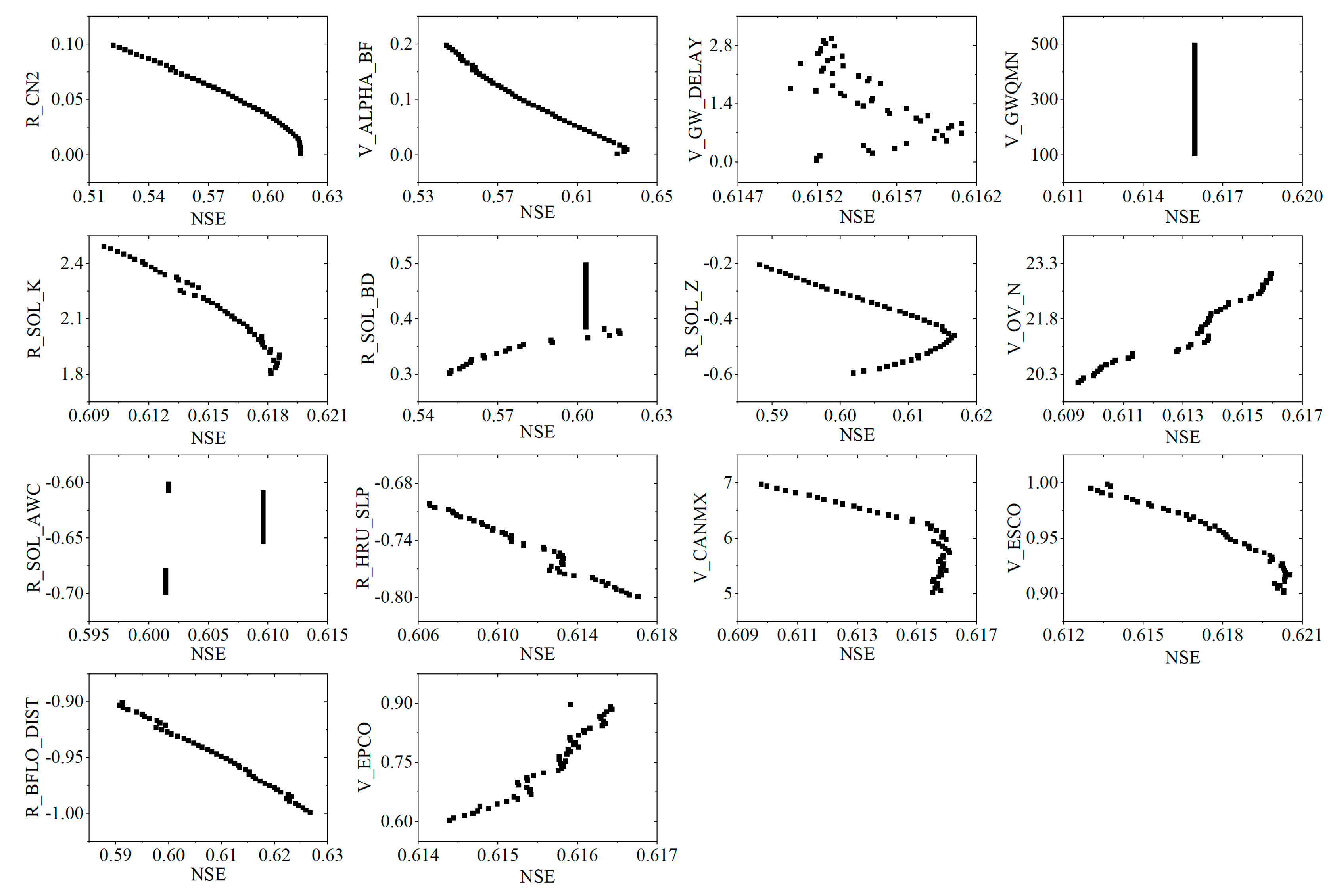
4.1.2. One-at-a-Time Sensitivity

One-at-a-time sensitivity, as a method, involves assessing the sensitivity of a single parameter by altering its value while keeping all other parameters constant. This method was proposed by Morris in 1991 and has a long history of application [32]. It enables a clear attribution of model output variations to specific parameter modifications. Consequently, the results are both quantitative and exclusive. In this analysis, the values of the other parameters were the fitted values established during the calibration period, while the altered parameter values spanned the parameter range established during that same calibration period, ranging from the minimum to the maximum values.

In one-at-a-time sensitivity (Figure 5), most of the parameters and simulation results show sensitivity except GWQMN. The smaller the values of CN2, ALPHA_BF, SOL_K, HRU_SLP, ESCO, and BFLO_DIST within the provided parameter range, the better the simulation effect. On the contrary, the values of OV_N and EPCO and the simulation effect show a positive trend in the range. The point distribution of relation between GW_DELAY and NSE is discrete, which is consistent with the low sensitivity in our global sensitivity analysis. We have noticed that the change of GWQMN value does not affect the value of NSE, but its T-stat value is greater than 1 in global sensitivity. The high sensitivity of GWQMN in global sensitivity may be a false phenomenon caused by the influence of the SOL_BD parameter (Figure 4). In addition, we also noticed that the fitted value of one-at-a-time sensitivity analysis was close to the fitted value of global sensitivity simulation, which provided credible evidence for the results of calibration.

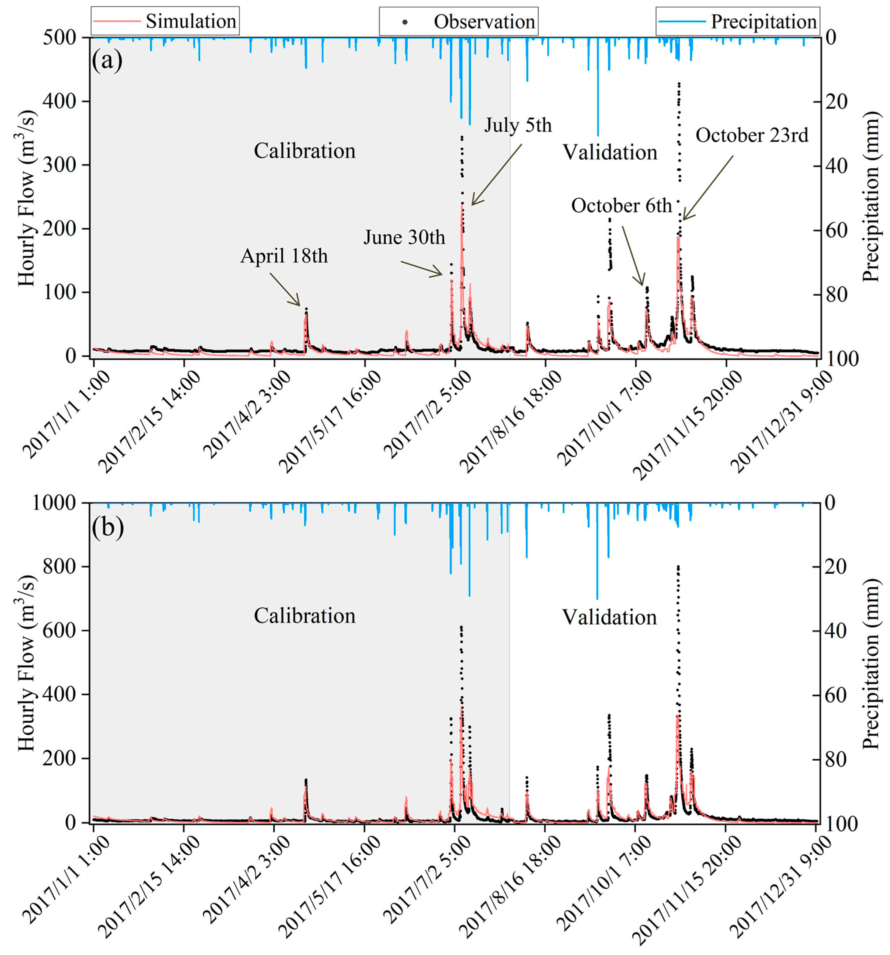
4.2. Runoff Simulation

The Ashida River basin experienced its most intense precipitation in July and October 2017, with the peak hourly flow rate reaching 800.5 m³/s in that year at the Shanshou Station. The selected study timeframe spans from 0:00 a.m. on 1 January to 23:00 p.m. on 31 December 2017. The calibration period encompasses from 0:00 a.m. on 1 January to 23:00 p.m. on 31 July, while the validation period spans from 0:00 a.m. on 1 August to 23:00 p.m. on 31 December. The hourly runoff simulations conducted throughout the study period are illustrated in Figure 6. Notably, these simulations effectively capture the variations in runoff characteristics during both flood and non-flood periods at the two designated stations. Evaluating the simulation results using corresponding performance indices R² and NSE, as presented in

Table 3. Evaluation of hourly flow simulation results at Fuzhong Station and Shanshou Station.

Index	Fuzhong Station		Shanshou Station
	Calibration	Validation	Calibration	Validation
R2	0.64	0.61	0.65	0.56
NSE	0.61	0.59	0.64	0.57

, both indices surpass 0.55 overall. Furthermore, during the calibration period, both R² and NSE surpass 0.6, showcasing the model’s favorable performance during this specific interval.

The figure reveals that the hourly simulations exhibit greater accuracy for moderate peak flows and baseflow (ranging from 0 to 200 m³/s), aligning closely with observed runoff values. Notable instances include 18 April (74.3 m³/s simulated vs. 64.0 m³/s observed), 30 June (143.9 m³/s simulated vs. 120.0 m³/s observed), and 6 October (107.4 m³/s simulated vs. 71.6 m³/s observed). While the metrics suggest a higher level of satisfaction with the SWAT model’s hourly scale simulations, it is evident that a significant portion of high peak flow (>200 m³/s) simulation results still underestimate the observed runoff peaks. For example, 5 July (343.8 m³/s simulated vs. 238.0 m³/s observed) and 23 October (427.7 m³/s simulated vs. 186.0 m³/s observed) stand as instances where underestimation is pronounced. This phenomenon can be attributed to two factors. Firstly, the two employed meteorological stations may not have effectively and comprehensively captured the extremities of high precipitation events. Secondly, the occurrence of extreme heavy rainfall events can trigger both natural and human-induced anomalies in river runoff (e.g., minor weir breaches, reservoir discharges, etc.). Given the fine temporal resolution of hourly simulations, their capacity to accommodate such aberrations is comparatively limited in comparison to daily scale simulations. Consequently, the hourly scale simulations demonstrate relatively less proficiency in accurately reproducing peak flows during instances of exceptionally high discharge.

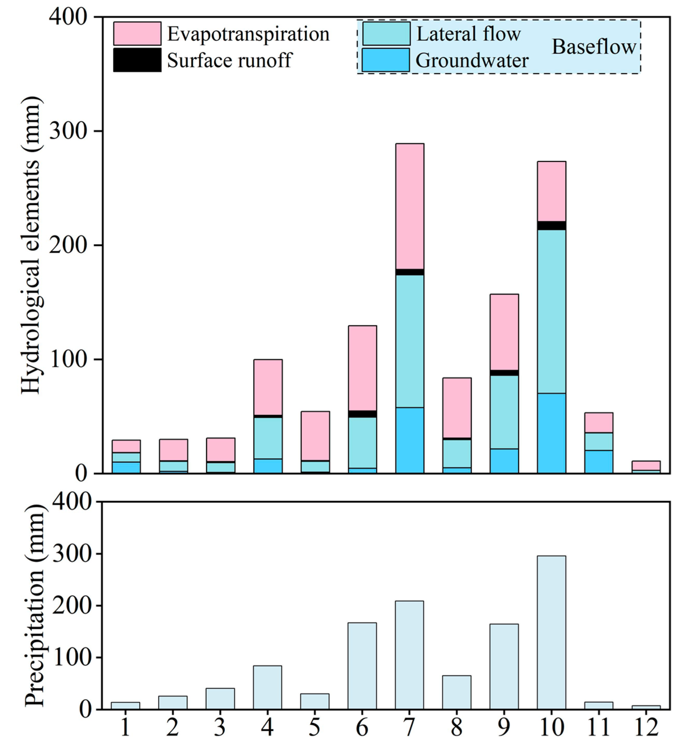
4.3. Hydrological Elements

The model outcomes were employed to scrutinize the intra-annual fluctuations of major hydrological constituents within the basin (refer to Figure 7). The findings reveal that variations in hydrological components—comprising surface runoff, lateral flow recharge to runoff, and groundwater recharge to runoff—generally mirror the oscillations in precipitation. When precipitation peaked in April, July, and October, these hydrological components also peaked in those months. The largest increase in precipitation was 449% in June compared to May. During this period, surface runoff, lateral flow recharge to runoff, and groundwater recharge to runoff increased by 828%, 371%, and 287%, respectively. The largest decrease in precipitation was a −95% change from November to October. The surface runoff, lateral flow recharge to runoff, and groundwater recharge to runoff changed by −95%, −89%, and −72%, respectively. The magnitude of change in these hydrological components differed from the magnitude of change in precipitation, but the trend of change (increase or decrease) was consistent. However, noteworthy temporal disparities emerge, with groundwater changes lagging behind shifts in surface runoff and lateral flow recharge to runoff. Groundwater recharging rivers encounters obstacles, such as rocks, soils, and other geologic materials, that cause it to flow at a slower rate. The sluggish response of groundwater may be related to local geologic and topographic conditions. Even though November’s precipitation falls below 15 mm, groundwater recharge to runoff registers at 20 mm. Due to the fact that in October, the precipitation reached a maximum of 295.7 mm among all the months of the year, a large amount of water was stored under the rocks as groundwater through soil infiltration, which was partly recharged to the runoff in the same month and partly flowed out in the following November due to the slow recharge of the groundwater. Furthermore, during months with equivalent precipitation (such as June and September), the recharge values of lateral flow and groundwater contributing to runoff were higher in September than in June. This difference can be attributed to the substantial summer precipitation (occurring in June, July, and August) being stored in aquifers, soil, and vegetation, which was subsequently released in September. Most of the rocks in the basin are igneous rocks (Figure 2), which are one of the hardest rocks, characterized by fewer unbreakable pores. The extensive prevalence of these rocks in the basin establishes favorable geological conditions for groundwater storage while simultaneously decelerating the rate of groundwater recharge. Furthermore, the watershed is predominantly covered by forests. During months with high precipitation, the trees’ roots, stems, and leaves have the capacity to store excess rainfall and gradually release it during dry periods. This process effectively maintains soil moisture content and enhances river runoff.

Cumulatively, across the entire year, basin-wide contributions from surface runoff, lateral flow to recharge, and groundwater to recharge represent 27.3 mm, 483.2 mm, and 205.0 mm, respectively. These figures correspond to 2%, 43%, and 18% of the total precipitation. The substantial presence of flow in the soil and groundwater suggests that water resources in this region easily infiltrate. This characteristic may be attributed to the prevalence of Dystric Regosol, a loose soil type distributed across numerous flat terrain areas within the basin. During the wet months (June–October), these three components account for 2.5%, 41.6%, and 14.9% of the precipitation, respectively. Conversely, in the dry months (January–May, November–December), these three components represent 2.1%, 47.7%, and 34.6% of the precipitation, respectively. This pattern reveals that as precipitation decreases, the proportion of surface runoff decreases, while the proportions of lateral flow to recharge and groundwater to recharge increase. Additionally, the annual basin-wide evapotranspiration in the region is 524.5 mm, accounting for 72.9% of the annual precipitation. Evapotranspiration, being the primary output of water quantity, is closely correlated with the vegetation cover and temperature of the basin. The significant contribution of evapotranspiration in this study area can be attributed to several factors. Firstly, the predominant land use in the area is forest, and forests have the capacity to retain water, making them a substantial source of water for transpiration by trees. Secondly, the high mean annual temperature, which averages at 16.0 °C, also plays a crucial role. In the intra-annual variation of evapotranspiration, although the precipitation in July is not the highest throughout the year, the evapotranspiration in this month is the highest (see Figure 7). This anomaly is primarily driven by the elevated temperatures in July, which lead to intensified water surface evaporation and plant transpiration.

Figure 8 illustrates the correlation between the principal hydrological components and precipitation for each of the 12 months. Each hydrological element has been tested for significance (

Table 4. The T-statistic and p-value for each hydrological element.

Elements	T-Statistic	p-Value
Surface runoff	3.25	<0.05
Lateral flow contribution to streamflow	3.03	<0.05
Groundwater contribution to streamflow	2.55	<0.05
Baseflow	2.91	<0.05
Evapotranspiration	4.95	<0.05
Air temperature	6.19	<0.05

). Correlation coefficients are established, revealing the associations between precipitation and various hydrological factors. Specifically, the correlation coefficients between precipitation and surface runoff, recharge of runoff through lateral flow, recharge of runoff through groundwater, and baseflow (lateral flow + groundwater) stand at 0.96, 0.92, 0.69, and 0.86, respectively. Notably, the correlation coefficient linking evapotranspiration and temperature (0.77) surpasses that of evapotranspiration and precipitation (0.57).

5. Discussion

The SWAT model has undergone optimization and development over the past two decades. However, as a model reliant on numerical computations, it is difficult to fully demonstrate the real and complex flow environment. Notably, the refinement of the SWAT model at an hourly scale remains a work in progress, with its practical application area yet to be comprehensively validated. It needs to pay special attention to the potential underestimation of flood peaks when using the SWAT model for hourly simulation and flood peak forecasting. To enhance the simulation accuracy, we recommend establishing a more extensive station network to obtain long-term hourly precipitation and hydrological observations in critical river basins. Furthermore, while the utilization of the SWAT model for water quality simulation at an hourly scale is currently limited, it holds significant promise for applications in water quality simulations at this temporal scale.

Examining the October 23rd flow instance in Figure 6 offers insight. Despite a flood peak of 800 m³/s occurring at 01:00 on that day, neither the Fuzhong nor the Fukuyama precipitation observatory registered an exceptionally large rainstorm. This disparity can be attributed to the vast watershed area and regional disparities in rainfall patterns. Such occurrences, wherein areas devoid of precipitation observations experience high-intensity rainfall, pose challenges to hourly simulations in accurately reflecting true flood peak values. Precipitation data, a pivotal input influencing runoff simulation within hydrological models, substantially shape the precision of the final flood simulation outcomes.

In some instances, the measured and simulated peak occurrences diverge by several hours. The two highest measured flood peaks lag behind their simulated counterparts by approximately 4 to 5 h. This temporal discrepancy arises from the influence of watershed topography on the timing of flow generation and convergence when precipitation transpires. The inherently uncertain nature of this process contributes to hourly simulated flood peaks, occasionally misaligning with actual peaks.

6. Conclusions

This study investigated the performance capability of the SWAT model in simulating runoff at the hourly scale, utilizing the coastal watershed as the subject of analysis. The research encompassed an assessment of the model’s effectiveness in capturing baseflow, moderate flood peaks (0–200 m³/s), and high flood peaks (>200 m³/s). Furthermore, the study explored sensitivities within 14 hydrologically significant parameters, elucidating their impacts on hourly simulations and offering insights to enhance the efficiency of high-temporal-scale simulations. An analysis of intra-annual variability of hydrological elements within the basin was conducted using the model. Consequently, several key conclusions emerged from the high-temporal-scale simulations conducted on the basin:

(a) The SWAT model’s hourly simulations largely succeeded in capturing variations in baseflow and moderate flood peaks (0–200 m³/s) at the hourly scale. However, underestimation was observed in simulating high flood peaks (>200 m³/s).

(b) In the parameter sensitivity analysis, specific parameters with significant impact on hourly flow simulations were identified, notably the influential role of the hourly simulation-specific parameter BIFO_LIST in regulating hourly scale baseflow.

(c) Through basin-wide hydrological element analysis, it was deduced that precipitation’s effects follow a descending order of magnitude on major hydrological constituents: surface runoff, lateral flow, groundwater, and evapotranspiration. Notably, the influence of precipitation on surface runoff surpasses its impact on baseflow.

References

1. Rudd, A.C.; Kay, A.L.; Sayers, P.B. Climate change impacts on flood peaks in Britain for a range of global mean surface temperature changes. J. Flood Risk Manag. 2023, 16, e12863. [Google Scholar] [CrossRef]
2. Veijalainen, N.; Lotsari, E.; Alho, P.; Vehvilainen, B.; Kayhko, J. National scale assessment of climate change impacts on flooding in Finland. J. Hydrol. 2010, 391, 333–350. [Google Scholar] [CrossRef]
3. Yang, G. Water issues in the Yangtze River and its formation causes and controlling strategies. Resour. Environ. Yangtze Basin 2012, 21, 821–830. [Google Scholar]
4. Wu, J.; Chen, F.; Chen, X. Temporal and spatial features and correlation studies of global natural disasters from 1900 to 2018. Resour. Environ. Yangtze Basin 2021, 30, 976–991. [Google Scholar]
5. Neitsch, S.L.; Arnold, J.G.; Kiniry, J.R. Soil and Water Assessment Tool User’s Manual; Version 2000; GSWRL Report 02-02; Grassland, Soil & Water Research Laboratory: Temple, TX, USA, 2002. [Google Scholar]
6. Arnold, J.G.; Srinivasan, R.; Muttiah, R.S.; Williams, J.R. Large area hydrologic modeling and assessment—Part I: Model development. J. Am. Water Resour. Assoc. 1998, 34, 73–89. [Google Scholar] [CrossRef]
7. Kannan, N.; Santhi, C.; Williams, J.R.; Arnold, J.G. Development of a continuous soil moisture accounting procedure for curve number methodology and its behaviour with different evapotranspiration methods. Hydrol. Process. 2008, 22, 2114–2121. [Google Scholar] [CrossRef]
8. Abbaspour, K.C.; Rouholahnejad, E.; Vaghefi, S.; Srinivasan, R.; Yang, H.; Klove, B. A continental-scale hydrology and water quality model for Europe: Calibration and uncertainty of a high-resolution large-scale SWAT model. J. Hydrol. 2015, 524, 733–752. [Google Scholar] [CrossRef]
9. Sinnathamby, S.; Douglas-Mankin, K.R.; Craige, C. Field-scale calibration of crop-yield parameters in the Soil and Water Assessment Tool (SWAT). Agric. Water Manag. 2017, 180, 61–69. [Google Scholar] [CrossRef]
10. Mekonnen, B.A.; Mazurek, K.A.; Putz, G. Modeling of nutrient export and effects of management practices in a cold-climate prairie watershed: Assiniboine River watershed, Canada. Agric. Water Manag. 2017, 180, 235–251. [Google Scholar] [CrossRef]
11. Zhang, X.Y.; Liu, X.M.; Luo, Y.Z.; Zhang, M.H. Evaluation of water quality in an agricultural watershed as affected by almond pest management practices. Water Res. 2008, 42, 3685–3696. [Google Scholar] [CrossRef] [PubMed]
12. Brighenti, T.M.; Bonuma, N.B.; Srinivasan, R.; Chaffe, P.L.B. Simulating sub-daily hydrological process with SWAT: A review. Hydrol. Sci. J. 2019, 64, 1415–1423. [Google Scholar] [CrossRef]
13. Singh, V.; Bankar, N.; Salunkhe, S.S.; Bera, A.K.; Sharma, J.R. Hydrological stream flow modeling on Tungabhadra catchment: Parameterization and uncertainty analysis using SWAT CUP. Curr. Sci. 2013, 104, 1187–1199. [Google Scholar]
14. Meng, X.; Wang, H.; Lei, X.; Cai, S.; Wu, H.; Ji, X.; Wang, J. Hydrological modeling in the Manas River Basin using soil and water assessment tool driven by CMADS. Teh. Vjesn.-Tech. Gaz. 2017, 24, 525–534. [Google Scholar] [CrossRef]
15. Meng, X.; Wang, H. Significance of the China Meteorological Assimilation Driving Datasets for the SWAT model (CMADS) of East Asia. Water 2017, 9, 765. [Google Scholar] [CrossRef]
16. Bauwe, A.; Tiedemann, S.; Kahle, P.; Lennartz, B. Does the temporal resolution of precipitation input influence the simulated hydrological components employing the SWAT model? J. Am. Water Resour. Assoc. 2017, 53, 997–1007. [Google Scholar] [CrossRef]
17. Campbell, A.; Pradhanang, S.M.; Anbaran, S.K.; Sargent, J.; Palmer, Z.; Audette, M. Assessing the impact of urbanization on flood risk and severity for the Pawtuxet Watershed, Rhode Island. Lake Reserv. Manag. 2018, 34, 74–87. [Google Scholar] [CrossRef]
18. Jeong, J.; Kannan, N.; Arnold, J.; Glick, R.; Gosselink, L.; Srinivasan, R. Development and integration of sub-hourly rainfall-runoff modeling capability within a watershed model. Water Resour. Manag. 2010, 24, 4505–4527. [Google Scholar] [CrossRef]
19. Yang, X.; Liu, Q.; He, Y.; Luo, X.; Zhang, X. Comparison of daily and sub-daily SWAT models for daily streamflow simulation in the Upper Huai River Basin of China. Stoch. Environ. Res. Risk Assess. 2016, 30, 959–972. [Google Scholar] [CrossRef]
20. Shannak, S. Calibration and validation of SWAT for sub-hourly time steps using SWAT-CUP. Int. J. Sustain. Water Environ. Syst. 2017, 9, 21–27. [Google Scholar]
21. Boithias, L.; Sauvage, S.; Lenica, A.; Roux, H.; Abbaspour, K.C.; Larnier, K.; Dartus, D.; Sanchez-Perez, J.M. Simulating flash floods at hourly time-step using the SWAT model. Water 2017, 9, 929. [Google Scholar] [CrossRef]
22. Chaubey, I.; Cotter, A.S.; Costello, T.A.; Soerens, T.S. Effect of DEM data resolution on SWAT output uncertainty. Hydrol. Process. 2005, 19, 621–628. [Google Scholar] [CrossRef]
23. Moriasi, D.N.; Arnold, J.G.; Van Liew, M.W.; Bingner, R.L.; Harmel, R.D.; Veith, T.L. Model evaluation guidelines for systematic quantification of accuracy in watershed simulations. Trans. ASABE 2007, 50, 885–900. [Google Scholar] [CrossRef]
24. Singh, J.; Knapp, H.V.; Arnold, J.G.; Demissie, M. Hydrological modeling of the iroquois river watershed using HSPF and SWAT. J. Am. Water Resour. Assoc. 2005, 41, 343–360. [Google Scholar] [CrossRef]
25. Wellen, C.; Kamran-Disfani, A.R.; Arhonditsis, G.B. Evaluation of the current state of distributed watershed nutrient water quality modeling. Environ. Sci. Technol. 2015, 49, 3278–3290. [Google Scholar] [CrossRef] [PubMed]
26. Jeong, J.; Kannan, N.; Arnold, J.G.; Glick, R.; Gosselink, L.; Srinivasan, R.; Harmel, R.D. Development of sub-daily erosion and sediment transport algorithms for SWAT. Trans. ASABE 2011, 54, 1685–1691. [Google Scholar] [CrossRef]
27. Cho, J.; Lowrance, R.R.; Bosch, D.D.; Strickland, T.C.; Her, Y.; Vellidis, G. Effect of subdivision on SWAT flow, sediment, and nutrient predictions. J. Am. Water Resour. Assos. 2004, 40, 811–825. [Google Scholar] [CrossRef]
28. Abbaspour, K.C.; Vaghefi, S.A.; Srinivasan, R.A. Guideline for Successful Calibration and Uncertainty Analysis for Soil and Water Assessment: A Review of Papers from the 2016 International SWAT Conference. Water 2018, 10, 6. [Google Scholar] [CrossRef]
29. Student. The Probable Error of a Mean. Biometrika 1908, 6, 1–25. [Google Scholar] [CrossRef]
30. Fu, C.S.; James, A.L.; Yao, H.X. SWAT-CS: Revision and testing of SWAT for Canadian Shield catchments. J. Hydrol. 2014, 511, 719–735. [Google Scholar] [CrossRef]
31. Fu, C.S.; Lee, X.; Griffis, T.J.; Baker, J.M.; Turner, P.A. A Modeling Study of Direct and Indirect N2O Emissions From a Representative Catchment in the US Corn Belt. Water Resour. Res. 2018, 54, 3632–3653. [Google Scholar] [CrossRef]
32. Morris, M.D. Factorial sampling plans for preliminary computational experiments. Technometrics 1991, 33, 161–174. [Google Scholar] [CrossRef]
Figure 1. The location of study area, hydrological stations, and weather stations.
Applsci 13 10409 g001
Figure 2. The distribution of soil, land use, slope, and geology in Ashida River Watershed.
Applsci 13 10409 g002
Figure 3. Distribution of parameters in global sensitivity analysis (where all parameter values are varied in simulation). The solid line and the colored area in the figure are the linear fit line and the confidence interval, respectively.
Applsci 13 10409 g003
Figure 4. Pearson correlation coefficients between the 14 parameters.
Applsci 13 10409 g004
Figure 5. Distribution of parameters in one-at-a-time sensitivity analyses (where all other parameter values are held constant and only one parameter value is changed in simulation).
Applsci 13 10409 g005
Figure 6. Comparison of simulated and observed hourly flows at Fuzhong Station (a) and Shanshou Station (b).
Applsci 13 10409 g006
Figure 7. Changes in surface runoff, baseflow (the contribution of lateral flow and groundwater to streamflow), evapotranspiration, and precipitation in different months.
Applsci 13 10409 g007
Figure 8. The relationship between surface runoff, baseflow (lateral flow and groundwater contribution to streamflow), evapotranspiration, and precipitation (ae); relationship between evapotranspiration and air temperature (f).
Applsci 13 10409 g008