Identification and Evolutionary Characteristics of Major Fractures in Beishan Granite

Abstract

Identification of major fractures is a common problem in underground engineering. Research on the identification and evolutionary characteristics of major fractures are mainly based on high-level waste underground repositories. In this paper, a triaxial acoustic emission (AE) experiment was carried out, and methods such as fractal theory and machine learning were utilized to analyze the AE characteristics during rock failure. The evolution of fracture clusters within the rock was studied, and the AE characteristics of different fracture clusters were analyzed. The results show that as the confining pressure increases, fracture categories reduce, the proportions of major and non-major fractures decrease, and the proportion of outlier fractures increases. During the initial phase of AE, the proportion of major fractures significantly fluctuates, while during the active phase of AE, the proportion of major fracture acoustic emissions generally increases. The proportion of major fracture acoustic emissions remains relatively constant during the calm phase, and in the destructive phase, the proportion of major fractures slightly decreases. The variations in the b-value can be divided into three stages: increase, decrease, and secondary increase. A rock major fracture identification model was established based on BP neural network, and the model’s accuracy rate of major fracture identification was 87.22%.

1. Introduction

In the 21st century, with the increasing demand for human development, the burial depth of underground engineering has gradually increased, and practices and theories of underground engineering such as mining and tunnels have achieved unprecedented development. However, with the increase in burial depth, engineering disasters are also increasing, causing a large number of casualties and property losses. Engineering disasters have seriously restricted the development of underground engineering [1,2]. The main cause of engineering disasters is rock fracture, where a large number of fractures gather and connect under engineering disturbances, ultimately forming engineering disasters. Therefore, studying the spatial evolution process of rock fractures is of great significance for preventing engineering disasters.

The internal fractures in rocks often undergo a process of dimensional reduction from disorder to order. In the initial stage of loading, a small number of fractures are generated within the rock. As external forces increase, fractures continue to be generated, extended, and accumulated, forming multiple fracture clusters; with further increase in external forces, the largest fracture cluster expands and eventually forms a through-going fracture surface, leading to the failure of the specimen. Compared with other fracture clusters, the fracture cluster that forms a through-going fracture surface has a greater impact on the failure of the specimen. Currently, there is limited research that is specifically focused on the classification of fracture clusters based on spatial information.

At present, there are various monitoring technologies that can monitor the evolution process of internal fractures in rocks, such as CT, AE, etc. AE is an advanced technique with proven real-time monitoring abilities. AE is not only used in laboratory research, but is also widely used in engineering practices [3,4]. Therefore, numerous scholars have conducted research on rock failure processes based on AE studies. Huang et al. [5] researched the relationships between the stress, AE and crack evolution process, and found that when white patches or macro cracks were initiated, the stress–strain curve dropped and the accumulated AE count curve increased. Belikov et al. [6] constructed the amplitude-frequency spectra of AE for four successive time instants to analyze the time changes in the structural parameters of the rock. Damaskinskaya et al. [7] analyzed multifractal characteristic of pauses between acoustic AE and the energy distribution functional forms of the AE signal.

Three-dimensional AE monitoring allows to locate spatial fractures in real-time, visually display the distribution of fractures, and document the spatiotemporal evolution of fractures. Therefore, many scholars have conducted research on the evolution of internal fractures based on the spatial distribution of AE. Panteleev et al. [8] researched the micro mechanisms of granite fracture during three-point bending and found that during three-point bending of granite, AE events are localized in the zone of formation of the future main crack. Hou et al. [9] used AE to analyze sandstone and obtained the spatial distribution of micro-cracks formed due to uniaxial compression. Damaskinskaya et al. [10] analyzed the spatial distribution of hypocenters of AE signal sources, and revealed that the transition to correlated defect formation occurs in some regions in the case of continuous electrical exposure, despite the accumulation of almost uniform spatial defect. Wang et al. [11] explored the development mechanism of cracks in the process of rock failure using AE and found that by fully analyzing the characteristics of AE signals in the time and frequency domain, the time and conditions of producing large cracks can be accurately and efficiently determined. Although extensive research has been conducted on the evolution characteristics of spatial fractures based on AE, all fractures are considered as a whole, and there is little research on fracture clusters. Therefore, this article intends to study the fracture clusters characteristics of internal fractures in rocks.

Nuclear power is a clean source of energy, and with the depletion of traditional energy sources, it accounts for an increasing proportion of the energy mix. While nuclear power avoids the pollution of traditional energy sources, it brings new challenges, such as the leakage and disposal of high-level radioactive wastes. High-level radioactive waste is characterized by strong radioactivity, long half-life, and high toxicity, making its management and disposal challenging and time-consuming. It has become one of the key factors limiting the development of the global nuclear industry [12,13]. Currently, deep geological repository in underground rock formations is recognized as a suitable method for the disposal of high-level radioactive waste [14,15,16]. The Beishan area in Gansu Province, China, is primarily composed of large-scale granite, which possesses good mechanical properties, stable geological structures, and minimal biological activity. Therefore, it is considered as an ideal rock formation for high-level radioactive waste disposal. After more than 30 years of repeated evaluations and demonstrations, the Beishan area in Gansu Province was eventually designated as one of the pre-selected sites for the high-level radioactive waste repository in China [17]. Many scholars have conducted research on the mechanical characteristics of Beishan granite, and have achieved rich results through analysis of spatiotemporal features, waveform, energy, amplitude and b-value (b is a parameters of magnitude and frequency) based on AE [18,19,20,21]. Those researches have mostly focused on the characteristics of acoustic emissions during the failure process of granite, but there is less research on the development process of the internal fracture cluster of Beishan granite.

This paper takes the construction of the Beishan high-level radioactive waste disposal repository as the background and conducts indoor triaxial experiments. During the experiment, AE data were monitored. Based on the spatial distribution characteristics of AE, the internal evolution rule of fracture clusters in the rock was studied, and the AE characteristics of different clusters were further analyzed. An intelligent identification method for the major fracture clusters was established. The research results can provide a theoretical basis for predicting rock mass disasters in deep underground engineering projects, such as high-level radioactive waste disposal repositories.

2. Experimental Equipment and Methodology

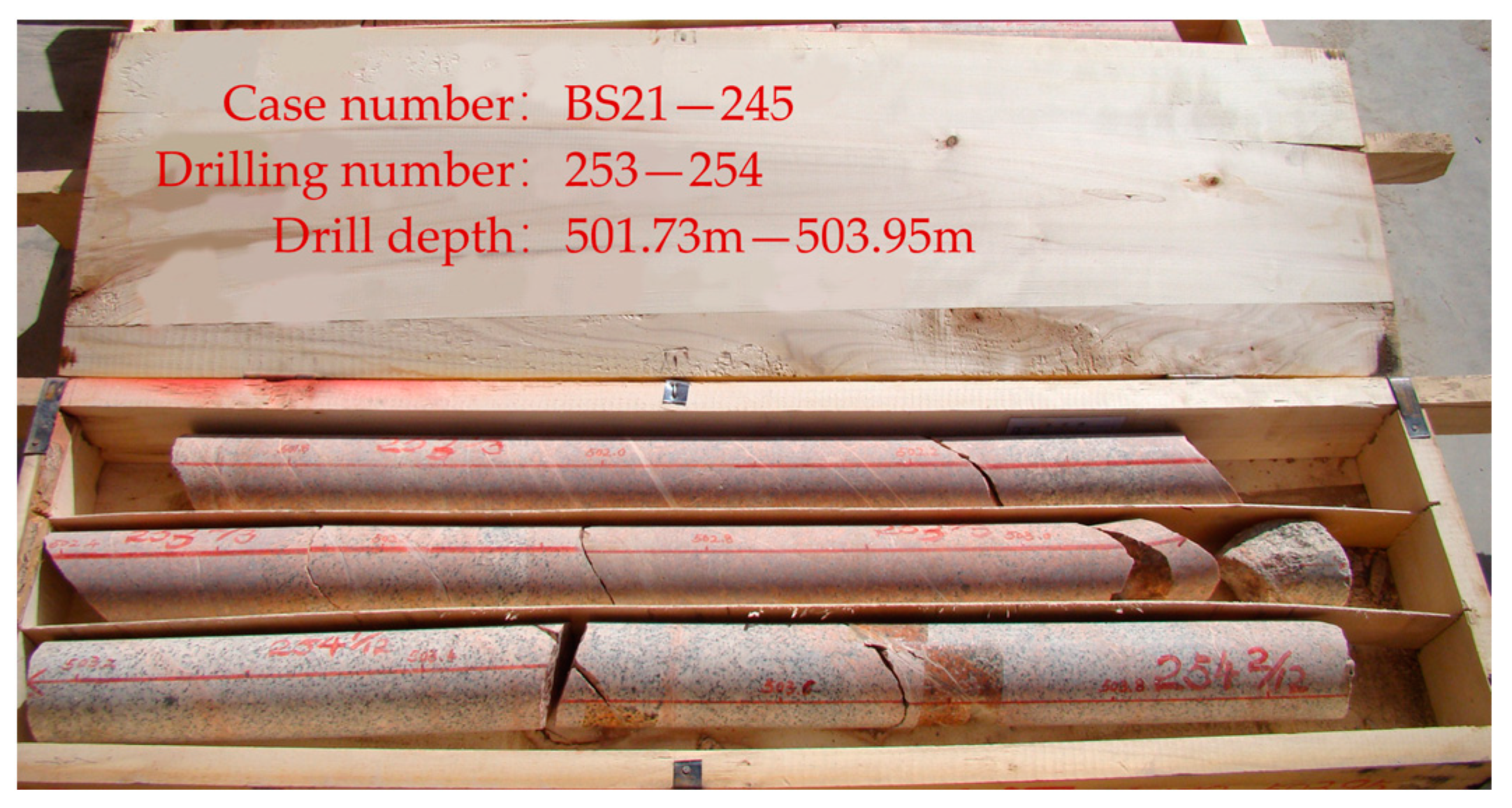
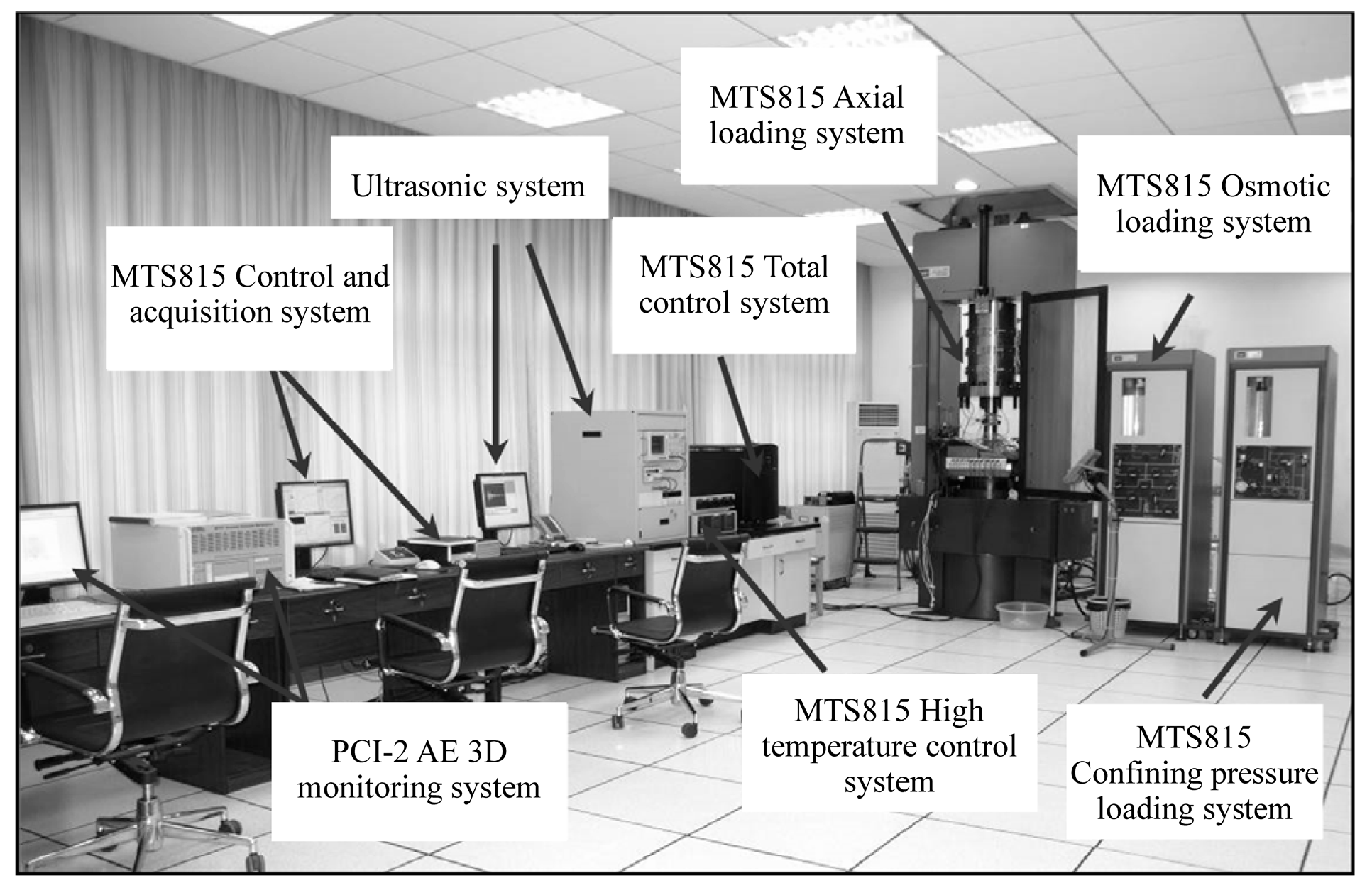
2.1. Experimental Equipment

The specimens were obtained from the pre-selected area of the Gansu Beishan site, which is a potential location for the high-level radioactive waste disposal facility in China. A geological drilling rig with a drill bit of 122 mm was used to drill the underground for core extraction; rock cores with a burial depth of about 500 mm was selected and transported to the laboratory for processing the standard specimens (Figure 1). The specimens were processed according to the precise requirements and dimensions of the experiment, resulting in standard specimens with a diameter of 50 mm and a height of 100 mm. The allowable deviation range of diameter is less than 0.2 mm, the allowable deviation range of unevenness on both ends is less than 0.05 mm, and the vertical deviation between two end faces and the axis does not exceed ±0.25°.

The experiments were conducted using the MTS815 Flex Test GT rock mechanics testing system, which is manufactured in the United States (Figure 2). The specimen is located in center of the test bed (Figure 3). In this experiment, the PCI-2 AE detection system produced by a physical acoustics company in the United States was used to detect the AE events. The acquisition frequency of AE sensors was set to 200 kHz, and the threshold value for signal acquisition was set to 26 dB. Amplification factor for signal acquisition was set to 40. The arrangement of the AE sensors is shown in Figure 3. Each specimen is symmetrically equipped with eight AE sensors, which are evenly arranged on the upper and lower sections. The center of the bottom surface of the specimen is the origin of the coordinates, with the y-axis being in the vertical direction and the x-axis and z-axis being in the horizontal direction. The coordinates of each sensor are shown in

Table 1. Detailed coordinates of AE sensors.

Numbers	1	2	3	4	5	6	7	8
x (mm)	0	180	0	−180	0	180	0	−180
y (mm)	140	140	140	140	0	0	0	0
z (mm)	180	0	−180	0	180	0	−180	0

. In the beginning of the experiment, the AE detection system and the loading equipment were started simultaneously to ensure that both devices recorded AE and mechanical data at the same time. During the experiment, extensometers were used to measure the axial and circumferential deformation of the specimens. Extensometers are produced by China Changchun Chuangyuan Testing Equipment Co., Ltd. (Changchun, China), and the testing accuracy of the is extensometers is 0.001 mm.

2.2. Experimental Methodology

The experiment adopts the combined axial load and circumferential deformation control loading process. During the experiment, axial load was first applied at a rate of 30 kN/min. When the evolumetric strain reached a turning point, the axial load control was stopped, and circumferential deformation control was used; the loading rate was set at 0.02 mm/min until the specimen failed. According to the stress characteristics of the Beishan and the depth of the underground laboratory, the confining pressures were set at 5 MPa, 10 MPa, and 30 MPa, denoted as specimen 1-1, 1-2, and 1-3, respectively.

3. Analysis of Test Results

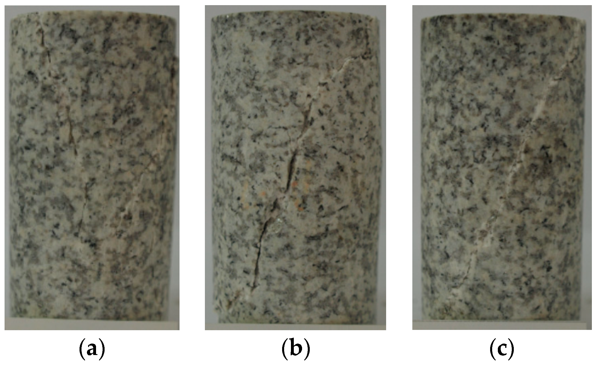
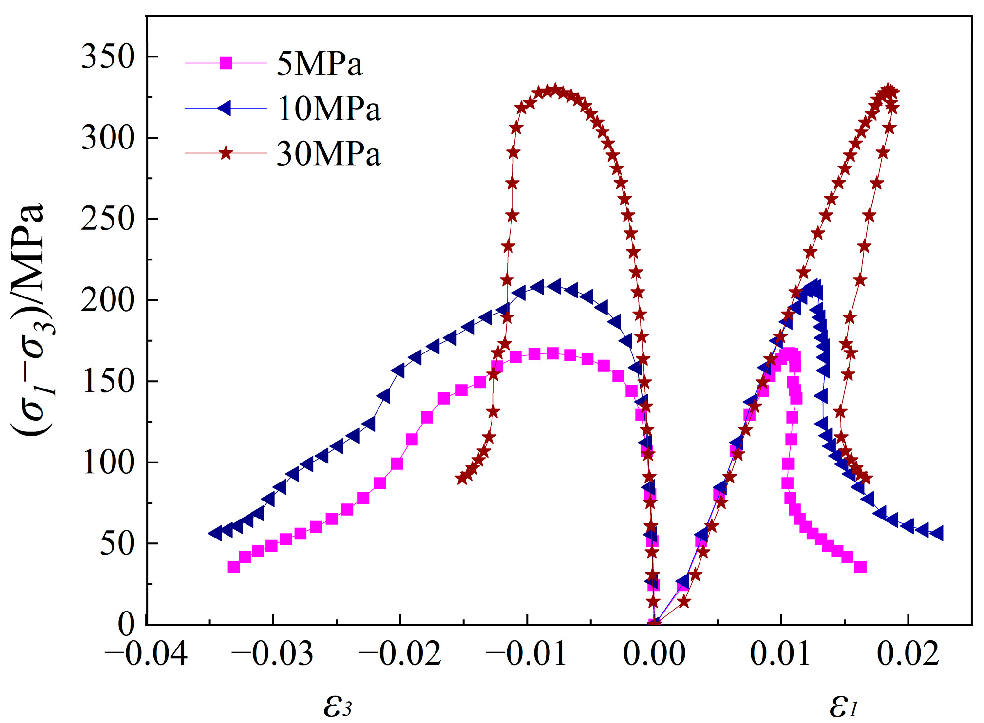
3.1. Basic Mechanical Properties

As the confining pressure increases, the peak strength of the rock significantly increases. With the confining pressure increasing from 5 MPa to 30 MPa, the peak strength increases from 166.62 MPa to 328.81 MPa (Figure 4 and Figure 5). There is no evident plastic characteristic after the peak of the specimen; as the confining pressure increases, the post-peak failure strain of the specimen decreases, and the energy release becomes more intense, leading to more severe failure. For instance, when the confining pressure reaches 30 MPa, significant rebound in axial deformation occurs after the peak and unstable failure occurs, exhibiting a type II stress–strain curve for rock failure.

Based on the characteristics of circumferential and axial deformation, the rock failure process can be divided into four stages: (1) closure stage of fracture, (2) linear elastic stage, (3) stable expansion stage of cracks, and (4) unstable expansion stage of cracks. The initiation, propagation, accumulation, and penetration of fractures mainly occur in the stable expansion stage and the unstable expansion stage of fractures. Therefore, the fracture failure characteristics are mainly determined by these two stages, corresponding to the characteristic stresses of initiation stress σ_ci, damage stress σ_cd, and peak stress σ_f. As shown in

Table 2. Characteristic stress of Beishan granite under different confining pressure.

σ3/MPa	σci/MPa	σcd/MPa	σf/MPa	σci/σf	σcd/σf	σci/σcd
1-1	67.16	117.91	166.62	0.403	0.707	0.569
1-2	80.11	159.78	208.13	0.385	0.768	0.501
1-3	122.59	267.60	328.81	0.373	0.814	0.458

, with the increase in confining pressure, the initiation stress, damage stress, and peak stress of the rock increase.

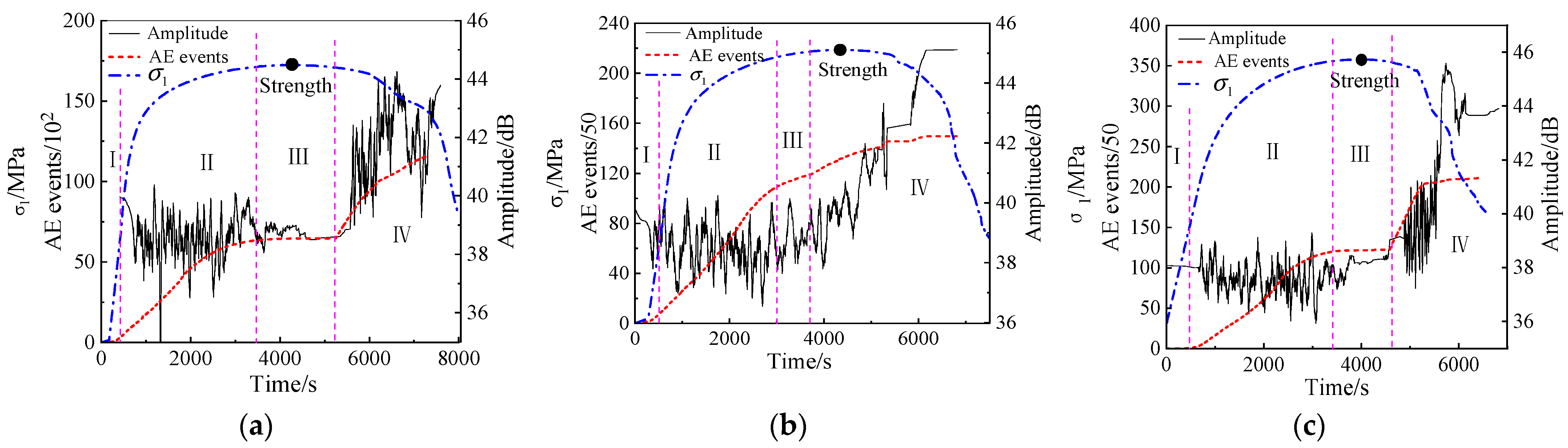
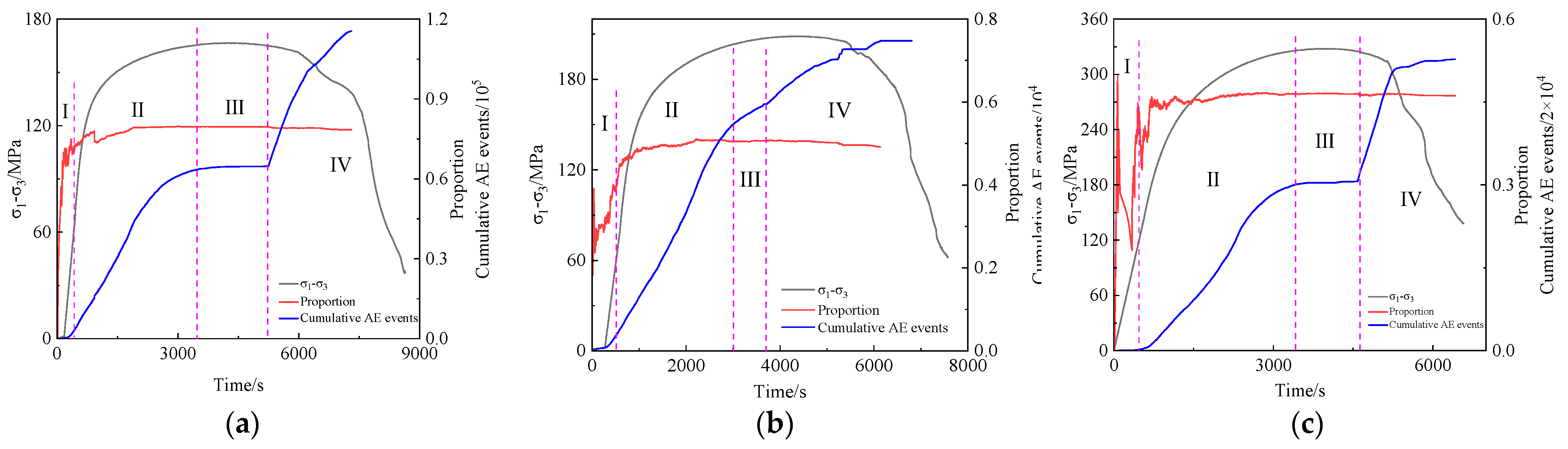
3.2. Characteristics of AE

According to the number of AE events, the damage process can be divided into four stages: the initial stage (I), the active stage (II), the calm stage (III), and the failure stage (IV) (as shown in Figure 6). The initial stage of AE is present during the closure stage of fracture and the linear elastic stage. In this stage, the AE events are sporadically distributed, and there are hardly any new cracks generated; the AE mainly originates from the compaction of the original cracks, and the amplitude fluctuations during this stage are not significant. The active stage of AE starts from approximately 40% of the peak stress and ends when the stress reaches 98% of the peak stress; in this stage, a large number of cracks are generated, extended, and connected, which is the main stage of crack initiation and propagation; the amplitude exhibits obvious fluctuations, but the change in the center of fluctuations is not significant. During the calm stage, the number of newly generated acoustic emissions decreases sharply, which is mainly due to the fact that a significant number of cracks have already formed within the rock mass, and the stress is redistributed at crack tips. In this stage, internal fractures undergo a process of large crack extension to the initiation and propagation of small cracks; the amplitude fluctuations during this stage decrease, and in some specimens, the fluctuations disappear. In the failure stage, stress concentration occurs on the fracture surface, and the cracks further extend until they become interconnected; also, the number of AE events rapidly increases, and the amplitude shows a significant increase with fluctuations.

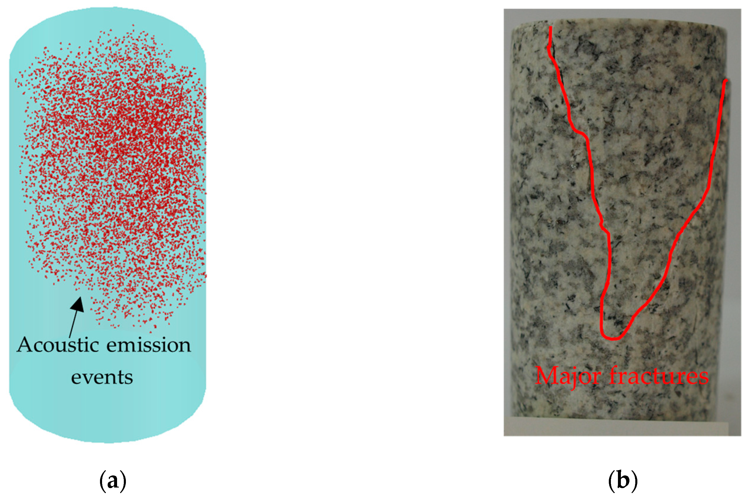
4. Evolutionary Characteristics of Major Fractures

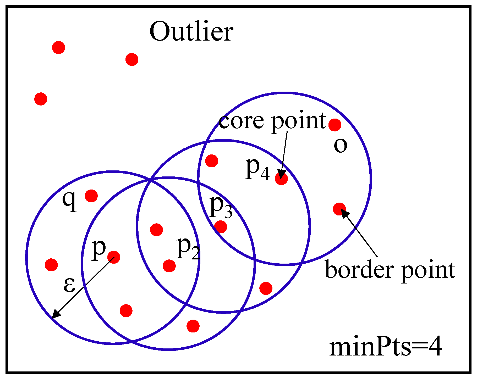
4.1. DBSACN Algorithm

DBSCAN (Density-Based Spatial Clustering of Applications with Noise) is a density-based clustering algorithm that has the advantages of not requiring the number of clusters, the ability of handling clusters of arbitrary shapes, and effectively discovering noise points. DBSCAN algorithm only requires the determination of two parameters, ε and minPts. ε refers to the radius of the neighborhood region around a point, and minPts refers to the minimum number of points required in the neighborhood region (Figure 7). Some basic concepts of DBSCAN are defined as follows:

(1)

ε-neighborhood: A region within a radius of ε around an object is called the ε-neighborhood of the object.

(2)

Core object: An object is considered as a core object if the number of sample points within its ε-neighborhood is greater than or equal to minPts.

(3)

Directly density-reachable: For a given set D, if point q is within the ε-neighborhood of p, and p is a core object, then q is directly density-reachable from p.

(4)

Density-reachable: For a given set D, if there is a sequence of sample points p₁, p₂, …, p_n, where p = p₁ and q = p_n, and if each object p_i is directly density-reachable from p_i-1, then q is density-reachable from p.

(5)

Density-connected: Points p and q are density-connected if p and q are directly density-reachable from o.

The goal of DBSCAN is to find the largest set of points that are density-connected. Based on ε and minPts, the points in the dataset can be classified into three categories:

(1)

Core point: These are points whose number of samples in the ε-neighborhood is greater than or equal to minPts.

(2)

Border point: These are points whose number of samples in the ε-neighborhood is less than minPts, but the points can be obtained from some core points (density-reachable, or directly density-reachable).

(3)

Outlier: Points that are neither core points nor boundary points are referred to as outliers or noise points.

4.2. Method for Determining DBSCAN Parameters

DBSCAN algorithm is a density-based clustering algorithm that does not require a pre-set number of clusters. However, it requires pre-determination of two parameters, ε and minPts, which describe the density of the data points. The clustering results are highly sensitive to the values of ε and minPts. Choosing inappropriate values may result in poor clustering performance or even clustering errors. One commonly used method to determine the values of ε is the k-nearest distance method, which involves the following steps:

(1)

The distances between objects in the set D are calculated to obtain the distance matrix Dist_n×n

$$Dis{t}_{n\times n}=\left\{dist(i,j),1\le i\le n,1\le j\le n\right\}$$

(1)

where n represents the number of data points in the uncategorized dataset D, Dist_n×n is a real symmetric matrix with n rows and n columns, dist(i, j) represents the distance from the i-th object to the j-th object in set D, and dist(i, j) is calculated using the Euclidean distance, expressed as Formula (2).

$$dist(i,j)=\sqrt{{\displaystyle \sum _{k=1}^m{(x_{ik}-x_{jk})}^2}}$$

(2)

where m represents the number of features for each element, x_ik denotes the value of the k-th feature parameter of the i-th element, and x_jk represents the numerical value of the k-th feature parameter of the j-th element.

(2)

Each row of the matrix Dist_n×n is sorted in an ascending order. Each row represents a ranking of the distances from the corresponding data point to all the other points. After sorting, Dist_n×k will be a collection of the k-th closest distance values to each data point.

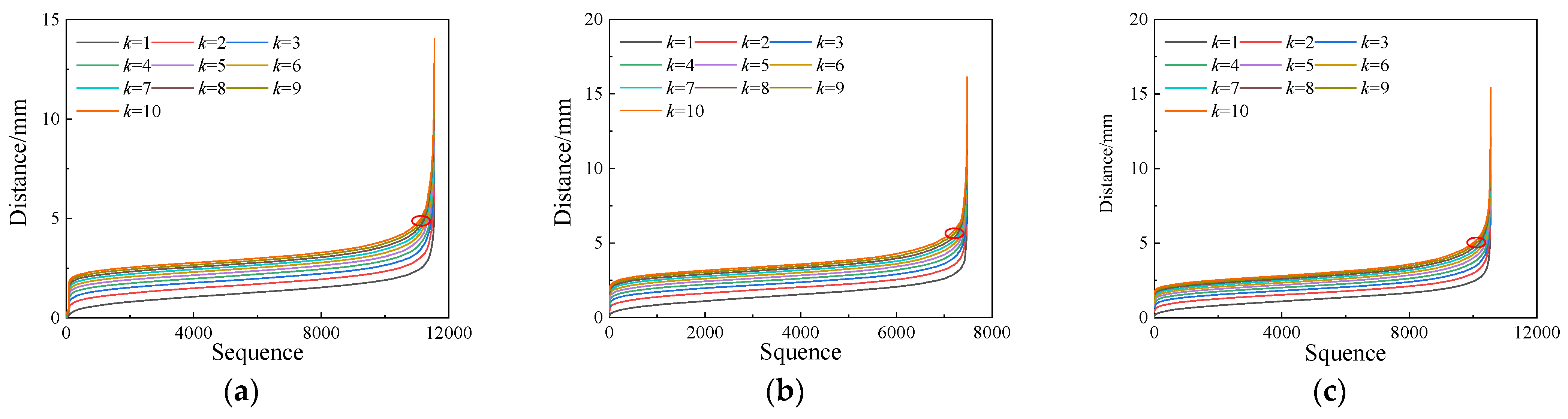
(3)

Column of the matrix Dist_n×n is sorted in an ascending order, and the curve graph of the k-th column (referred to as the k-curve) is plotted. The distance corresponding to the steep inflection point of the k-curve is the ε determined using the k-nearest neighbor distance method. By analyzing the change in the steep inflection points as k increases, it is observed that after a certain threshold, steep inflection points of k-curve concentrate in a specific region; this indicates that with the increase in k, outlier points remains essentially the same, and both the clustering point and outlier point detection results tend to stabilize (Ester et al. [22]). The distance value corresponding to the region of concentration of steep inflection points in the k-curve is taken as the ε value.

(4)

The expectation method is used to generate MinPts. For ε, the number of objects within the ε-neighborhood of each data point is calculated sequentially. The mathematical expectation of the number within ε-neighborhoods for all data points is then computed, and this value is taken as the MinPts for set D.

$$MinPts=\frac{1}{n}{\displaystyle \sum _{i=1}^n{P}_i}$$

(3)

where P_i represents the number of objects within the ε-neighborhood of the i-th data point, and n represents the total number of data points.

4.3. DBSCAN Parameters and Major Fractures

Spatial location information of each AE is used as data features, so each data point contains three coordinates: x, y, and z. Based on the location information of AE events, distances between each AE event was calculated, and k-curves for different specimens were plotted (Figure 8). The shapes of k-curves for different specimens are generally similar: in the initial and middle stages, k-curves are relatively flat, but in the end stage, they are steep. Through observing the k-curves of different specimens, it can be noticed that when k is less than 5, the steep inflection points vary significantly; however, when k is greater than 5, the steep inflection points tend to concentrate within a smaller region (highlighted by a red circle in Figure 8). The corresponding distance values in the concentrated region are taken as the ε.

MinPts values for each specimen was calculated based on the ε values and Formula (3) (

Table 3. DBSCAN parameters and clustering results.

Number	ε	minPts	Number of Categories	Main Fractures	Non-Main Fractures	Outlier Fracture	Proportion of Main Failures %	Proportion of Non-Main Fractures %	Proportion of Outlier Fracture %
1-1	5	45.39	4	9067	154	2330	79.56	1.33	20.17
1-2	5.5	34.49	2	3675	48	3756	49.40	0.64	50.22
1-3	5	45.91	1	4868	0	5683	46.14	0.00	53.86

); then, the classification of different AE specimens was determined through the DBSCAN algorithm. The largest cluster is referred to as the major fracture, and outliers are referred to as outlier fractures. Clusters that are not the major fracture or outlier fractures are classified as non-major fractures. Non-major fractures and outlier fractures are collectively referred to as other fractures. Space distribution of major fracture is basically similar to the major fracture image of failure specimen (Figure 9). As the confining pressure increases, fracture categories reduce, the proportions of major and non-major fractures decrease, and the proportion of outlier fractures increases. This is mainly because, when the confining pressure is low, the original defects have a greater influence on the development of internal cracks, making it easy for the cracks to cluster around the original defects. However, as the confining pressure increases, the influence of the original defects on the development of crack is weakened; additionally, as the confining pressure increases, the distribution of internal rock crack becomes more uniform, leading to less clustering of fractures.

4.4. Characteristics of the Variation in the Quantity of Main Fractures

The cumulative number of AE events, the proportion of major fractures, and the variation in stress over time are shown in Figure 10. In the initial stage, AE events are randomly distributed in space and exhibit a disordered state; therefore, the proportion of major fractures significantly fluctuates, showing weak regularity. In the active stage of AE, a large number of cracks are generated, expanded, and interconnected. In this stage, the internal fractures gradually transfer from a disordered state to an ordered state, and as a result, the proportion of main fractures in AE events shows an increasing trend, and the increase is relatively drastic. During the calm stage, the number of AE events sharply decreases, while the proportion of main fractures remains relatively constant. In the failure stage, stress concentration occurs on the fracture plane, and the cracks further expand and connect; the number of AE events rapidly increases at this stage due to the presence of numerous fractures inside the specimen and stress redistribution, and there is an increase in AE events produced by other fractures, leading to a slight decrease in the proportion of major fractures.

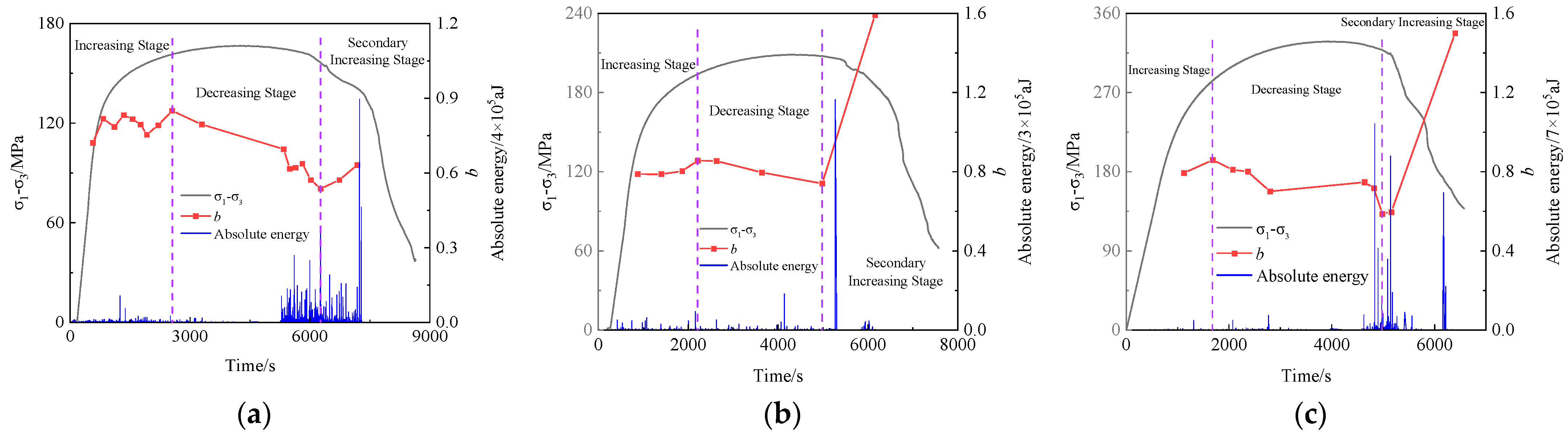
4.5. b-Values of Acoustic Emissions for Major Fracture

Once an AE event is treated as a slight vibration, the characteristics of rock deformation and failure processes can be analyzed through the related parameters of magnitude and frequency, represented by the b-value. The b-value of acoustic emissions is calculated using the G-R relationship proposed by Gutenberg B. and Richter C. F. [23]. The G-R relationship formula for acoustic emissions is as follows:

$$\lg N=a-b\lg Q$$

(4)

where Q represents the absolute energy which is derived from the integral of the squared voltage signal divided by the reference resistance (10k-ohm) over the duration of the AE waveform packet, N is the number of events with energy greater than or equal to Q, a and b are constants. In a statistical sense, the b-value represents the proportion of small AE events. An increase in the b-value indicates an increase in the proportion of small AE events, which suggests an increase in the expansion of small fractures and an increase in the relative stability of the rock. On the other hand, a decrease in the b-value indicates a decrease in the proportion of small fractures, which indicates an increase in the number of rapidly expanding large fractures and a decrease in rock stability. In this article, b-value is calculated for every 500 AE events.

The variation in the b-value with time is shown in Figure 11, and the relationship between b-value, time, and stress is shown in

Table 4. Relationship between b and time.

Specimens	b Value	Time/s	Stress/MPa
1-1	increasing stage	0–2553.12	0–161.49
	decreasing stage	2553.12–6268.07	161.49–156.33
	secondary increasing stage	6268.07–end	156.33–end
1-2	increasing stage	0–2211.79	0–193.88
	decreasing stage	2211.79–4981.08	193.88–207.72
	secondary increasing stage	4981.08–end	207.72–end
1-3	increasing stage	0–1678.52	0–282.86
	decreasing stage	1678.52–4981.78	282.86–318.31
	secondary increasing stage	4981.78–end	318.31–end

. The overall change in the b-value can be divided into three stages: increasing stage, decreasing stage, and secondary increasing stage. During the increasing stage, b-value shows an overall upward trend, indicating a dominance of small energy AE events and relative stability of the specimen. The decreasing stage is mainly concentrated around the peak point, with b-value showing an overall downward trend, which suggests an increasing proportion of high energy AE events, indicating stability deterioration of the specimen and occurrence of failure. The secondary increasing stage is characterized by an increase in the b-value, indicating a higher proportion of low energy AE events and enhanced stability of the specimen; this is primarily attributed to the redistribution of internal stresses after specimen failure, leading to a new equilibrium state. Mogi [24] discovered the same pattern while studying the variation in the b-value during the process of strong earthquakes; so the evolution law of the b-value in rock failure is the same as that in strong earthquakes formation process, which indicate the self-similarity of the seismic process, both for earthquakes of biggest energies (magnitudes) and for microcracks in rocks.

5. Identification and Prediction of Major Fractures

5.1. Methods for Major Fractures Identification

Neural networks are parallel interconnected networks composed of simple units, which can simulate the interactive responses of biological systems to real-world objects (Kohonen [25]). The basic component in a neural network is a neuron model (Figure 12). A basic neuron consists of input values, output values, and an activation function. Operational process of a basic neuron is as shown in Formula (5).

$$y=f\left({\displaystyle \sum _{i=1}^n{\omega }_i{x}_i-\theta }\right)$$

(5)

where i represents the number of input features, x_i represents the i-th feature of neuron input, ω_i represents the connection weight of the i-th feature, θ represents the threshold, f represents the activation function, and y represents the output value. A neural network is composed of a large number of neurons and includes one input layer, one output layer, and several hidden layers. Different values of ω_i and θ will lead to different outputs, resulting in errors between the output of the neural network and the real data. The error is calculated using Formula (6). A neural network is trained to minimize the mean squared error (MSE). The calculation formula for the mean squared error is expressed as Formula (7).

$$E_k=\frac{1}{2}{\displaystyle \sum _{j=1}^l{({\widehat{y}}_j^k-y_j^k)}^2}$$

(6)

$$E=\frac{1}{m}{\displaystyle \sum _{k=1}^m{E}_k}$$

(7)

where k represents the total number of training samples, j represents the number of units in the output layer, $y_j^k$ represents the true value corresponding to the k-th data in the sample, ${\widehat{y}}_j^k$ represents the output value corresponding to the k-th data in the sample, E_k represents the error of the k-th data, and E represents the mean squared error of the training samples.

The error of the BP artificial neural network is minimized through backpropagation. The BP artificial neural network has the advantages of strong self-learning, self-organization, adaptivity, and fault tolerance. It also has fast computation speed, and has been widely used in various fields such as tunnel excavation, disaster prediction, and energy extraction. Therefore, this paper adopts the BP neural network for identifying the main rupture.

5.2. Results of the Main Rupture Prediction

In order to reduce the influence of different fractures sample quantities on the identification results, 2300 AE data were randomly selected from both the major fractures and other fractures, respectively. Among those AE events, 4000 AE data were used as the training data, and 600 AE data were used as the test data. Each datum contains 21 feature information of acoustic emissions, including amplitude, frequency, energy, rise time, and so on. The constructed neural network consists of one input layer, one output layer, and four hidden layers, with each hidden layer containing sixteen units. The activation function is the logarithmic sigmoid transfer function; the training method used is gradient descent, and the number of training epochs is set to 6000.

The recognition model established through the BP neural network is used to recognize both the training and testing data. As shown in

Table 5. Identification results of fracture mode through the BP neural network.

Specimen	Accuracy for Traindata/%			Accuracy for Testdata/%
	Whole	Main Fracture	Other Fracture	Whole	Main Fracture	Other Fracture
1-1	96.33	95.70	96.96	95.18	93.33	97.00
1-2	81.25	78.75	83.75	76.67	83.68	69.67
1-3	78.83	88.30	69.35	76.67	84.67	68.67
Average Value	85.47	87.58	83.35	82.83	87.22	78.44

, the model has an average accuracy of 85.47% for the training data, and an average accuracy of 82.83% for the testing data. The overall average accuracy of the model for both the training and testing data is above 80%, indicating that the established model is effective in recognizing various forms of fractures. The highest accuracy for identifying the main fracture in the testing data is for specimen 1-1, with 93.33%, and the lowest accuracy is for specimen 1-2, with 83.68%. The average accuracy for identifying the main fracture in the testing data is 87.22%, while the average accuracy for identifying other fractures in the testing data is 78.44%. The accuracy for identifying the main fracture is significantly higher than the accuracy for identifying other fractures.

6. Conclusions

A triaxial AE experiment was carried out on the Beishan high-level radioactive waste disposal repository, and methods such as fractal theory and machine learning were utilized to analyze the AE characteristics during rock failure. The evolution of fracture clusters within the rock was studied, and the AE characteristics of different fracture clusters were analyzed. The conclusions are as follows:

(1)

As the confining pressure increases, categories of fracture reduce, the proportion of major and non-major fractures decrease, and the proportion of outlier fractures increases;

(2)

During the initial phase, the proportion of major fractures AE significantly fluctuates, while during the active phase, proportion of major fracture AE generally increases. The proportion of major fracture AE remains relatively constant during the calm phase, and slightly decreases in the destructive phase;

(3)

The variation in the b-value of major fractures during the process of rock failure can be divided into three stages—increase, decrease, and secondary increase—which indicates that microcracks in rocks also has the self-similarity aspect of the seismic process;

(4)

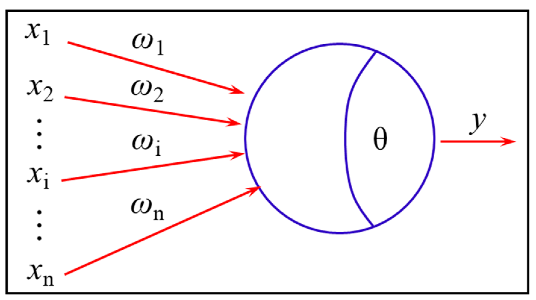
A rock major fracture identification model was established based on a BP neural network, and the model’s accuracy rate of major fracture identification was 87.22%.

References

1. Das, R.; Singh, T.N. A novel technique for temporal evolution of rockburst in underground rock tunnel: An experimental study. Environ. Earth Sci. 2022, 81, 420. [Google Scholar] [CrossRef]
2. Jin, H.; Gao, B.; Shen, Y. Model analysis of sandstone tunnel cracking based on fracture mechanics theory and sensor testing technology research. J. Sens. 2022, 2022, 2482638. [Google Scholar] [CrossRef]
3. Zhang, L.; Chao, W.; Liu, Z.; Cong, Y.; Wang, Z. Crack propagation characteristics during progressive failure of circular tunnels and the early warning thereof based on multi-sensor data fusion. Geomech. Geophys. Geo-Energy Geo-Resour. 2022, 8, 172. [Google Scholar] [CrossRef]
4. Manuello, A.; Niccolini, G.; Carpinteri, A. AE monitoring of a concrete arch road tunnel: Damage evolution and localization. Eng. Fract. Mech. 2019, 210, 279–287. [Google Scholar] [CrossRef]
5. Huang, Y.; Yang, S.; Ranjith, P.G.; Zhao, J. Strength failure behavior and crack evolution mechanism of granite containing pre-existing non-coplanar holes: Experimental study and particle flow modeling. Comput. Geotech. 2017, 88, 182–198. [Google Scholar] [CrossRef]
6. Belikov, V.T.; Kozlova, I.A.; Ryvkin, D.G.; Yurkov, A.K. The character of evolution of rock fracture processes from observations of acoustic emission and time variations in radon volumetric activity. Izv. Phys. Solid Earth 2020, 56, 425–436. [Google Scholar] [CrossRef]
7. Damaskinskaya, E.E.; Hilarov, V.L.; Panteleev, I.A.; Gafurova, D.R.; Frolov, D.I. Statistical regularities of formation of a main crack in a structurally inhomogeneous material under various deformation conditions. Phys. Solid State 2018, 60, 1821–1826. [Google Scholar] [CrossRef]
8. Panteleev, I.A. Analysis of the seismic moment tensor of acoustic emission: Granite fracture micromechanisms during three-point bending. Acoust. Phys. 2020, 66, 653–665. [Google Scholar] [CrossRef]
9. Hou, X.; Zhai, H.; Wang, C.; Wang, T.; He, X.; Sun, X.; Bai, Z.; Zhou, B.; Li, X. Spatial Characterization of Single-Cracked Space Based on Microcrack Distribution in Sandstone Failure. Appl. Sci. 2023, 13, 1462. [Google Scholar] [CrossRef]
10. Damaskinskaya, E.E.; Panteleev, I.A.; Kadomtsev, A.G.; Naimark, O.B. Effect of the state of internal boundaries on granite fracture nature under quasi-static compression. Phys. Solid State 2017, 59, 944–954. [Google Scholar] [CrossRef]
11. Wang, T.; Wang, L.; Xue, F.; Xue, M. Identification of crack development in granite under triaxial compression based on the acoustic emission signal. Int. J. Distrib. Sens. Netw. 2021, 17, 1550147720986116. [Google Scholar] [CrossRef]
12. Nakayama, S.; Watanabe, Y.; Kato, M. Regulatory research for geological disposal of high-level radioactive waste in Japan. In Proceedings of the 13th International Conference on Environmental Remediation and Radioactive Waste Management, Tsukuba, Japan, 3–7 October 2010. [Google Scholar]
13. Kitamura, A.; Doi, R.; Yoshida, Y. Evaluated and estimated solubility of some elements for performance assessment of geological disposal of high-level radioactive waste using updated version of thermodynamic database. In Proceedings of the 13th International Conference on Environmental Remediation and Radioactive Waste Management, Tsukuba, Japan, 3–7 October 2010. [Google Scholar]
14. Ren, M.; Zhang, Q.; Liu, C.; Wu, D.; Ding, Y. The elastic–plastic damage analysis of underground research laboratory excavation for disposal of high level radioactive waste. Geotech. Geol. Eng. 2019, 37, 1793–1811. [Google Scholar] [CrossRef]
15. Wang, J.; Su, R.; Chen, W.; Guo, Y.; Jin, Y.; Wen, Z.; Liu, Y. Deep geological disposal of high-level radioactive wastes in China. Chin. J. Rock Mech. Eng. 2006, 25, 649–658. [Google Scholar]
16. Rao, Z.; Li, G.; Liu, X.; Liu, P.; Li, H.; Liu, S.; Zhu, M.; Guo, C.; Ni, F.; Gong, Z.; et al. Fault activity in clay rock site candidate of high level radioactive waste repository, Tamusu, Inner Mongolia. Minerals 2021, 11, 941. [Google Scholar] [CrossRef]
17. Wu, Y.; Li, X.; Huang, Z.; Xue, S. Effect of temperature on physical, mechanical and acoustic emission properties of Beishan granite, Gansu Province, China. Nat. Hazards 2021, 107, 1577–1592. [Google Scholar] [CrossRef]
18. Zhou, H.; Wang, Z.; Wang, C.; Liu, J. On acoustic emission and post-peak energy evolution in Beishan granite under cyclic loading. Rock Mech. Rock Eng. 2019, 52, 283–288. [Google Scholar] [CrossRef]
19. Miao, S.; Pan, P.; Zhao, X.; Shao, C.; Yu, P. Experimental study on damage and fracture characteristics of Beishan granite subjected to high-temperature treatment with DIC and AE techniques. Rock Mech. Rock Eng. 2021, 54, 721–743. [Google Scholar] [CrossRef]
20. Zhao, X.; Wang, J.; Cai, M.; Cheng, C.; Ma, L.; Su, R.; Zhao, F.; Li, D. Influence of unloading rate on the strainburst characteristics of Beishan granite under true-triaxial unloading conditions. Rock Mech. Rock Eng. 2014, 47, 467–483. [Google Scholar] [CrossRef]
21. Wang, C.; Liu, J.; Zhao, Y.; Han, S. Mechanical properties and fracture evolution process of Beishan granite under tensile state. Bull. Eng. Geol. Environ. 2022, 81, 274. [Google Scholar] [CrossRef]
22. Ester, M.; Kriegel, H.-P.; Sander, J.; Xu, X. A density-based algorithm for discovering clusters in large spatial databases with noise. In Proceedings of the Knowledge Discovery and Data Mining; AAAI Press: Portland, OR, USA, 1996; pp. 226–231. [Google Scholar]
23. Gutenberg, B.; Richter, C.F. Frequency of earthquakes in California. Bull. Seismol. Soc. Am. 1944, 34, 185–188. [Google Scholar] [CrossRef]
24. Mogi, K. Two kinds of seismic gaps. Pure Appl. Geophys. 1979, 117, 1172–1186. [Google Scholar] [CrossRef]
25. Kohonen, T. An introduction to neural computing. Neural Netw. 1988, 1, 3–16. [Google Scholar] [CrossRef]
Figure 1. Image of drill core.
Applsci 13 10355 g001
Figure 2. MTS815 Flex Test GT Rock mechanics test system.
Applsci 13 10355 g002
Figure 3. Layout of AE sensors.
Applsci 13 10355 g003
Figure 4. Stress–strain curves of granite under different confining pressures.
Applsci 13 10355 g004
Figure 5. Images of failure specimens: (a) 1-1; (b) 1-2; (c) 1-3.
Applsci 13 10355 g005
Figure 6. Curves of AE hits, AE amplitude and stress with time: (a) 1-1; (b) 1-2; (c) 1-3.
Applsci 13 10355 g006
Figure 7. Illustration of the basic concept of DBSCAN.
Applsci 13 10355 g007
Figure 8. k-curves of different specimens: (a) 1-1; (b) 1-2; (c) 1-3.
Applsci 13 10355 g008
Figure 9. Major fractures of 1-2: (a) space distribution of major fracture determined via DBSCAN; (b) major fracture of image.
Applsci 13 10355 g009
Figure 10. Curves of AE events, proportion and stress with time: (a) 1-1; (b) 1-2; (c) 1-3. Where, I represents the initial stage, II represents the active stage of AE, III represents the calm stage, and IV represents the failure stage.
Applsci 13 10355 g010
Figure 11. Curves of b-value, absolute energy and stress with time: (a) 1-1; (b) 1-2; (c) 1-3.
Applsci 13 10355 g011
Figure 12. Model of neuron.
Applsci 13 10355 g012