Bayesian Network Demand-Forecasting Model Based on Modified Particle Swarm Optimization

Abstract

With the increasing variety of products, the increasing substitutability of products, and the trend of customized products, the volatility of market demand is increasing, which poses a challenge to make accurate demand forecasting. The Bayesian method is particularly promising and appealing when the data fluctuate greatly. This paper proposes a product-demand forecasting model based on multilayer Bayesian network, which introduces hidden layer variables and volatility factors to meet the time series connection and volatility of the demand data. However, most studies use sampling methods to estimate the parameters. We use Bayesian maximum a posteriori estimation to estimate the model parameters and introduce an improved particle swarm optimization algorithm (MPSO) to optimize the objective function. In order to increase the diversity of the particle population and accelerate the convergence, an adaptive particle velocity, position updating strategy, and nonlinear changing inertia weight are introduced in the algorithm. Finally, RMSE (Root Mean Square Error) and MAPE (Mean Absolute Percentage Error) are used as the evaluation criterion to conduct experiments on six different datasets, and the experimental results are compared with the results of the ARIMA (autoregressive integrated moving average model) method and PSO algorithm. The experimental results show that the method has a good prediction effect. It provides a new idea for demand forecasting in the supply chain.

1. Introduction

The current sales model has become diversified, and people are keen on online shopping. Nowadays, in addition to online retail platforms such as Taobao and Jingdong, more and more manufacturing companies have also opened online and offline sales channels, and customers’ shopping channels have become diversified. International market research company Euromonitor International shows that personality and customized products are important keywords for future consumption development in the world’s top ten consumption trends, and the demand for customized products is gradually increasing [1]. At the same time, the substitutability of products is increasing, and the volatility and uncertainty from market demand are increasing. In addition, in order to encourage consumers to consume, enterprises have adopted many artificial periodic promotional activities, which further increases the uncertainty of market demand. Under these influences, customer demand has gradually shown a higher degree of intermittence and explosiveness: more zeros and high-count islands [2].

1.1. Review of Demand Forecasting

Demand is the source of production and supply. Many scholars have shown that demand forecasting plays a key role in a company’s operational decision-making [3,4,5,6,7], and a large number of scholars have studied how to make accurate demand forecasting. From the perspective of modeling, some scholars have established parametric models and obtained the fixed parameters of the model by training and fitting the historical data so as to predict the future demand. Some scholars established a nonparametric model, regarded the model parameters as random variables, obtained different parameters at different times through the training of historical data, and then predicted the future demand.

Most of the existing studies based on parametric models were constructed from the perspective of time series prediction. The commonly used methods include the ARIMA method [8,9,10,11,12,13,14,15] and exponential smoothing method [16,17,18,19]. In order to solve the nonlinear problems that may exist in the time series model, many scholars have improved the ARIMA method under different problem backgrounds, such as the nonlinear ARIMA time series model considering seasonal factors [10,11,12,13] and the combination forecasting method combined with computational intelligence methods [14,15]. Based on the network graph theory combined with the four attributes of the product, Haytham et al. proposed an autoregressive integrated moving average model (ARIMAX) with exogenous variables to predict the sales of cosmetics. The prediction results were compared with the Croston method and the ARIMA method, and better results were obtained [20].

These methods have achieved good prediction results. However, at present, there are many kinds of products, some of which show a low level of demand, as well as many periodic promotional activities, and the demand shows intervals and strong volatility. Johnston and Boylan cited an example where the average number of purchases of an item by a customer was 1.32 occasions per year, and ‘‘For the slower movers, the average number of purchases was only 1.06 per item [per] customer’’ [21]. For interval demand forecasting, the most classic method is the Croston method, which calculates the expected demand for the next period, that is, the ratio of the expected non-zero demand to the expected non-zero-demand time interval, both of which are estimated by simple exponential smoothing [22]. In general, if the parameter model is specified incorrectly, that is, the data seriously violates its basic model assumptions, it may lead to inconsistent predictions and ultimately lead to inappropriate inferences and suboptimal recommendations. A misspecified Bayesian model can yield an ill-behaved asymptotic posterior distribution [23,24,25]. The work in [26] finds that the outperformance of nonparametric methods increases with higher demand variability.

The nonparametric model has the ability to accommodate infinite attributes and infinite levels in theory, which can meet the needs of complex system characterization. Snyder et al. proposed the state space model and distribution prediction. The model tracks the expected demand by exponential-smoothing updates, assumes that the demand follows a negative binomial distribution, and uses the maximum-likelihood method to estimate the model parameters [27]. On the basis of Snyder, Chapados proposed Bayesian inference model H-NBSS for count-type time series. In order to adapt to the characteristics of counting data, H-NBSS uses the counting process as the statistical prior of the data, which makes the solution of the model very difficult. In addition, due to the characteristics of the counting process itself, H-NBSS is also extremely sensitive to the results of parameter adjustment, and subtle changes in model parameters may also lead to great fluctuations in prediction results [28]. Assuming that the demand distribution is a multistage Poisson distribution, Seeger et al. constructed a nonparametric Bayesian model [2]. Babai et al. proposed a nonparametric Bayesian method (CPB), assuming that the demand follows a compound Poisson-geometric distribution [26]. However, there is no known conjugate prior that leads to a posterior distribution in a closed form. Considering the volatility of function time series, Guillaume et al. proposed a local autoregressive nonparametric prediction model. The relevant parameters learn the inference through a strategy based on approximate Bayesian computation [29]. Yuan Ye et al. proposed a nonparametric Bayesian forecasting method based on the empirical Bayesian paradigm, which is very flexible in dealing with a variety of demand patterns and used the demand data of 46,272 inventory units of an auto parts distributor to evaluate the relative performance of the method [30]. Aiming at the problem of port volume prediction, Majid et al. proposed a prediction model based on Bayesian estimation. Mutual information analysis is added to the model, and the macroeconomic variables are regarded as random variables. The related uncertainty is quantified by the posterior distribution. 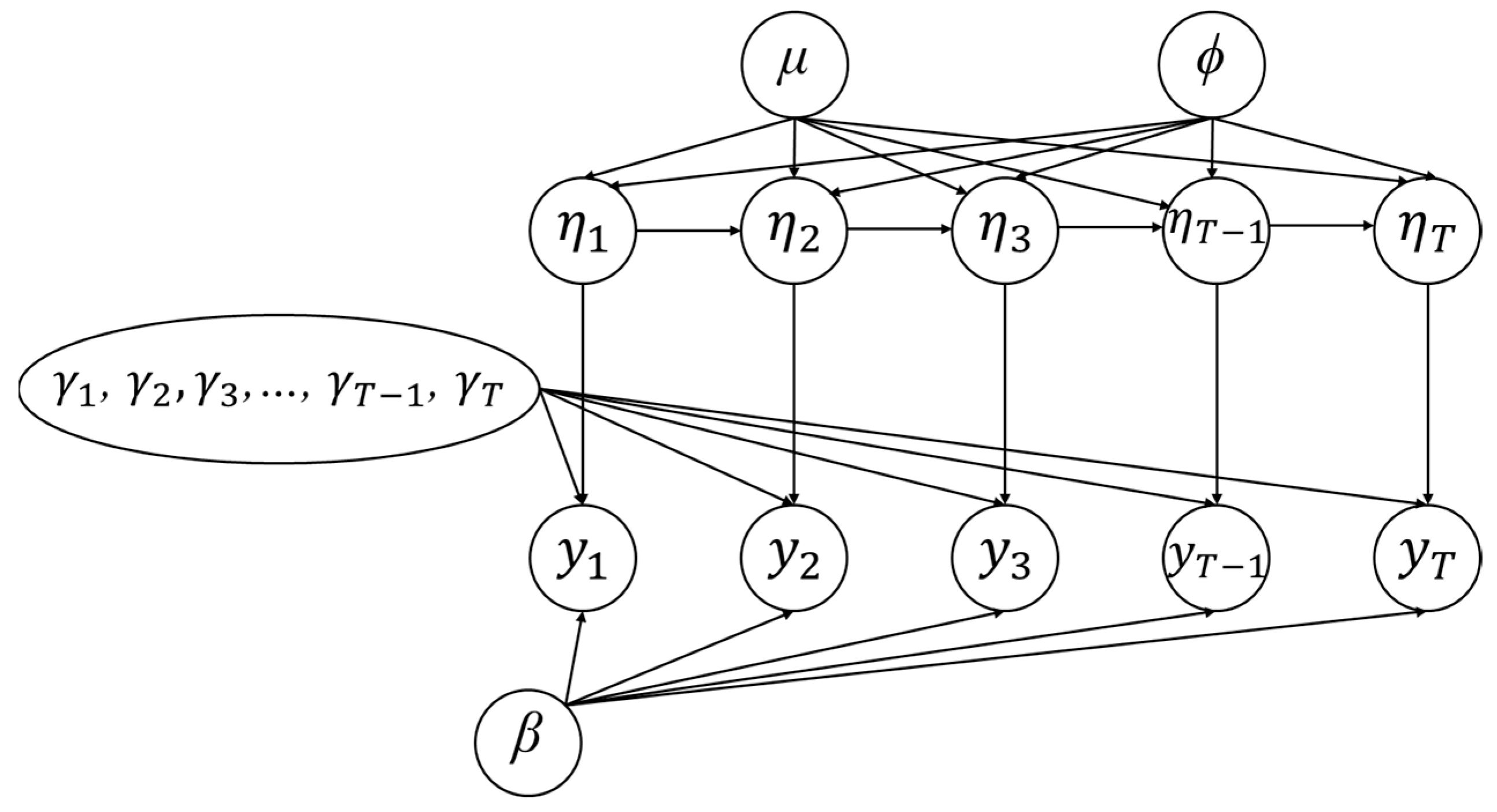However, this prediction method requires effective quantification of macroeconomic variables [31]. Kowsari et al. pointed out that the Bayesian method regards the regression coefficient as a random variable and considers the uncertainty of the parameters with the data as the condition. In the model hypothesis of this paper, the regression coefficient ϕ in the hidden layer variable η_t is assumed to obey the normal distribution, and the appropriate value is obtained through data training [32].

The Bayesian network is a probabilistic graphical model that combines the knowledge of probability theory and graph theory. It can reflect the potential dependencies between variables, deal with some uncertain causality, and effectively represent and calculate the joint probability distribution of a set of random variables. This structure has attracted much attention in statistics and artificial intelligence [33,34]. The Bayesian network is widely used in the energy, biology, medical, and other fields, such as wind-energy forecasting, power demand forecasting, and water resources demand forecasting. In many studies, the Bayesian network model is used for supply-chain demand forecasting.

The Bayesian network is based on Bayesian theory in practical application. It is worth pointing out that the Bayesian method shows the characteristics of experience and demand data in a quantifiable form by selecting an appropriate prior distribution. The variance in the prior distribution reflects the uncertainty of the demand data. As the demand evolves, the observed data are used to update the likelihood function to obtain the posterior distribution of the demand. The purpose of Bayesian posterior estimation is to find the appropriate parameter value. The prediction model in Section 2 mainly adopts the Bayesian method, which uses the Bayesian theorem to update the prior distribution (the probability specified before data collection) to the posterior distribution (the data after data analysis). In the parameter estimation process, we use the Bayesian maximum posterior estimation method to derive the functional form of the maximum posterior estimation.

Bayesian methods have been successful in many fields and predictive environments and are particularly promising and appealing when there are considerable changes in the data. This paper considers the construction of a multilayer Bayesian network commodity demand-forecasting model under the given historical sales data of commodities. The model considers the time series correlation of historical data as well as the volatility of demand and has strong flexibility. The maximum posteriori estimation method is used to estimate the optimal parameters, and then the commodity demand in the future is predicted according to the optimal parameters.

1.2. Review of PSO Algorithm

The particle swarm optimization (PSO) algorithm is an evolutionary computing technology based on swarm intelligence theory proposed by American psychologist Kennedy and electrical engineer Eberhart, inspired by the foraging behaviors of birds and fish [35]. Because of its simple concept, few parameters, fast convergence, and easy implementation, it is widely used in function optimization, production scheduling, pattern recognition, parameter estimation, and other fields. Let M particles form a group in a D-dimensional search space, and each particle is regarded as a search individual. They search for the individual that makes the objective function optimal in the search space. By changing their position and velocity vectors, they follow the individuals with higher fitness for optimization. In the t-th iteration, the position vector of each particle can be expressed as X_i(t) = (x_i1, x_i2, …, x_iD)^T, and the velocity vector can be expressed as V_i(t) = (v_i1, v_i2, …, v_iD)^T.

The equations for PSO can be expressed as follows:

$$\{\begin{array}{c}{v}_{id}(t+1)=w{v}_{id}(t)+c_{1}ran{d}_1(pbes{t}_{id}-x_{id}(t))+c_{2}ran{d}_2(gbes{t}_d-x_{id}(t))\\ x_{id}(t+1)=x_{id}(t)+v_{id}(t+1)\end{array}$$

(1)

where w is the inertia weight; c₁ and c₂ are acceleration coefficients; rand₁ and rand₂ are two uniformly distributed random numbers generated within [0,1]; pbest is the personal best point for the i-th particle; and gbest is the global best point.

The PSO algorithm has been widely popular because of its advantages of fewer computational memory requirements and fewer control parameters. However, it is easy to fall into the local minimum solution when solving complex nonlinear multimodal functions. In order to solve this problem, many scholars have made improvements in the inertial weight w and particle update formula. Shi et al. first introduced a linear decreasing inertia weight w in the speed update term, which can better balance the global development ability and local exploration ability of the algorithm [36]. Liu et al. pointed out that the solution process of the PSO algorithm itself is a nonlinear process, and the nonlinear change of inertia weight can better improve the performance of the algorithm [37]. Therefore, the study proposed a nonlinear inertia weight based on a Logistic chaotic map. In addition, the improvement of w is based on the cosine function, and the nonlinear change of w is based on the Sigmoid function [38,39].

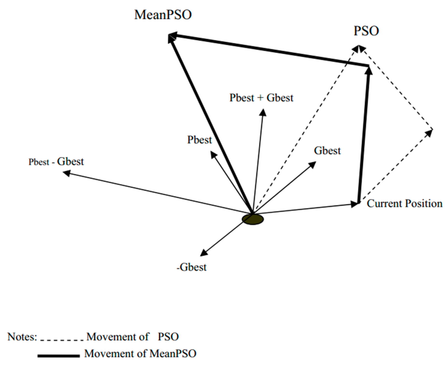
Deep et al. replaced the individual optimum and group optimum in the particle velocity update formula with the linear combination of the two; that is, $\frac{pbes{t}_{id}+gbes{t}_d}{2}$ and $\frac{pbes{t}_{id}-gbes{t}_d}{2}$ are used to replace pbest_id and gbest_d in the particle velocity update formula, respectively [40]. The study proposed a mean particle swarm optimization algorithm (MeanPSO) to increase the search space of particles. The second term of the particle velocity update formula in Equation (1) becomes $c_{1}ran{d}_1(\frac{pbes{t}_{id}+gbes{t}_d}{2}-x_{id}(t))$, which is responsible for attracting a particle’s current position towards the mean of the positive direction of the global best position (gbest) and the positive direction of its own best position (pbest). The third term of the particle velocity update formula in Equation (1) becomes $c_{2}ran{d}_2(\frac{pbes{t}_{id}-gbes{t}_d}{2}-x_{id}(t))$, which is responsible for attracting the current position of a particle to the mean of the positive direction of its own best position (pbest) and the negative direction of the global best position (−gbest). The relative position of the new positions generated by PSO and MeanPSO can be visualized in Figure 1.

Figure 1 comes from [40]. This study in [40] points out that the MeanPSO algorithm outperforms the PSO algorithm in terms of efficiency, accuracy, reliability, and robustness. Especially for large-sized problems, MeanPSO outperforms PSO. In addition, it can be seen from Figure 1 that the particle search interval in the MeanPSO algorithm is wider, which makes the algorithm more likely to search for the global optimal solution in the early stage of evolution. Liu proposed a hierarchical simplified particle swarm optimization algorithm with average dimension information (PHSPSO) [41]. The PHSPSO algorithm abandons the particle velocity update term in the PSO algorithm and introduces the concept of average dimension information, that is, the average value of all the dimension information of each particle. The calculation formula is shown in Equation (2). The PHSPSO algorithm decomposes the particle position update formula into three modes, namely, Equations (3)–(5).

$$P_{ad}(t)=\frac{1}{D}{\displaystyle \sum _{i=1}^D{x}_{id}(t)}$$

(2)

$$x_{id}(t+1)=w{x}_{id}(t)+c_1{r}_1(pbes{t}_{id}-x_{id}(t))$$

(3)

$$x_{id}(t+1)=w{x}_{id}(t)+c_2{r}_2(gbes{t}_d-x_{id}(t))$$

(4)

$$x_{id}(t+1)=w{x}_{id}(t)+c_3{r}_3(p_{ad}-x_{id}(t))$$

(5)

where Equation (3) contributes to the global development ability of the algorithm, Equation (4) contributes to the local exploration ability of the algorithm, and Equation (5) helps to improve the convergence speed of the algorithm. In the iterative process, the algorithm selects different patterns based on probability to update the particle position.

The work in [37] pointed out that using “x = x + v” to update the particle position helps to improve the local exploration ability of the algorithm, and ”x = wx + (1 − w)v” helps to improve the global development ability of the algorithm. In order to balance local development and global exploration, an adaptive position update mechanism is proposed. Using this mechanism, the particles can select the position update strategy according to the corresponding conditions to better balance the local exploration ability and the global development ability. The position update strategy of the adaptive strategy is expressed by Equation (6).

$$P_i=\frac{\mathit{exp}(fit(x_i(t)))}{\mathit{exp}\left(\frac{1}{N}{\displaystyle \sum _{i=1}^{N}fit(x_i(t))}\right)}$$

(6)

where fit(·) is the fitness value of the particle, and N is the number of particles in the population. In Equation (6), p_i denotes the ratio of the fitness value of the current particle to the average fitness value of all particles in the population. When the p_i value is greater than the random number, the fitness value of the current particle is much larger than the average fitness value of all particles in the population. At this time, “x = wx + (1 − w)v” should be used to update the particle position to enhance the global development ability of the algorithm. Otherwise, “x = x + v” is used to update the particle position to ensure the local exploration ability of the algorithm.

In order to improve the feasibility and effectiveness of the particle swarm optimization algorithm, Yang et al. introduced the evolution speed factor and aggregation factor. By analyzing these two parameters, the author proposed a dynamic change strategy of inertia weight based on the running state and evolution state [42]. Liang et al. proposed a comprehensive learning strategy of particle swarm optimization (CLPSO), which updated the speed by the historical best position of all other particles [43]. Adewumi et al. made a series of improvements to the inertia weight w and proposed the group success rate reduction inertia weight (SSRDIW) and the group success rate random inertia weight (SSRRIW). These two strategies improved the convergence speed, the global search ability, and the solution accuracy of the algorithm [44]. Particle swarm optimization belongs to the stochastic optimization method and is mainly driven by the random streams utilized in the search mechanism. Mingchang studied the influence of control randomness on the particle swarm search scheme by introducing three different pseudo-random number (PRN) allocation strategies. The results show that we can systematically select the appropriate PRN strategy and corresponding parameters to make the PSO algorithm more powerful and efficient [45].

According to the above discussion, this paper uses the improved particle swarm optimization algorithm (MPSO) to solve the optimal parameters of the Bayesian network model. The algorithm combines the ideas of [37,40,41], introduces the adaptive decision mechanism, and introduces the nonlinear inertia weight. The experimental results show that the algorithm is better than the traditional PSO algorithm.

This research accomplishes the following three things:

• Constructs a multilayer Bayesian network demand prediction model that considers demand volatility and time series correlation.
• Introduces a modified PSO algorithm (MPSO) for solving the maximum a posteriori estimates of parameters.
• Assesses the proposed approach’s performance via a thorough experimental evaluation.

Based on the above discussion, the motivation behind this research work is based on two arguments. First, Bayesian methods have been successful in many fields and predictive environments and are particularly promising and appealing when there are considerable changes in the data. Second, it is assumed that the demand and parameters obey the normal distribution, which has a conjugate prior. When the posterior distribution is derived, the maximum posterior is used to estimate the relevant parameters. Therefore, combining the BN with the PSO algorithm, we use the improved PSO algorithm to optimize the function form of the posterior distribution. This paper proposes a more general Bayesian network demand-forecasting model and designs a more novel solution method, which provides a new idea for demand forecasting in the supply chain.

The remainder of the paper is organized as follows. Section 2 introduces the proposed Bayesian network prediction model. In Section 3, we describe the solution algorithm of the model. Section 4 is dedicated to the experiment and the discussion of results. Conclusions and future work are put forward in Section 5.

2. Bayesian Network Model Construction

2.1. Problem Description and Assumptions

This section aims at how a specific enterprise in the supply chain node predicts the demand for products in a future period of time based on the historical sales data of products. In reality, the actual demand of consumers is not available due to the occurrence of situations such as stock-outs, so this paper equates the sales volume of goods with the actual demand of customers. Specifically, in this section, the following problem is considered: given the historical sales data of commodities, suppose that the demand quantity of commodities in the past T consecutive time points is 1, 2, …, T is y₁, y₂, …, y_T, make a relatively accurate prediction of the demand quantity of commodities in the future T + 1, T + 2, …, T + n, and finally, minimize the prediction error. The multilayer Bayesian network demand-forecasting model constructed in this paper considers the continuity and volatility of commodity demand in time series, and the flow chart of the forecasting plan is shown in Figure 2.

Assuming that the historical sales data of a certain product are known, the demand for a single product in the future period of time is forecasted, and the customer demand for the product at time t is recorded as y_T. Then, y_T represents the time series data, and there are time series characteristics. In addition, a hyperparameter layer is introduced on the middle layer to smooth the data fitting effect. Aiming at the volatility of product demand, the volatility factor γ and the correction factor β are introduced to better fit the data. Specifically, it is assumed that each variable has the following relationship with each other, and the probability graphical model is shown in Figure 3.

Assume that the variables in Figure 3 have the following relationships with each other:

• Assume that at any time t, the customer’s demand for goods satisfies the Gaussian distribution with mean value γ_tη_t + β and variance σ_y². The large fluctuation of the actual commodity data, namely, the change of the data on the time nodes before and after, shows a strong randomness. Therefore, it is assumed that the observations at different times are independent of each other. For the observation data y_t at any time, there is:

y_t ~ N(γ_tη_t + β, σ_y²)

(7)

where η_t represents the sequential characteristics of the customer demand for goods. γ_t represents the volatility factor, representing the volatility of customer demand for commodities, which often has a certain cyclical law. β is the correction factor.

2.

The hidden layer variable η_t at any time is only affected by the previous moment, η_t−1, and only affects the next moment, η_t+1. The hidden layer variable has the first-order Markov property on the time axis, which can be obtained:

$$P({\eta }_t|{\eta }_1,{\eta }_2,{\eta }_3,\cdots ,{\eta }_{t-1})=P({\eta }_t|{\eta }_{t-1})$$

(8)

Furthermore, taking into account the timing characteristics of the number of customers’ demand for goods, it is assumed that the hidden layer variables at each time point obey the following first-order autoregressive model:

$${\eta }_t=\{\begin{array}{cc}\mu +{\epsilon }_t\hfill & t=1\\ \mu +\varphi \left({\eta }_{t-1}-\mu \right)\hfill & t>1\end{array}$$

(9)

where μ∈R represents the long-term mean value of η_t; −1 < ϕ < 1 represents the rate of autoregression; ε_t represents the noise term of autoregression; and ${\epsilon }_t\sim N(0,1)$.

3.

It can be seen from the probability diagram model in Figure 3 that the fluctuation factor γ_t directly acts on the demand data y_t. In real life, consumers have a certain periodicity in their purchase behavior of commodities, whether online or in physical stores. In addition, some commodities have a certain service cycle and life, so we assume that the fluctuation factor γ_t has periodicity and the period is H. That is, the relationship between each γ_t should satisfy the following:

γ_i+H = γ_i (i = 0, 1, 2, …)

(10)

γ ~ N(0, σ_γ²)

(11)

According to this assumption, for any time γ_t, it not only affects the demand data y_t at the same time, but also affects y_t+H, …, y_t+nH (n = 1, 2, …).

4.

The correction factor β as well as hyperparameters μ and ϕ obey normal distribution independently.

β ~ N(0, σ_β²)

(12)

μ ~ N(m₀, σ_μ²)

(13)

ϕ ~ N(0, σ_ϕ²)

(14)

where m₀ is defined as the mean of customer demand for the target item at all historical points in time, and since ϕ∈(−1,1), according to the principle of “σ” and “3σ” of normal distribution, the value of σ_ϕ² is limited to [0.5,1].

2.2. Parameter Estimation

This section mainly discusses how to estimate the model parameters η, γ, β, μ, and ϕ in the case of given historical demand data y = (y₁, y₂, …, y_T) of a particular product.

The maximum posterior probability estimation is used to estimate the above parameters, and the problem can be expressed as Equation (15).

$$\left\{\widehat{\eta },\widehat{\gamma },\widehat{\beta },\widehat{\mu },\widehat{\varphi }\right\}=\underset{\eta ,\gamma ,\beta ,\mu ,\varphi }{\mathit{arg}\mathit{max}}P({\eta }_{1:T},{\gamma }_{1:T},\beta ,\mu ,\varphi )$$

(15)

Here, let us think of P as a function of the variables η, γ, β, μ, and ϕ.

In the case of unknown parameters β, μ, ϕ, η, and γ, given the historical demand data of known customers with a quantity of T, according to Bayes’ theorem, they can be deduced as follows:

$$\begin{array}{cc}\hfill P\left({\eta }_{1:T},{\gamma }_{1:T},\beta ,\mu ,\varphi |y_{1:T}\right)& =\frac{P\left({\eta }_{1:T},{\gamma }_{1:T},\beta ,\mu ,\varphi ,y_{1:T}\right)}{P\left(y_{1:T}\right)}\hfill \\ & \propto P\left({\eta }_{1:T},{\gamma }_{1:T},\beta ,\mu ,\varphi ,y_{1:T}\right)\hfill \\ & =P\left(y_{1:T}|{\eta }_{1:T},{\gamma }_{1:T},\beta ,\mu ,\varphi \right)P\left({\eta }_{1:T},{\gamma }_{1:T},\beta ,\mu ,\varphi \right)\hfill \end{array}$$

(16)

Furthermore, according to the relationships between the variables in Figure 3, it can be obtained that the distribution on the right side of Equation (16) has the following relationship:

$$P\left(y_{1:T}|{\eta }_{1:T},{\gamma }_{1:T},\beta ,\mu ,\varphi \right)=P\left(y_{1:T}|{\eta }_{1:T},{\gamma }_{1:T},\beta \right)={\displaystyle \prod _{t=1}^{T}P}\left(y_t|{\eta }_t,{\gamma }_t,\beta \right)$$

$$P\left({\eta }_{1:T},{\gamma }_{1:T},\beta ,\mu ,\varphi \right)=P({\eta }_1|\mu ,\varphi ){\displaystyle \prod _{t=2}^{T}P({\eta }_t|{\eta }_{t-1},\mu ,\varphi )}\times {\displaystyle \prod _{i=1}^{H}P({\gamma }_i)}\times P(\beta )\times P(\mu )\times P(\varphi )$$

(17)

where the periodic factor satisfies the periodic assumption of Equation (10), that is, $P({\gamma }_{1:T})={\displaystyle \prod _{i=1}^{H}P({\gamma }_i)}$. According to the assumption of the Equation (9) and taking logarithms at both ends of the equation, the result is recorded as l. Furthermore, according to the probability density function of the distribution obeyed by the parameters, Equation (18) is finally obtained.

$$\begin{array}{cc}\hfill l=& -\frac{1}{{\sigma }_{\mathrm{y}}{}^2}{\displaystyle \sum _{t=1}^T{(yt-{\eta }_t{\gamma }_t-\beta )}^2}-{({\eta }_1-\mu -\varphi ({\eta }_2-\mu ))}^2+\frac{T-2}{2}\log (1+{\varphi }^2)-\hfill \\ & {\displaystyle \sum _{t=2}^{T-1}\left[{({\eta }_t-\mu -\varphi ({\eta }_{t-1}+{\eta }_{t+1}-2\mu ))}^2(1+{\varphi }^2)\right]}-{({\eta }_T-\mu -\varphi ({\eta }_{T-1}-\mu ))}^2\hfill \\ & -\frac{1}{{\sigma }_{\gamma }{}^2}{\displaystyle \sum _{i=1}^H{\gamma }_i{}^2}-\frac{1}{{\sigma }_{\beta }{}^2}{\beta }^2-\frac{1}{{\sigma }_{\mu }{}^2}{(\mu -m_0)}^2-\frac{1}{{\sigma }_{\varphi }{}^2}{\varphi }^2+C\hfill \end{array}$$

(18)

where C is a constant, which does not affect the result, and is omitted below. If π = −l, Equation (18) is equivalent to:

$$\left\{\widehat{\eta },\widehat{\gamma },\widehat{\beta },\widehat{\mu },\widehat{\varphi }\right\}=\underset{\eta ,\gamma ,\beta ,\mu ,\varphi }{\mathit{arg}\mathit{min}}\pi ({\eta }_{1:T},{\gamma }_{1:T},\beta ,\mu ,\varphi )$$

(19)

The formula for π(η, γ, β, μ, ϕ) can be expressed as follows:

$$\begin{array}{cc}\hfill \pi =& \frac{1}{{\sigma }_{\mathrm{y}}{}^2}{\displaystyle \sum _{t=1}^T{(yt-{\eta }_t{\gamma }_t-\beta )}^2}+{({\eta }_1-\mu -\varphi ({\eta }_2-\mu ))}^2-\frac{T-2}{2}\log (1+{\varphi }^2)+\hfill \\ & {\displaystyle \sum _{t=2}^{T-1}\left[{({\eta }_t-\mu -\varphi ({\eta }_{t-1}+{\eta }_{t+1}-2\mu ))}^2(1+{\varphi }^2)\right]}+{({\eta }_T-\mu -\varphi ({\eta }_{T-1}-\mu ))}^2\hfill \\ & +\frac{1}{{\sigma }_{\gamma }{}^2}{\displaystyle \sum _{i=1}^H{\gamma }_i{}^2}+\frac{1}{{\sigma }_{\beta }{}^2}{\beta }^2+\frac{1}{{\sigma }_{\mu }{}^2}{(\mu -m_0)}^2+\frac{1}{{\sigma }_{\varphi }{}^2}{\varphi }^2\hfill \end{array}$$

(20)

3. Model Solving

3.1. MPSO Algorithm Design

This section uses a particle update strategy that introduces an adaptive decision mechanism and a particle swarm optimization algorithm (MPSO) based on Logistic mapping to update the inertia weight and solve the above model. Specifically, in the t + 1 iteration, the particles update the velocity and position according to Equations (21) and (22).

$$\{\begin{array}{c}{v}_{id}(t+1)=w{v}_{id}(t)+c_1{r}_1(\frac{pbes{t}_{id}+gbes{t}_d}{2}-x_{id}(t))+c_2{r}_2(\frac{pbes{t}_{id}-gbes{t}_d}{2}-x_{id}(t))\\ x_{id}(t+1)=w{x}_{id}(t)+(1-w)v_{id}(t+1)\end{array}$$

(21)

$$\{\begin{array}{c}{v}_{id}(t+1)=w{v}_{id}(t)+c_1{r}_1(p_{ad}-x_{id}(t))+c_2{r}_2(gbes{t}_d-x_{id}(t))\\ x_{id}(t+1)=x_{id}(t)+v_{id}(t+1)\end{array}$$

(22)

Equation (21) introduces the speed update strategy in [40], and the position update strategy adopts “x = wx + (1 − w)v” so as to improve the global development ability of particles in the early stage of the search. In Equation (22), the position update strategy of “x = x + v” is used to improve the local exploration ability of particles. Combined with the idea of [41], the average dimension information pad of particles is introduced into the velocity update formula to improve the local search efficiency of particles. The calculation formula of p_ad is shown in Equation (2).

The MPSO algorithm adopts the adaptive decision mechanism in [37], and the calculation formula of P_i is shown in Equation (6). P_i represents the adaptive decision condition of the particle position and velocity update strategy. When P_i is greater than δ, the fitness value of the current particle is greater than the average fitness value of all particles in the population. The current particle distribution is relatively dispersed, and the algorithm is in the initial search stage. In this case, Equation (21) should be used to update the velocity and position of particles. Equation (21) introduces a linear combination of individual optimization and group optimization in the velocity update term, which makes the particle search space wider and improves the possibility of finding the global optimal solution. The position update formula helps to improve the global search ability of the algorithm. When P_i is less than δ, the fitness value of the current particle is close to the average fitness value of all particles in the population, indicating that the particle distribution is relatively concentrated. The Equation (22) should be used to update the particle velocity and position. In the MPSO algorithm, the δ value is set to 0.6.

As a kind of nonlinear mapping, chaotic mapping has been widely used in evolutionary computation because of the good randomness and spatial ergodicity of the chaotic sequences generated by it. Among them, Logistic mapping is widely used, which can generate random numbers between [0,1]. Equation (23) defines a Logistic mapping, and w is defined as in Equation (24):

$$r(t+1)=4r(t)(1-r(t)),r(0)=rand,r(0)\notin \left\{0,0.25,0.5,0.75,1\right\}$$

(23)

$$w(t)=r(t)w_{\min }+\frac{(w_{\max }-w_{\min })t}{T_{\max }}$$

(24)

where w_max = 0.9, w_min = 0.4; and r(t) is a random number generated iteratively by Equation (23). The corresponding simulation diagram is shown in Figure 4. It can be seen from Figure 4 that the value of inertia weight w fluctuates strongly throughout the iteration process. As the number of iterations changes, this nonlinear inertia weight has a strong simulation fitting ability. In addition, the w with strong volatility makes the particles more random in the update process and less likely to fall into the local optimum [46].

The implementation steps of the MPSO algorithm are as follows:

3.2. Model Prediction Process

The current customer demand data are y₁, y₂, ..., y_T. The hidden layer parameter ${\widehat{\eta }}_1,{\widehat{\eta }}_2,\mathrm{...},{\widehat{\eta }}_T$ and the hyper-parameter layers $\widehat{\gamma },\widehat{\beta },\widehat{\mu },\widehat{\varphi }$ corresponding to y at each moment are obtained by using Algorithm 1. According to Equation (9), the estimation of the next hidden layer parameter η_T+1 can be obtained, and then, according to Equation (8), the estimation of the next requirement y_T+1 can be obtained. Repeat this process, and “${\widehat{\eta }}_{T+1}\to {\widehat{y}}_{T+1}\to {\widehat{\eta }}_{T+2}\to {\widehat{y}}_{T+2}\mathrm{...}$” can be obtained in turn. The specific prediction process is shown in Algorithm 2.

Algorithm 1 Parameter optimization steps

Input: Customer historical demand data y = (y1, y2, …, yT); objective function Equation (20); decision variables: η ∈ [0, max(yt)], γ ∈ [0, 3σγ], β ∈ [−3σβ, 3σβ], μ ∈ [0, m0 + 3σμ], ϕ ∈ (−1, 1); the adjustment parameters σy2, σγ2, σβ2, σμ2, σϕ2 of objective function; periodic factor H; the value of δ

Output: Model parameter estimates $\widehat{\eta },\widehat{\gamma },\widehat{\beta },\widehat{\mu },\widehat{\varphi }$

1. The initial value of model parameters is generated according to (γ1, …, γT) ~ N(0, σγ2), μ~N(m0, σμ2), β~N(0, σβ2), and ϕ~N(0, σϕ2), and the initial value of ηt is generated according to Equation (9).

2. Initialization parameters Tmax, N, c1, c2, and w as well as particle position and velocity;

3. For i: = 1 to Tmax do;

4.  Evaluate particles to get pbest and gbest;

5.  Update inertia weight w;

6.  If Pi > δ do;

7.   Adopt the update strategy of Equation (21);

8.  Else do;

9.   Adopt the update strategy of Equation (22);

10.  End if;

11. End for;

12.Output $\widehat{\eta },\widehat{\gamma },\widehat{\beta },\widehat{\mu },\widehat{\varphi }$.

Algorithm 2 Prediction procedure

Input: Historical demand data y = (y1, y2, …, yT); the fitting parameters $\widehat{\eta },\widehat{\gamma },\widehat{\beta },\widehat{\mu },\widehat{\varphi }$ of the model; the sequence length n to be predicted

Output: Future demand forecast sequence (yT+1, yT+2, …, yT+n)

1. For i: = 1 to n do;

2.  Compute ηT+i according to Equation (9), update inertia weight w;

3.  $y_{T+i}={\widehat{\gamma }}_{T+i}{\eta }_{T+i}+\widehat{\beta }$;

4. End for;

5. Output (yT+1, yT+2, …, yT+n).

4. Experiment

4.1. Data Description Statistics

In this section, based on the prediction model and solution method proposed in this paper, the dataset of the “DataFountain” platform is used as a sample to predict the commodity demand of an e-commerce enterprise for the next week. In this paper, the three attributes of sku_id, goods_num, and data_date in this dataset are used to randomly select commodities with sku_id as “SK4taRSU”, “SKlLr87U”, and “SKJCqIoN” as experimental datasets DS-1, DS-2, and DS-3. In order to verify the accuracy of the prediction results, the product sales volume from 1 March 2017 to 29 October 2017 is used as the training data, and the product sales volume from 30 October 2017 to 5 November 2017 is used as the test set for verification. The online retail dataset DS-4 was also selected from UCI, which includes transactions from a UK e-commerce company for 374 days from 1 December 2010 to 9 December 2011. Because of Christmas and the New Year, there are 11 consecutive days of blank records in the dataset. Therefore, after removing the blank record, this paper selected the commodity with the most complete sales record and summarized the sales quantity by week to get the data of 51 weeks for the experiment. In addition, this paper also features the sales data DS-5 and DS-6 of two kinds of commodities on an e-commerce platform for the experiment. The sequence diagrams of the DS-1~6 datasets are shown in Figure 5:

As can be seen from the time series graphs, not only the fluctuations of adjacent time nodes are large, but also the overall volatility of these six datasets is strong, which poses a great challenge to the demand-forecasting problem.

Table 1. Description statistics for datasets DS-1 to 6.

Dataset	DS-1	DS-2	DS-3	DS-4	DS-5	DS-6
Unit of time	day	day	day	week	day	day
The length	250	250	250	51	611	611
The mean	32.83	168.11	61.02	449.22	3.50	2.00
Standard deviation	26.79	75.98	48.31	481.19	4.01	2.56
Dispersion coefficient	0.82	0.45	0.79	1.07	1.14	1.31

summarizes some statistical features of DS-1 to 6. It can be seen from Table 1 that the dispersion coefficients of these six datasets are very high, and the fluctuations are quite dramatic, which is consistent with the results of the time series diagram. Therefore, it is reasonable to add the volatility factor γ to the model established in this paper.

4.2. Results of Measurement

In terms of the measurement results, RMSE (Root Mean Square Error, RMSE) and MAPE (Mean Absolute Percentage Error) are used as the evaluation indicators of the algorithm proposed in this chapter. RMSE is used to measure the absolute error between the predicted value and the actual value, and MAPE reflects the relative size of the error between the predicted value and the actual value. The smaller the value of the above two evaluation indicators, the higher the prediction accuracy. Suppose at points 1, 2, 3, …, n, the actual quantity of the customer demand for goods is $y_1, y_2, y_3, \dots , y_n$. The corresponding results predicted by the algorithm are ${\widehat{y}}_1, {\widehat{y}}_2, {\widehat{y}}_3, \dots , {\widehat{y}}_n$. The calculation formulas of RMSE and MAPE are as follows:

$$RMSE=\sqrt{\frac{{\displaystyle \sum _{i=1}^n{(\widehat{y_i}-y_i)}^2}}{n}}$$

(25)

$$MAPE=\frac{1}{n}{\displaystyle \sum _{i=1}^n\left|\frac{y_i-\widehat{y_i}}{{\mathrm{y}}_{\mathrm{i}}}\right|}$$

(26)

4.3. Parameter Adjustment of the Model

This subsection discusses the parameter tuning process of the model. There are six tuning parameters in the model, among which σ_μ and σ_ϕ act on the hyperparametric variables μ and ϕ, and σ_γ and σ_β act on the variables γ and β. These parameters are mainly used to smooth the estimation results of the above variables. Empirically, the setting of these parameters does not have a significant effect on the prediction results. Therefore, for the convenience of adjustment, set these parameters as 1, and let α be σ_y⁻².

Different from the above parameters, the parameters α and H directly act on the observation data y, so the selection of α and H has a direct impact on the performance of the model. This work focus on the regulation of H and parameter α. For datasets DS-1–3, the product sales volumes from 1 March 2017 to 29 October 2017 are used as the training data, and the product sales volumes from 30 October 2017 to 5 November 2017 are used as the test set to adjust parameter H. The first 90% of the data in datasets DS-4–6 were selected as training data for model fitting, and the last 10% of the data as model validation.

4.3.1. Adjustment of Parameter H

During the adjustment of parameter H, the training set in the dataset traverses all values of H ∈ [1,30]. Fixed σ_y is the variance of the training set used for fitting, and RMSE is used as the measurement standard. The experimental results are shown as follows:

Based on the results in Figure 6, it can be seen that the variation trend of the value of period H presents different characteristics in different datasets. Therefore, it is further verified that the selection of the period H value plays a crucial role in the prediction performance of the model.

Parameter H is the periodic factor of the volatility factor γ_t in the model. If the sample data are sensitive to parameter H, it indicates that the fluctuation of the sample data is regular, which may be because the customer’s behavior of purchasing the product usually has certain regularity. Therefore, choosing an appropriate period H has a great influence on the accuracy of prediction. If the variation range of prediction error is small with the change of H, then H is generally selected within a reasonable range, and the prediction accuracy of the algorithm can be guaranteed.

Finally, according to Figure 6, the value of H on each dataset can be obtained, as shown in

Table 2. Set H on DS-1 to 6.

	DS-1	DS-2	DS-3	DS-4	DS-5	DS-6
H	9	16	17	8	17	28

:

4.3.2. Adjustment of Parameter α

This section discusses the tuning of the parameter α. Similar to the above section, each training set of DS-1 to 6 is used to verify the possible value of α. Similar to the adjustment process of parameter H, in each experiment, the work randomly selected the first 90% of the data from the training dataset for model fitting and the remaining 10% as model validation. The range of α is defined in the set {2⁻²⁰, 2⁻¹⁹, …, 2⁻¹}, the value of H is shown in Table 2, RMSE is taken as the measurement standard, and the experimental results are shown in Figure 7:

According to Figure 7, the value of α on each dataset can be obtained, as listed in

Table 3. Set α on DS-1 to 6 (α = σ_y⁻²).

	DS-1	DS-2	DS-3	DS-4	DS-5	DS-6
α	2−11	2−18	2−16	2−19	2−3	2−4

:

4.4. Comparative Analysis of Prediction Results

In order to verify the effectiveness of the model and algorithm, firstly, this section selects four classic test functions and compares the MPSO algorithm with the standard PSO algorithm. The relevant descriptions of the four test functions are shown in

Table 4. Benchmark functions.

Name	Benchmark Functions	Range	fopt
Schwefel 2.22	f1(x) = ${\displaystyle \sum _{i=1}^D\left|x_i\right|}+{\displaystyle \prod _{i=1}^D\left|x_i\right|}$	[−10,10]	0
Ackley	f2(x) = $-20\mathit{exp}(-0.2\sqrt{\frac{1}{D}{\displaystyle \sum _{i=1}^D{(x_i)}^2}})-\mathit{exp}(\frac{1}{D}{\displaystyle \sum _{i=1}^D\mathit{cos}(2\pi x_i)})+20+e$	[−32,32]	0
Griewank	f3(x) = $\frac{1}{4000}{\displaystyle \sum _{i=1}^D{x}_i{}^2}-{\displaystyle \prod _{i=1}^D\mathit{cos}(\frac{x_i}{\sqrt{i}})}+1$	[−600,600]	0
Rastrigin	f4(x) = ${\displaystyle \sum _{i=1}^D\left[x_i{}^2-10\mathit{cos}(2\pi x_i)+10\right]}$	[−5.12,5.12]	0

. Secondly, this section compares the prediction effect of the proposed method on the above six datasets with the prediction effect of the ARIMA method.

The population size is set to N = 100, the maximum number of iterations T_max = 1000, and the variable dimension D = 30. The two algorithms run 50 times independently, and the average and standard deviation of the results of 50 runs are recorded to evaluate the performance of the algorithm. The results are shown in

Table 5. Comparison of operation results.

Function	Index	MPSO	PSO
f1	Mean	1.1605 × 10−34	2.2009 × 10−4
	Std	7.5208 × 10−34	3.4046 × 10−4
f2	Mean	4.4409 × 10−16	2.2597 × 10−5
	Std	0	3.4402 × 10−5
f3	Mean	0	8.7885 × 10−7
	Std	0	2.1279 × 10−6
f4	Mean	0	6.3885 × 10−4
	Std	0	4.5000 × 10−3

.

It can be seen from Table 5 that the solution accuracy of the MPSO algorithm is better than that of classical PSO algorithm. Furthermore, this section uses the classical PSO algorithm and the MPSO algorithm to solve the parameters of the Bayesian network model and uses the solution results for prediction. In terms of the time complexity of the algorithm, the time complexity of the standard PSO algorithm is O(nmD), where n is the number of particles, m is the number of iterations of the algorithm, and D is the dimension of the problem. The MPSO algorithm uses Equations (21) and (22) to update the particle velocity and position, which is only one more adaptive decision than the standard PSO algorithm. The improved strategy does not increase the time complexity of the algorithm. Through the above experiments and analysis, the MPSO algorithm has better performance in solving multimodal function problems with higher dimensions. Next, we apply the algorithm to solve the actual prediction problem and further prove that the algorithm is better than the PSO algorithm through the prediction effect.

In the process of model prediction, other parameters also have an impact on the data fitting and solving efficiency. Through several experiments, the values of other parameters are shown in

Table 6. MPSO parameter settings.

Datasets	Variance Parameters				MPSO Parameters			Prediction Length
	σγ−2	σβ−2	σμ−2	σϕ−2	c1	c2	δ	n
DS-1	0.01	0.001	0.01	0.5	1.5	1.5	0.6	7
DS-2	0.01	0.001	0.01	0.5	1.5	1.5	0.6	7
DS-3	1	1	1	1	1.5	1.5	0.6	7
DS-4	1	1	1	1	1.5	1.5	0.6	5
DS-5	0.1	100	1	0.5	1.5	1.5	0.6	61
DS-6	0.1	100	100	0.5	1.5	1.5	0.6	61

:

In the process of model prediction, different initialization parameters may have an impact on the prediction results, so the experiment was repeated 10 times for each dataset, and the final result was taken as the average of the 10 experiments. The prediction results are summarized as shown in

Table 7. The RMSE value of the prediction result.

The Dataset	ARIMA	PSO	MPSO
DS-1	9.4635	7.8649	6.7964
DS-2	11.7463	5.9422	5.0250
DS-3	11.8518	10.5616	9.9798
DS-4	259.9827	105.4191	98.6192
DS-5	5.7647	5.6727	5.6445
DS-6	3.3200	3.2255	3.2073

:

In order to better verify the effectiveness of the model and algorithm, datasets DS-1, DS-2, DS-3, DS-5, and DS-6 were selected to conduct experiments in the predicted length of 10, 20, and 30 days, respectively. Due to the relatively small amount of data in dataset DS-4, this experiment was not carried out on it. In addition, it can be seen from Figure 5 that the demand for datasets DS-5 and DS-6 fluctuates greatly, and there are many zero values. Hence, we use the Croston method to predict these two datasets.

When the real value is 0, the prediction error evaluated by the MAPE index will approach infinity, so the results measured by the MAPE index are invalid. Therefore, when MAPE is used as the evaluation index in this paper, when the actual value is 0, the mean value of the actual value in the sample is used for correction. MAPE reflects the relative size of the error between the predicted value and the actual value, and a smaller value of MAPE indicates a higher accuracy of the prediction. The experimental results are shown in

Table 8. Prediction result statistics.

Dataset	RMSE	MAPE	RMSE	MAPE	RMSE	MAPE
	DS-1
n	10		20		30
ARIMA	13.0137	0.3533	10.1142	0.2580	9.4370	0.2608
Standard PSO	10.0647	0.2899	8.6060	0.2409	8.4051	0.2478
MPSO	9.3224	0.2647	7.9575	0.2301	8.1840	0.2363
Dataset	DS-2
n	10		20		30
ARIMA	18.8025	0.5415	32.5209	0.6418	30.3403	0.5449
Standard PSO	9.2079	0.2614	29.4158	0.3723	32.0604	0.3942
MPSO	8.6293	0.2413	28.5674	0.3558	31.3899	0.3846
Dataset	DS-3
n	10		20		30
ARIMA	10.6941	0.4448	14.3582	0.4600	14.2508	0.3867
Standard PSO	7.7633	0.3977	13.6170	0.4428	13.9329	0.3853
MPSO	7.5219	0.4128	13.4165	0.4377	13.9712	0.3793
Dataset	DS-5
n	10		20		30
ARIMA	5.4625	1.3020	8.8338	1.2279	7.4327	1.0158
Crotson	5.0750	1.0128	9.3064	1.2305	7.8490	1.1819
Standard PSO	3.5871	0.3868	8.8211	0.5093	7.0309	0.5416
MPSO	3.5463	0.3615	8.7226	0.5015	6.8086	0.5369
Dataset	DS-6
n	10		20		30
ARIMA	1.6196	0.4202	4.6320	0.5180	3.8601	0.5088
Crotson	1.5388	0.5410	4.5941	0.5579	4.4414	0.5331
Standard PSO	1.5187	0.3946	4.5995	0.4835	3.8314	0.4662
MPSO	1.4923	0.3560	4.5989	0.4828	3.9761	0.4612

:

In terms of prediction methods, the Bayesian network prediction model shows better prediction results as a whole. When the prediction length of the DS-2 dataset is 30, the RMSE indicator is higher, but the MAPE indicator performs better. In terms of the solving algorithm, according to the results of the benchmark function in Table 5, the accuracy of the MPSO algorithm is better than that of the PSO algorithm. According to the prediction results in Table 8, the MPSO algorithm is better than the PSO algorithm in solving the Bayesian network prediction model.

As seen in Table 7 and Table 8, the multilayer Bayesian network prediction model has achieved good prediction results, which indicates that the model is more effective in the application of demand forecasting with large fluctuations. In addition, on the datasets DS-5 and DS-6, the data not only fluctuate greatly, but also show intervals. Hence, we add the results of the Croston method to predict the datasets DS-5 and DS-6 in Table 8. It can be seen from the results that the proposed method has a better prediction effect than the Croston method.

In this paper, a more general Bayesian network demand-forecasting model is proposed. The model introduces a fluctuation factor on the basis of hidden layer variables, which can better adapt to the fluctuation of data. In Section 4, we selected the data with strong volatility and verified the validity of the model through experiments. Many studies have shown that the Bayesian method has better performance when the data fluctuation is strong. The Bayesian method needs to introduce a suitable prior distribution. The model assumes that the demand and parameters obey the normal distribution, which simplifies the calculation formula of the maximum posterior estimation. In this paper, the BN is combined with PSO, and the improved PSO algorithm is used to solve the maximum posteriori estimation function. The experimental results show that the improved MPSO algorithm is superior to the PSO algorithm in solving accuracy.

5. Conclusions

Nowadays, product substitutability is enhanced, and customized products are becoming a trend, which makes product demand show strong volatility. Considering the time series correlation and strong volatility of demand data, this study introduces hidden layer variables and volatility factors into the multilayer Bayesian network model. According to the relevant theoretical knowledge of Bayesian statistics, the parameters of the model are estimated by the maximum posterior estimation method. Due to the large number of model parameters and the complex objective function, this work improves the standard PSO algorithm. The algorithm introduces the particle update strategy of the adaptive decision mechanism and adopts nonlinear inertia weight. The effectiveness of the model and algorithm is proved by comparative experiments.

Accurate prediction of terminal customer demand is the basis for formulating production planning, inventory strategy, facility planning, and distribution strategy in the supply chain. The demand-forecasting model proposed in this paper provides a new idea for demand forecasting in the supply chain. In particular, with the in-depth development of the industrial internet, improving the accuracy of customer demand forecasting in the supply chain is of great practical significance for enterprises to improve the efficiency of production resource allocation.

This study does not consider the specific factors affecting demand and the correlation between different products. The factors affecting product demand and the correlation between products need to be quantified according to the actual situation. The correction factors in the multilayer Bayesian network model can be replaced by quantitative influencing factors. In this case, the model is more complex. The model proposed in this paper has strong applicability when it is difficult to quantify the factors affecting demand or impossible to quantify the influencing factors. In addition, ways to further expand the proposed model and then study how to make the optimal production plan, inventory, and distribution plan will be the focus of future attention.

References

1. Euromonitor International. Top 10 Global Consumption Trends 2020 [EB/OL]. Available online: https://go.euromonitor.com/white -paper -EC-2020-Top-10-Global-Consumer-Trends (accessed on 10 March 2020).
2. Seeger, M.W.; Salinas, D.; Flunkert, V. Bayesian intermittent demand forecasting for large inventories. In Proceedings of the 30th Annual Conference on Neural Information Processing Systems (NIPS 2016), Barcelona, Spain, 4–9 December 2016. [Google Scholar]
3. Yavuz, A.; Sukran, K.; Peter, S. A decision support framework for global supply chain modelling: An assessment of the impact of demand, supply and lead-time uncertainties on performance. Int. J. Prod. Res. 2010, 48, 3245–3268. [Google Scholar]
4. Fu, W.; Chien, C.-F. UNISON data-driven intermittent demand forecast framework to empower supply chain resilience and an empirical study in electronics distribution. Comput. Ind. Eng. 2019, 135, 940–949. [Google Scholar] [CrossRef]
5. Fildes, R.; Kingsman, B. Incorporating demand uncertainty and forecast error in supply chain planning models. J. Oper. Res. Soc. 2011, 62, 483–500. [Google Scholar] [CrossRef]
6. Wan, X.; Sanders, N.R. The negative impact of product variety: Forecast bias, inventory levels, and the role of vertical integration. Int. J. Prod. Econ. 2017, 186, 123–131. [Google Scholar] [CrossRef]
7. Chien, C.-F.; Lin, Y.-S.; Lin, S.-K. Deep reinforcement learning for selecting demand forecast models to empower Industry 3.5 and an empirical study for a semiconductor component distributor. Int. J. Prod. Res. 2020, 58, 2784–2804. [Google Scholar] [CrossRef]
8. Geurts, M.; Box, G.E.P.; Jenkins, G.M. Time series analysis: Forecasting and control. J. Mark. Res. 1977, 14, 269. [Google Scholar] [CrossRef]
9. Chalabi, H.; Douri, Y.; Lundberg, J. Time Series Forecasting using ARIMA Model: A Case Study of Mining Face Drilling Rig. In The Twelfth International Conference on Advanced Engineering Computing and Applications in Sciences; International Academy, Research and Industry Association (IARIA): Wilmington, NC, USA, 2018. [Google Scholar]
10. Tseng, F.M.; Tzeng, G.H. A fuzzy seasonal ARIMA model for forecasting. Fuzzy Set Syst. 2002, 126, 367–376. [Google Scholar] [CrossRef]
11. Makoni, T.; Chikobvu, D. Modelling tourism demand volatility using a seasonal autoregressive integrated moving average autoregressive conditional heteroscedasticity model for Victoria Falls Rainforest arrivals in Zimbabwe. JEFS 2018, 11, 1–9. [Google Scholar] [CrossRef]
12. Blázquez-García, A.; Conde, A.; Milo, A. Short-term office building elevator energy consumption forecast using SARIMA. J. Build Perform Simu. 2020, 13, 69–78. [Google Scholar] [CrossRef]
13. Khashei, M.; Bijari, M.; Hejazi, S.R. Combining seasonal ARIMA models with computational intelligence techniques for time series forecasting. Soft Comput. 2012, 16, 1091–1105. [Google Scholar] [CrossRef]
14. Singh, P.; Dhiman, G. A hybrid fuzzy time series forecasting model based on granular computing and bio-inspired optimization approaches. J. Comput. Sci.-Neth. 2018, 27, 370–385. [Google Scholar] [CrossRef]
15. Egrioglu, E.; Bas, E.; Yolcu, O.C. Intuitionistic time series fuzzy inference system. Eng. Appl. Artif. Intel. 2019, 82, 175–183. [Google Scholar] [CrossRef]
16. Tratar, L.F.; Mojškerc, B.; Toman, A. Demand forecasting with four-parameter exponential smoothing. Int. J. Prod. Econ. 2016, 181, 162–173. [Google Scholar] [CrossRef]
17. Sbrana, G.; Silvestrini, A. Random switching exponential smoothing: A new estimation approach. Int. J. Prod. Econ. 2019, 211, 211–220. [Google Scholar] [CrossRef]
18. Mahajan, S.; Chen, L.J.; Tsai, T.C. Short-term PM2.5 forecasting using exponential smoothing method: A comparative analysis. Sensors 2018, 18, 3223. [Google Scholar] [CrossRef] [PubMed]
19. Omar, H.; Klibi, W.; Babai, M.Z. Basket data-driven approach for omnichannel demand forecasting. IJPE 2023, 257, 108748. [Google Scholar] [CrossRef]
20. Winters, P.R. Forecasting Sales by Exponentially Weighted Moving Averages. Manag. Sci. 1960, 6, 324–342. [Google Scholar] [CrossRef]
21. Johnston, F.R.; Boylan, J.E. Forecasting for items with intermittent demand. J. Oper. Res. Soc. 1996, 47, 113–121. [Google Scholar] [CrossRef]
22. Croston, J.D. Forecasting and Stock Control for Intermittent Demands. J. Oper. Res. Soc. 1972, 23, 289–303. [Google Scholar] [CrossRef]
23. Nambiar, M.; Simchi-Levi, D.; Wang, H. Dynamic learning and pricing with model misspecification. Manag. Sci. 2019, 65, 4980–5000. [Google Scholar] [CrossRef]
24. Hong, L.; Martin, R. Model misspecification, Bayesian versus credibility estimation, and Gibbs posteriors. Scand. Actuar. J 2020, 2020, 634–649. [Google Scholar] [CrossRef]
25. Frazier, D.T.; Robert, C.P.; Rousseau, J. Model misspecification in approximate Bayesian computation: Consequences and diagnostics. J. R. Stat. Soc. B. 2020, 82, 421–444. [Google Scholar] [CrossRef]
26. Babai, M.Z.; Chen, H.; Syntetos, A.A. A compound-Poisson Bayesian approach for spare parts inventory forecasting. IJPE 2021, 232, 107954. [Google Scholar] [CrossRef]
27. Snyder, R.D.; Keith, O.; Adrian, B. Forecasting the intermittent demand for slow-moving inventories: A modelling approach. Int. J. Forecast. 2012, 28, 485–496. [Google Scholar] [CrossRef]
28. Chapados, N. Effective Bayesian Modeling of Groups of Related Count Time Series. In Proceedings of the 31st International Conference on Machine Learning, Beijing, China, 21–26 June 2014. [Google Scholar]
29. Kon Kam King, G.; Canale, A.; Ruggiero, M. Bayesian functional forecasting with locally-autoregressive dependent processes. Bayesian Anal. 2019, 14, 1121–1141. [Google Scholar] [CrossRef]
30. Ye, Y.; Lu, Y.; Robinson, P. An empirical Bayes approach to incorporating demand intermittency and irregularity into inventory control. Eur. J. Oper. Res. 2022, 303, 255–272. [Google Scholar] [CrossRef]
31. Eskafi, M.; Kowsari, M.; Dastgheib, A. A model for port throughput forecasting using Bayesian estimation. Marit. Econ. Logist. 2021, 23, 348–368. [Google Scholar] [CrossRef]
32. Eskafi, M.; Kowsari, M.; Dastgheib, A. Mutual information analysis of the factors influencing port throughput. Marit. Bus. Rev. 2021, 6, 129–146. [Google Scholar] [CrossRef]
33. Pearl, J. Fusion, propagation, and structuring in belief networks. Artif. Intell. 1986, 29, 241–288. [Google Scholar] [CrossRef]
34. Richardson, R.R.; Osborne, M.A.; Howey, D.A. Gaussian process regression for forecasting battery state of health. J. Power Sources 2017, 357, 209–219. [Google Scholar] [CrossRef]
35. Kennedy, J.; Eberhart, R. Particle Swarm Optimization. Proc. Int. Conf. Neural Netw. 1995, 4, 1942–1948. [Google Scholar]
36. Shi, Y.; Eberhart, R.C. Parameter selection in particle swarm optimization. In Proceedings of the 7th International Conference Evolutionary Programming, San Diego, CA, USA, 25–27 March 1998. [Google Scholar]
37. Liu, H.; Zhang, X.W.; Tu, L.P. A modified particle swarm optimization using adaptive strategy. Expert. Syst. Appl. 2020, 152, 113353. [Google Scholar] [CrossRef]
38. Jiang, J.; Tian, M.; Wang, X. Adaptive particle swarm optimization via disturbing acceleration coefficents. In Proceedings of the 25th IEEE International Symposium on Computer-Based Medical Systems, CBMS, Rome, Italy, 20–22 June 2012. [Google Scholar]
39. Chen, F.; Sun, X.; Wei, D. Tradeoff strategy between exploration and exploitation for PSO. In Proceedings of the Seventh International Conference on Natural Computation, Shanghai, China, 26–28 July 2011. [Google Scholar]
40. Deep, K.; Bansal, J.C. Mean particle swarm optimisation for function optimisation. Int. J. Comput. Intell. Stud. 2009, 1, 72–92. [Google Scholar] [CrossRef]
41. Liu, H.R.; Cui, J.C.; Lu, Z.D.; Liu, D.Y.; Deng, Y.J. A hierarchical simple particle swarm optimization with mean dimensional information. Appl. Soft Comput. 2019, 76, 712–725. [Google Scholar] [CrossRef]
42. Yang, X.; Yuan, J.; Yuan, J.; Mao, H. A modified particle swarm optimizer with dynamic adaptation. Appl. Math. Comput. 2007, 189, 1205–1213. [Google Scholar] [CrossRef]
43. Liang, J.J.; Qin, A.K.; Suganthan, P.N.; Baskar, S. Comprehensive learning particle swarm optimizer for global optimization of multimodal functions. IEEE Trans. Evol Comput. 2006, 10, 281–295. [Google Scholar] [CrossRef]
44. Adewumi, A.O.; Arasomwan, A.M. An improved particle swarm optimiser based on swarm success rate for global optimisation problems. J. Exp. Theor. Artif. 2016, 28, 441–483. [Google Scholar] [CrossRef]
45. Chih, M. Stochastic stability analysis of particle swarm optimization with pseudo random number assignment strategy. Eur. J. Oper. Res. 2023, 305, 562–593. [Google Scholar] [CrossRef]
46. Li, J.; Zong, T.; Gu, J.; Hua, L. Parameter Estimation of Wiener Systems Based on the Particle Swarm Iteration and Gradient Search Principle. Circuits. Syst. Signal. Process. 2020, 39, 3470–3495. [Google Scholar] [CrossRef]
Figure 1. Comparative movement of a particle in PSO and MeanPSO.
Applsci 13 10088 g001
Figure 2. Prediction plan flow chart.
Applsci 13 10088 g002
Figure 3. Probability graph model.
Applsci 13 10088 g003
Figure 4. Simulation diagram of inertia weight.
Applsci 13 10088 g004
Figure 5. Sequence diagrams for datasets DS-1 to 6.
Applsci 13 10088 g005aApplsci 13 10088 g005b
Figure 6. The adjustment results of period H on DS-1~6.
Applsci 13 10088 g006aApplsci 13 10088 g006b
Figure 7. (af) The adjustment results of period α on DS-1~6.
Applsci 13 10088 g007