
Comparative Analysis of Urban Heat Island Cooling Strategies According to Spatial and Temporal Conditions Using Unmanned Aerial Vehicles(UAV) Observation


Abstract
:1. Introduction
2. Methods and Materials
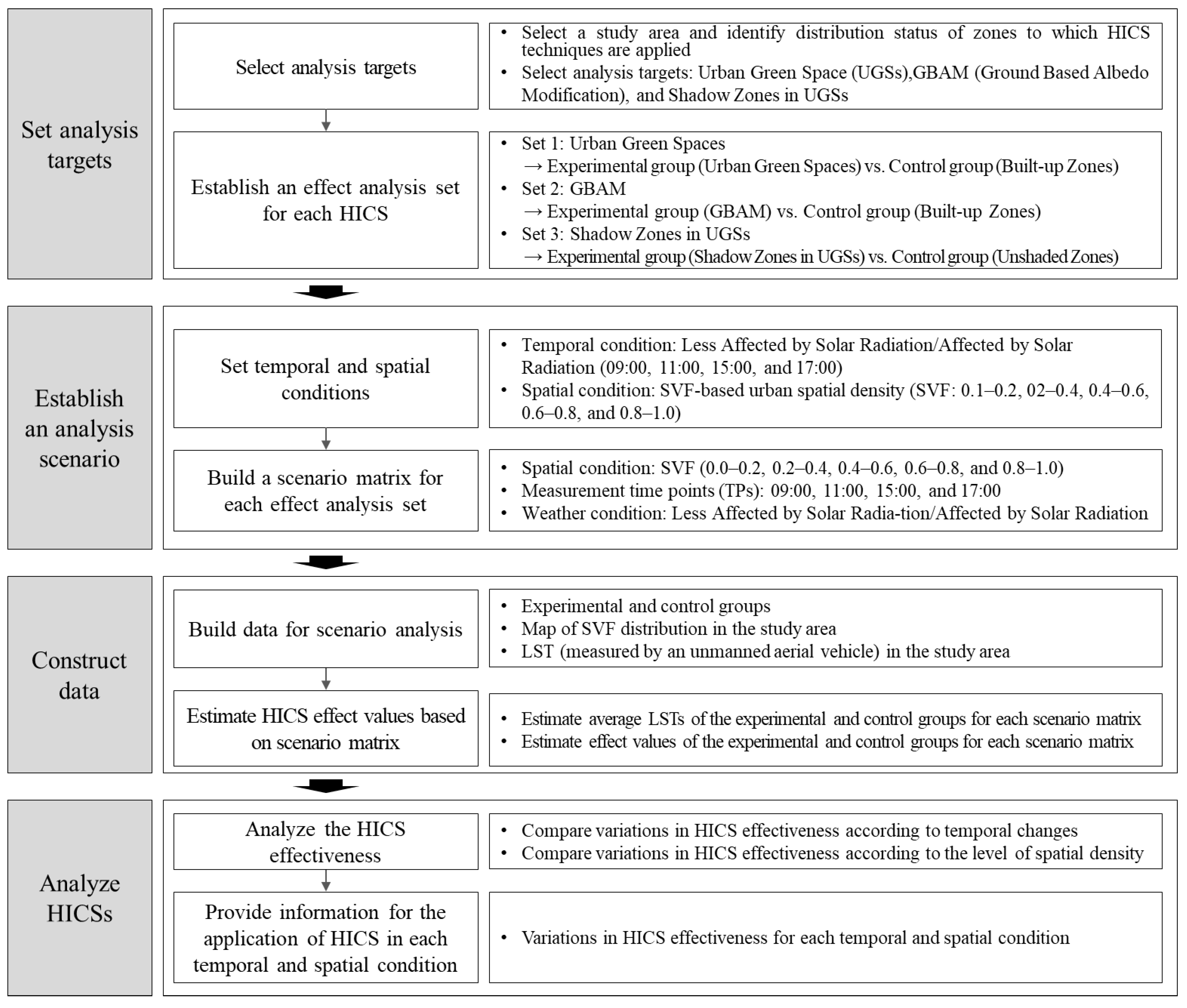
2.1. Methodology
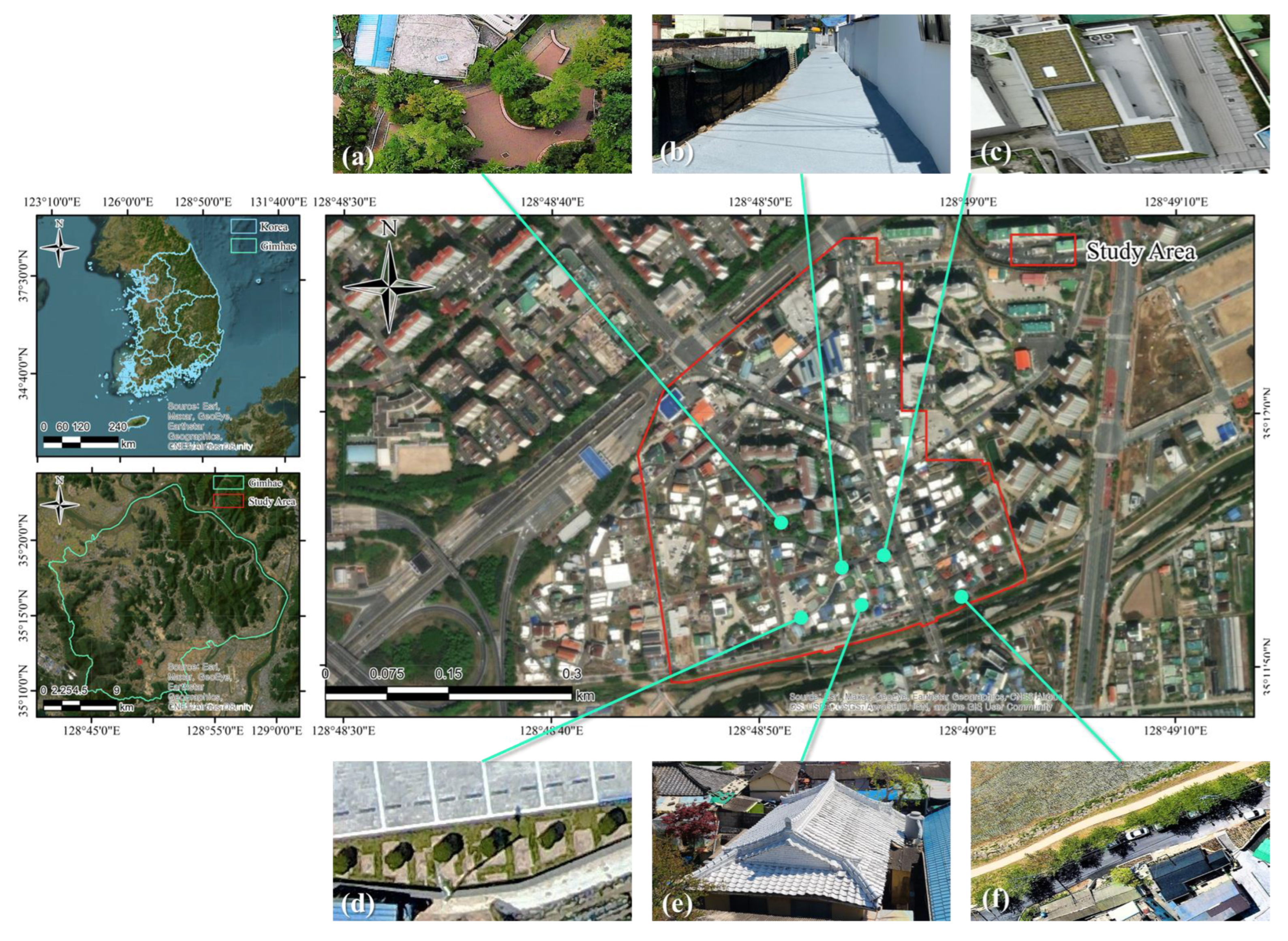
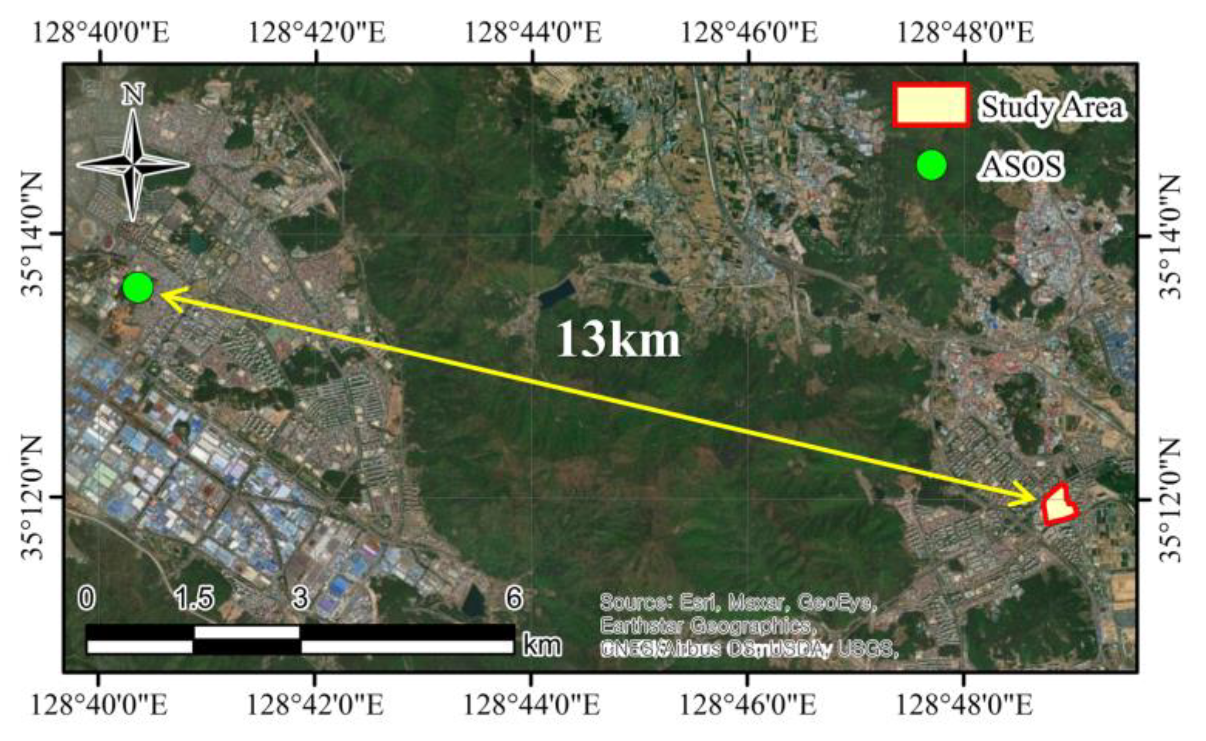
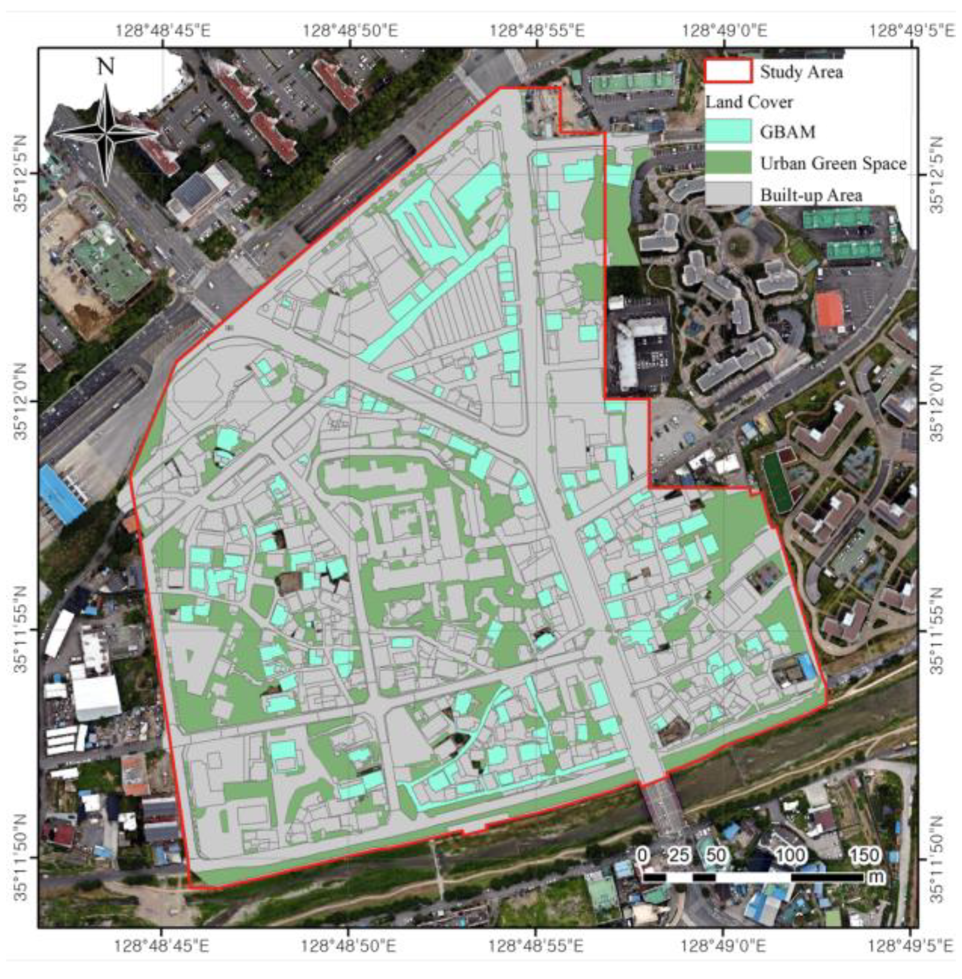
2.1.1. Study Area and Analysis Targets
2.1.2. Scenarios Used to Analyze HICS Effectiveness
2.2. Materials
2.2.1. Areas of Experimental and Control Groups
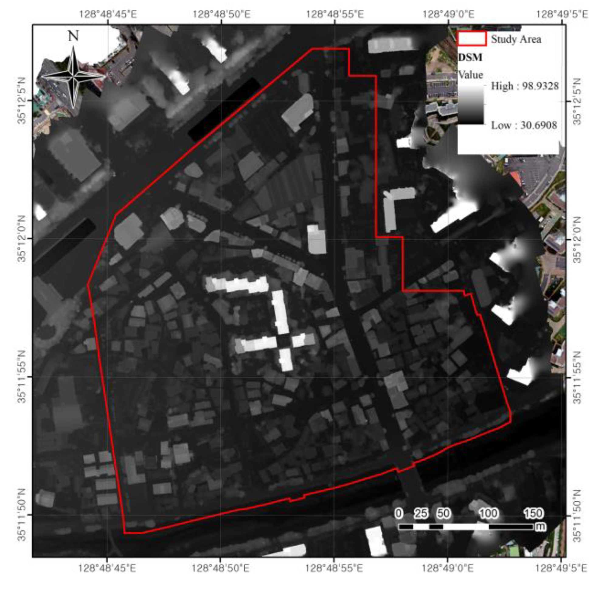
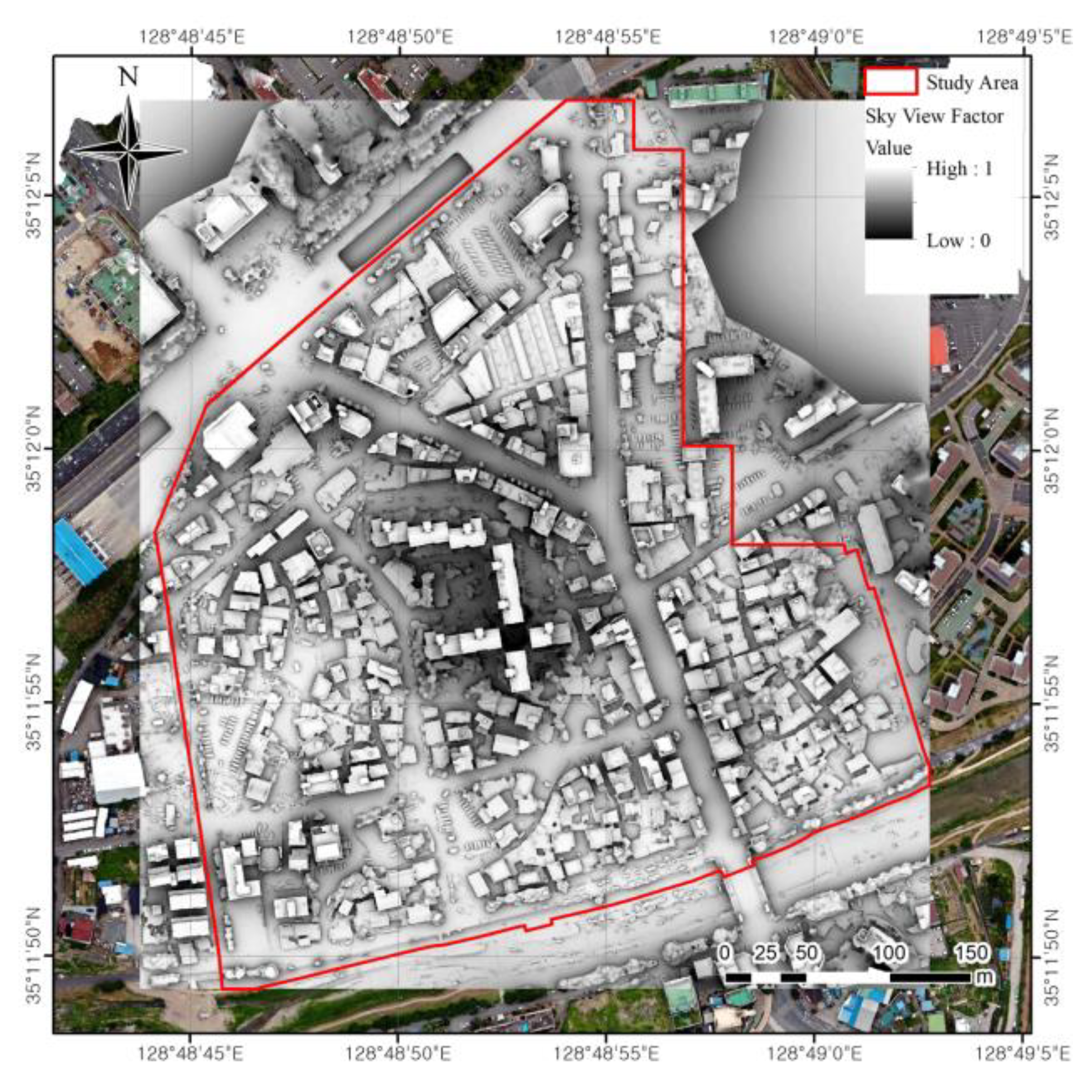
2.2.2. Construction of Urban Morphological Parameters
2.2.3. LST Retrieval
3. Results
3.1. Effectiveness of Urban Green Spaces
3.1.1. Cooling Effects of UGSs for Each Level of SD Based on the Same TP
3.1.2. Range of Variation in Cooling Effects of UGSs for Each Level of SD during the Daytime
3.1.3. Differences in Cooling Effects of UGSs between Morning and Afternoon for Each Level of SD
3.2. Effectiveness of Ground-Based Albedo Modification
3.2.1. Cooling Effects of GBAM for Each Level of SD Based on the Same TP
3.2.2. Range of Variation in Cooling Effects of GBAM for Each Level of SD during the Daytime
3.2.3. Differences in Cooling Effects of GBAM between Morning and Afternoon for Each Level of SD
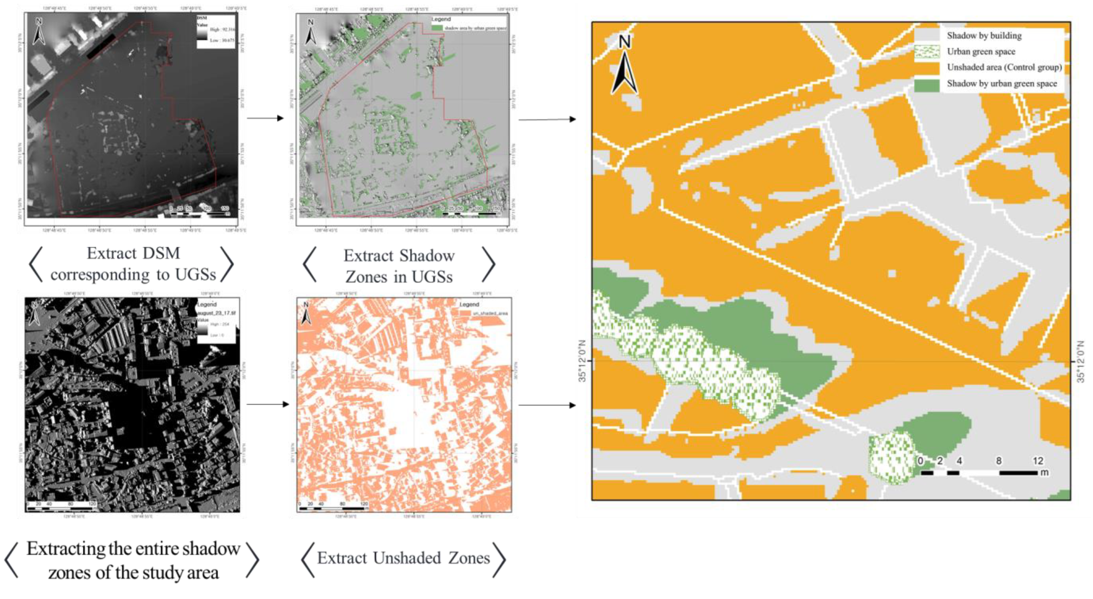
3.3. Effectiveness of Shadow Zones in UGSs
3.3.1. Cooling Effects of Shadow Zones in UGSs for Each Level of SD Based on the Same TP
3.3.2. Range of Variation in Cooling Effects of Shadow Zones in UGSs for Each Level of SD during the Daytime
3.3.3. Differences in Cooling Effects of Shadow Zones in UGSs between Morning and Afternoon for Each Level of SD
4. Discussion
5. Conclusions
5.1. Cooling Characteristics of HICSs
5.2. Implications of This Study
Author Contributions
Funding
Institutional Review Board Statement
Informed Consent Statement
Data Availability Statement
Acknowledgments
Conflicts of Interest
References
- Oke, T.R. The energetic basis of the urban heat island. Q. J. R. Meteorol. Soc. 1982, 108, 1–24. [Google Scholar] [CrossRef]
- Rizvi, S.H.; Alam, K.; Iqbal, M.J. Spatio-temporal variations in urban heat island and its interaction with heat wave. J. Atmos. Sol. Terr. Phys. 2019, 185, 50–57. [Google Scholar] [CrossRef]
- Reducing Urban Heat Islands: Compendium of Strategies; Urban Heat Island Basics. US EPA. 2011. Available online: http://www.epa.gov/heatisland/resources/compendium.htm (accessed on 22 May 2023).
- Yamamoto, Y. Measures to Mitigate Urban Heat Islands; 1349-3663; NISTEP Science & Technology Foresight Center: Tokyo, Japan, 2006. [Google Scholar]
- Ng, E.; Ren, C. The Urban Climatic Map: A Methodology for Sustainable Urban Planning; Routledge: Abingdon, UK, 2015. [Google Scholar]
- World Health Organization; Regional Office for Europe. Urban Green Spaces: A Brief for Action; World Health Organization: Geneva, Switzerland; Regional Office for Europe: Copenhagen, Denmark, 2017. [Google Scholar]
- De Coninck, H.; Revi, A.; Babiker, M.; Bertoldi, P.; Buckeridge, M.; Cartwright, A.; Dong, W.; Ford, J.; Fuss, S.; Hourcade, J.-C. Strengthening and Implementing the Global Response. 2018. Available online: https://www.ipcc.ch/site/assets/uploads/sites/2/2019/02/SR15_Chapter4_Low_Res.pdf (accessed on 22 May 2023).
- Zhao, D.; Aili, A.; Zhai, Y.; Xu, S.; Tan, G.; Yin, X.; Yang, R. Radiative sky cooling: Fundamental principles, materials, and applications. Appl. Phys. Rev. 2019, 6, 021306. [Google Scholar] [CrossRef]
- Konopacki, S.; Gartland, L.; Akbari, H.; Rainer, L. Demonstration of Energy Savings of Cool Roofs; Lawrence Berkeley National Laboratory, Environmental Energy Technologies Division: Berkeley, CA, USA, 1998. [Google Scholar]
- Akbari, H.; Kurn, D.M.; Bretz, S.E.; Hanford, J.W. Peak power and cooling energy savings of shade trees. Energy Build. 1997, 25, 139–148. [Google Scholar] [CrossRef]
- Kurn, D.M.; Bretz, S.E.; Huang, B.; Akbari, H. The Potential for Reducing Urban Air Temperatures and Energy Consumption through Vegetative Cooling; Lawrence Berkeley Laboratory: Berkeley, CA, USA, 1994. [Google Scholar]
- Ko, J.; Schlaerth, H.; Bruce, A.; Sanders, K.; Ban-Weiss, G. Measuring the impacts of a real-world neighborhood-scale cool pavement deployment on albedo and temperatures in Los Angeles. Environ. Res. Lett. 2022, 17, 044027. [Google Scholar] [CrossRef]
- Anting, N.; Din, M.F.M.; Iwao, K.; Ponraj, M.; Siang, A.J.L.M.; Yong, L.Y.; Prasetijo, J. Optimizing of near infrared region reflectance of mix-waste tile aggregate as coating material for cool pavement with surface temperature measurement. Energy Build. 2018, 158, 172–180. [Google Scholar] [CrossRef]
- Sha, A.; Liu, Z.; Tang, K.; Li, P. Solar heating reflective coating layer (SHRCL) to cool the asphalt pavement surface. Constr. Build. Mater. 2017, 139, 355–364. [Google Scholar] [CrossRef]
- Stache, E.; Schilperoort, B.; Ottelé, M.; Jonkers, H.M. Comparative analysis in thermal behaviour of common urban building materials and vegetation and consequences for urban heat island effect. Build. Environ. 2022, 213, 108489. [Google Scholar] [CrossRef]
- Colunga, M.L.; Cambrón-Sandoval, V.H.; Suzán-Azpiri, H.; Guevara-Escobar, A.; Luna-Soria, H. The role of urban vegetation in temperature and heat island effects in Querétaro city, Mexico. Atmósfera 2015, 28, 205–218. [Google Scholar] [CrossRef]
- Ghenai, C.; Rejeb, O.; Sinclair, T.; Almarzouqi, N.; Alhanaee, N.; Rossi, F. Evaluation and thermal performance of cool pavement under desert weather conditions: Surface albedo enhancement and carbon emissions offset. Case Stud. Constr. Mater. 2023, 18, e01940. [Google Scholar] [CrossRef]
- Li, H.; Harvey, J.; Kendall, A. Field measurement of albedo for different land cover materials and effects on thermal performance. Build. Environ. 2013, 59, 536–546. [Google Scholar] [CrossRef]
- Rosso, F.; Pisello, A.L.; Cotana, F.; Ferrero, M. On the thermal and visual pedestrians’ perception about cool natural stones for urban paving: A field survey in summer conditions. Build. Environ. 2016, 107, 198–214. [Google Scholar] [CrossRef]
- Susca, T.; Gaffin, S.R.; Dell’Osso, G.R. Positive effects of vegetation: Urban heat island and green roofs. Environ. Pollut. 2011, 159, 2119–2126. [Google Scholar] [CrossRef] [PubMed]
- Yang, Y.; Xu, Y.; Duan, Y.; Yang, Y.; Zhang, S.; Zhang, Y.; Xie, Y. How can trees protect us from air pollution and urban heat? Associations and pathways at the neighborhood scale. Landsc. Urban Plan. 2023, 236, 104779. [Google Scholar] [CrossRef]
- You, Z.; Zhang, M.; Wang, J.; Pei, W. A black near-infrared reflective coating based on nano-technology. Energy Build. 2019, 205, 109523. [Google Scholar] [CrossRef]
- Hu, D.; Meng, Q.; Schlink, U.; Hertel, D.; Liu, W.; Zhao, M.; Guo, F. How do urban morphological blocks shape spatial patterns of land surface temperature over different seasons? A multifactorial driving analysis of Beijing, China. Int. J. Appl. Earth Obs. Geoinf. 2022, 106, 102648. [Google Scholar] [CrossRef]
- Yin, C.; Yuan, M.; Lu, Y.; Huang, Y.; Liu, Y. Effects of urban form on the urban heat island effect based on spatial regression model. Sci. Total Environ. 2018, 634, 696–704. [Google Scholar] [CrossRef]
- Yu, K.; Chen, Y.; Wang, D.; Chen, Z.; Gong, A.; Li, J. Study of the Seasonal Effect of Building Shadows on Urban Land Surface Temperatures Based on Remote Sensing Data. Remote Sens. 2019, 11, 497. [Google Scholar] [CrossRef]
- Middel, A.; Lukasczyk, J.; Maciejewski, R.; Demuzere, M.; Roth, M. Sky View Factor footprints for urban climate modeling. Urban Clim. 2018, 25, 120–134. [Google Scholar] [CrossRef]
- Oke, T.R. Street design and urban canopy layer climate. Energy Build. 1988, 11, 103–113. [Google Scholar] [CrossRef]
- Scarano, M.; Sobrino, J.A. On the relationship between the sky view factor and the land surface temperature derived by Landsat-8 images in Bari, Italy. Int. J. Remote Sens. 2015, 36, 4820–4835. [Google Scholar] [CrossRef]
- Kim, J.; Lee, D.-K.; Brown, R.D.; Kim, S.; Kim, J.-H.; Sung, S. The effect of extremely low sky view factor on land surface temperatures in urban residential areas. Sustain. Cities Soc. 2022, 80, 103799. [Google Scholar] [CrossRef]
- Wang, K.; Jiang, Q.-G.; Yu, D.-H.; Yang, Q.-L.; Wang, L.; Han, T.-C.; Xu, X.-Y. Detecting daytime and nighttime land surface temperature anomalies using thermal infrared remote sensing in Dandong geothermal prospect. Int. J. Appl. Earth Obs. Geoinf. 2019, 80, 196–205. [Google Scholar] [CrossRef]
- Zheng, Y.; Li, W.; Fang, C.; Feng, B.; Zhong, Q.; Zhang, D. Investigating the Impact of Weather Conditions on Urban Heat Island Development in the Subtropical City of Hong Kong. Atmosphere 2023, 14, 257. [Google Scholar] [CrossRef]
- Jin, M.S. Developing an index to measure urban heat island effect using satellite land skin temperature and land cover observations. J. Clim. 2012, 25, 6193–6201. [Google Scholar] [CrossRef]
- Um, J.-S. Performance evaluation strategy for cool roof based on pixel dependent variable in multiple spatial regressions. Spat. Inf. Res. 2017, 25, 229–238. [Google Scholar] [CrossRef]
- Feng, L.; Tian, H.; Qiao, Z.; Zhao, M.; Liu, Y. Detailed variations in urban surface temperatures exploration based on unmanned aerial vehicle thermography. IEEE J. Sel. Top. Appl. Earth Obs. Remote Sens. 2019, 13, 204–216. [Google Scholar] [CrossRef]
- Naughton, J.; McDonald, W. Evaluating the variability of urban land surface temperatures using drone observations. Remote Sens. 2019, 11, 1722. [Google Scholar] [CrossRef]
- Tepanosyan, G.; Muradyan, V.; Hovsepyan, A.; Pinigin, G.; Medvedev, A.; Asmaryan, S. Studying spatial-temporal changes and relationship of land cover and surface Urban Heat Island derived through remote sensing in Yerevan, Armenia. Build. Environ. 2021, 187, 107390. [Google Scholar] [CrossRef]
- Cho, Y.I.; Yoon, D.; Shin, J.; Lee, M.J. Comparative Analysis of the Effects of Heat Island Reduction Techniques in Urban Heatwave Areas Using Drones. Korean J. Remote Sens. 2021, 37, 1985–1999. [Google Scholar] [CrossRef]
- Matuszko, D. Influence of cloudiness on sunshine duration. Int. J. Climatol. 2012, 32, 1527–1536. [Google Scholar] [CrossRef]
- Cho, Y.I.; Yoon, D.; Lee, M.J. Analysis of Spatial Correlation between Surface Temperature and Absorbed Solar Radiation Using Drone—Focusing on Cool Roof Performance. Korean J. Remote Sens. 2022, 38, 1607–1622. [Google Scholar] [CrossRef]
- Page, J. Chapter II-1-A—The Role of Solar-Radiation Climatology in the Design of Photovoltaic Systems. In McEvoy’s Handbook of Photovoltaics, 3rd ed.; Kalogirou, S.A., Ed.; Academic Press: Cambridge, MA, USA, 2018; pp. 601–670. [Google Scholar]
- Yu, Q.; Ji, W.; Pu, R.; Landry, S.; Acheampong, M.; O’Neil-Dunne, J.; Ren, Z.; Tanim, S.H. A preliminary exploration of the cooling effect of tree shade in urban landscapes. Int. J. Appl. Earth Obs. Geoinf. 2020, 92, 102161. [Google Scholar] [CrossRef]
- ESRI. Hillshade Function. Available online: https://desktop.arcgis.com/en/arcmap/latest/manage-data/raster-and-images/hillshade-function.htm (accessed on 31 May 2023).
- Lindberg, F.; Grimmond, C.S.B. Continuous sky view factor maps from high resolution urban digital elevation models. Clim. Res. 2010, 42, 177–183. [Google Scholar] [CrossRef]
- Maes, W.H.; Steppe, K. Estimating evapotranspiration and drought stress with ground-based thermal remote sensing in agriculture: A review. J. Exp. Bot. 2012, 63, 4671–4712. [Google Scholar] [CrossRef] [PubMed]
- Heinemann, S.; Siegmann, B.; Thonfeld, F.; Muro, J.; Jedmowski, C.; Kemna, A.; Kraska, T.; Muller, O.; Schultz, J.; Udelhoven, T.; et al. Land Surface Temperature Retrieval for Agricultural Areas Using a Novel UAV Platform Equipped with a Thermal Infrared and Multispectral Sensor. Remote Sens. 2020, 12, 1075. [Google Scholar] [CrossRef]
- Aimi, D.; Zimmer, T.; Buligon, L.; de Arruda Souza, V.; Hernandez, R.; Romio, L.; Rubert, G.C.; Diaz, M.B.; Maldaner, S.; Veeck, G.P.; et al. Evaluation of Atmospheric Downward Longwave Radiation in the Brazilian Pampa Region. Atmosphere 2021, 12, 28. [Google Scholar] [CrossRef]
- Watson, I.; Johnson, G. Graphical estimation of sky view-factors in urban environments. J. Climatol. 1987, 7, 193–197. [Google Scholar] [CrossRef]
- Oke, T.R.; Mills, G.; Christen, A.; Voogt, J.A. Urban Climates; Cambridge University Press: Cambridge, UK, 2017. [Google Scholar]
- Xia, Y.; Yabuki, N.; Fukuda, T. Sky view factor estimation from street view images based on semantic segmentation. Urban Clim. 2021, 40, 100999. [Google Scholar] [CrossRef]
- Chen, Q.; Cheng, Q.; Chen, Y.; Li, K.; Wang, D.; Cao, S. The Influence of Sky View Factor on Daytime and Nighttime Urban Land Surface Temperature in Different Spatial-Temporal Scales: A Case Study of Beijing. Remote Sens. 2021, 13, 4117. [Google Scholar] [CrossRef]
- Höppe, P. The physiological equivalent temperature—A universal index for the biometeorological assessment of the thermal environment. Int. J. Biometeorol. 1999, 43, 71–75. [Google Scholar] [CrossRef]
- Simmons, M.T.; Gardiner, B.; Windhager, S.; Tinsley, J. Green roofs are not created equal: The hydrologic and thermal performance of six different extensive green roofs and reflective and non-reflective roofs in a sub-tropical climate. Urban Ecosyst. 2008, 11, 339–348. [Google Scholar] [CrossRef]
- Do Nascimento, A.C.L.; Galvani, E.; Gobo, J.P.A.; Wollmann, C.A. Comparison between Air Temperature and Land Surface Temperature for the City of São Paulo, Brazil. Atmosphere 2022, 13, 491. [Google Scholar] [CrossRef]
- Li, H. Chapter 13—Impacts of Pavement Strategies on Human Thermal Comfort. In Pavement Materials for Heat Island Mitigation; Li, H., Ed.; Butterworth-Heinemann: Boston, MA, USA, 2016; pp. 281–306. [Google Scholar]


| Heat Island Cooling Strategies | Experimental Groups | Control Groups | ||
|---|---|---|---|---|
| Abbreviation | Description | |||
| Vegetation | UGSs [6] | Urban green spaces (UGSs) [6] | Built-up zone | |
| Trees | ||||
| Green roofs | ||||
| Cool pavements | GBAM | Ground-based albedo modification (GBAM) zones [7] | ||
| Cool roofs | ||||
| Shadow of | Vegetation | Shadow zones in UGSs | Shadow zones in urban green spaces | Unshaded zone |
| Tree | ||||
| Green roof | ||||
| HICS | Urban Geography Condition (SVF) | Daytime Condition (Time Points) | Meteorological Condition |
|---|---|---|---|
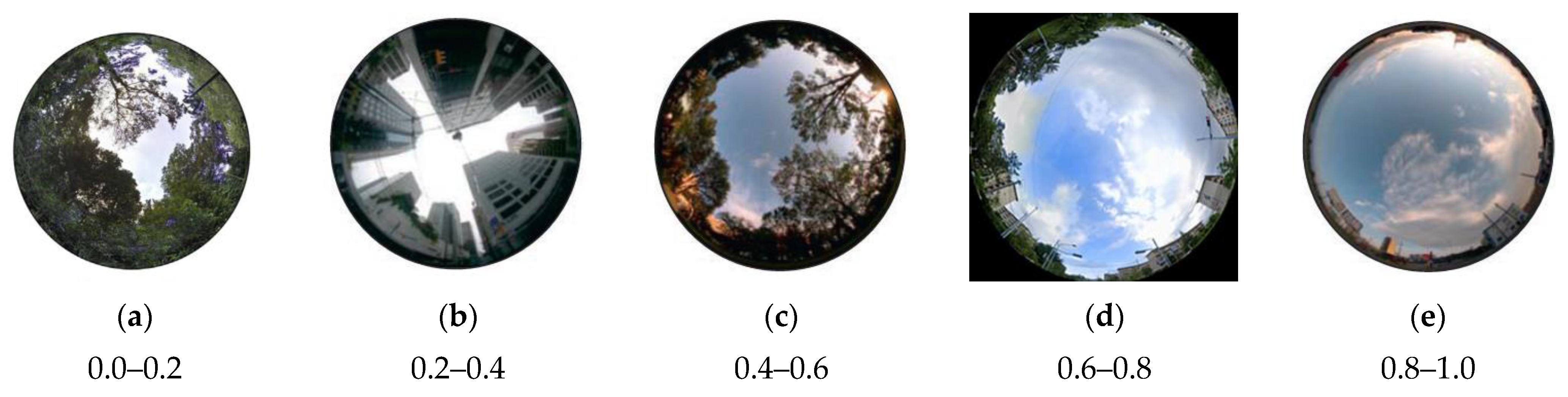
| Urban green spaces (UGSs) | 0.0–0.2 0.2–0.4 0.4–0.6 0.6–0.8 0.8–1.0 | 09:00 11:00 13:00 15:00 17:00 | Less affected by solar radiation |
| Affected by solar radiation | |||
| Ground-based albedo modification (GBAM) zones | 0.0–0.2 0.2–0.4 0.4–0.6 0.6–0.8 0.8–1.0 | 09:00 11:00 13:00 15:00 17:00 | Less affected by solar radiation |
| Affected by solar radiation | |||
| Shadow zones in UGSs | 0.0–0.2 0.2–0.4 0.4–0.6 0.6–0.8 0.8–1.0 | 09:00 11:00 13:00 15:00 17:00 | Less affected by solar radiation |
| Affected by solar radiation |
| Groups | Name | Definition | Data | Type | |
|---|---|---|---|---|---|
| Areas of research targets | Experimental groups | Urban green spaces (UGSs) | Areas covered by vegetation, trees, and green roofs | Land cover map [37] | shp (polygon) |
| Ground-based albedo modification (GBAM) zones | Areas covered by cool pavements and cool roofs | Land cover map [37] | shp (polygon) | ||
| Shadow zones in UGSs * | Areas covered by shadows from vegetation, trees, and green roofs | DSM [39] | tiff (raster) | ||
| Control groups | Built-up zones | Control group for UGSs and GBAM zones | Land cover map [37] | shp (polygon) | |
| Unshaded zones | Control group for shadow zones in UGSs * | DSM [39] | tiff (raster) | ||
| Spatial density (SD) control | Sky view factor (SVF) | Proportion of sky hemisphere visible from the ground | DSM [39] | tiff (raster) | |
| Temperature | Land surface temperature (LST) * | Surface temperature data for study area | Bright temperature, emissivity, Tbkg | tiff (raster) | |
| SVF | 0.0–0.2 | 0.2–0.4 | 0.4–0.6 | 0.6–0.8 | 0.8–1.0 | |
|---|---|---|---|---|---|---|
| Time | ||||||
| Less affected by solar radiation | 9:00 | −0.836 | −1.754 | −2.449 | −2.111 | −4.208 |
| 11:00 | −0.661 | −2.722 | −4.313 | −5.348 | −7.426 | |
| 13:00 | −0.505 | −3.358 | −5.197 | −7.054 | −9.749 | |
| 15:00 | −0.936 | −2.971 | −4.570 | −6.143 | −6.863 | |
| 17:00 | −0.312 | −2.267 | −3.245 | −3.381 | −3.833 | |
| Tmin–Tmax | −0.624 | −1.604 | −2.748 | −4.943 | −5.916 | |
| A.M. | −0.749 | −2.238 | −3.381 | −3.730 | −5.817 | |
| P.M. | −0.624 | −2.619 | −3.908 | −4.762 | −5.348 | |
| TA.M.–TP.M. | −0.125 | 0.381 | 0.527 | 1.033 | −0.469 | |
| Affected by solar radiation | 9:00 | −0.025 | −2.091 | −4.642 | −6.426 | −11.839 |
| 11:00 | −1.208 | −3.819 | −6.757 | −9.018 | −13.704 | |
| 13:00 | −1.678 | −4.730 | −7.510 | −10.015 | −13.328 | |
| 15:00 | −0.775 | −2.856 | −4.938 | −6.743 | −8.224 | |
| 17:00 | −1.072 | −2.444 | −3.938 | −5.050 | −3.887 | |
| Tmin–Tmax | −1.653 | −2.639 | −3.572 | −4.965 | −9.817 | |
| A.M. | −0.617 | −2.955 | −5.700 | −7.722 | −12.772 | |
| P.M. | −0.924 | −2.650 | −4.438 | −5.897 | −6.056 | |
| TA.M.–TP.M. | 0.307 | −0.305 | −1.262 | −1.826 | −6.716 |
| SVF | 0.0–0.2 | 0.2–0.4 | 0.4–0.6 | 0.6–0.8 | 0.8–1.0 | |
|---|---|---|---|---|---|---|
| Time | ||||||
| Less affected by solar radiation | 9:00 | 0.018 | −0.650 | −1.922 | −2.386 | −4.620 |
| 11:00 | 0.701 | −0.250 | −1.918 | −3.379 | −6.494 | |
| 13:00 | 1.025 | −1.102 | −2.750 | −4.277 | −7.900 | |
| 15:00 | 1.167 | 0.452 | −0.930 | −2.966 | −4.263 | |
| 17:00 | 0.971 | −0.246 | −1.704 | −2.110 | −2.803 | |
| Tmin–Tmax | −1.149 | −1.554 | −1.820 | −2.167 | −5.097 | |
| A.M. | 0.360 | −0.450 | −1.920 | −2.883 | −5.557 | |
| P.M. | 1.069 | 0.103 | −1.317 | −2.538 | −3.533 | |
| TA.M.–TP.M. | −0.710 | −0.553 | −0.603 | −0.345 | −2.024 | |
| Affected by solar radiation | 9:00 | 0.842 | 0.180 | −1.605 | −3.101 | −9.462 |
| 11:00 | 0.003 | −0.981 | −3.015 | −4.989 | −10.827 | |
| 13:00 | 0.817 | −0.220 | −2.262 | −5.104 | −9.943 | |
| 15:00 | 0.927 | −0.657 | −2.095 | −2.809 | −5.159 | |
| 17:00 | 0.530 | 0.224 | −0.984 | −2.110 | −1.502 | |
| Tmin–Tmax | −0.924 | −1.205 | −2.031 | −2.994 | −9.325 | |
| A.M. | 0.423 | −0.401 | −2.310 | −4.045 | −10.145 | |
| P.M. | 0.729 | −0.217 | −1.540 | −2.460 | −3.331 | |
| TA.M.–TP.M. | −0.306 | −0.184 | −0.771 | −1.586 | −6.814 |
| SVF | 0.0–0.2 | 0.2–0.4 | 0.4–0.6 | 0.6–0.8 | 0.8–1.0 | |
|---|---|---|---|---|---|---|
| Time | ||||||
| Less affected by solar radiation | 9:00 | −1.104 | −0.865 | 0.206 | −0.042 | −0.467 |
| 11:00 | −0.937 | −0.326 | 0.448 | −0.174 | −2.939 | |
| 13:00 | −0.002 | −0.890 | −0.313 | −0.482 | −2.214 | |
| 15:00 | −0.698 | −0.389 | 0.136 | −0.112 | −1.825 | |
| 17:00 | −0.888 | −0.099 | −0.593 | −0.822 | −0.591 | |
| Tmin–Tmax | −1.102 | −0.791 | −1.041 | −0.780 | −2.472 | |
| A.M. | −1.021 | −0.596 | 0.327 | −0.108 | −1.703 | |
| P.M. | −0.793 | −0.244 | −0.229 | −0.467 | −1.208 | |
| TA.M.–TP.M. | −0.228 | −0.352 | 0.556 | 0.359 | −0.495 | |
| Affected by solar radiation | 9:00 | −2.941 | −3.250 | −2.973 | −2.535 | −5.319 |
| 11:00 | −3.934 | −3.260 | −1.852 | −1.868 | −4.479 | |
| 13:00 | −0.913 | −1.966 | −1.628 | −1.756 | −3.751 | |
| 15:00 | 0.807 | −0.602 | 0.506 | −0.638 | −1.520 | |
| 17:00 | −0.425 | −0.056 | 0.528 | 0.530 | 0.306 | |
| Tmin–Tmax | −4.741 | −3.204 | −3.501 | −3.065 | −5.625 | |
| A.M. | −3.438 | −3.255 | −2.413 | −2.202 | −4.899 | |
| P.M. | 0.191 | −0.329 | 0.517 | −0.054 | −0.607 | |
| TA.M.–TP.M. | −3.629 | −2.926 | −2.930 | −2.148 | −4.292 |
Disclaimer/Publisher’s Note: The statements, opinions and data contained in all publications are solely those of the individual author(s) and contributor(s) and not of MDPI and/or the editor(s). MDPI and/or the editor(s) disclaim responsibility for any injury to people or property resulting from any ideas, methods, instructions or products referred to in the content. |
© 2023 by the authors. Licensee MDPI, Basel, Switzerland. This article is an open access article distributed under the terms and conditions of the Creative Commons Attribution (CC BY) license (https://creativecommons.org/licenses/by/4.0/).
Share and Cite
Cho, Y.-I.; Yoon, D.; Lee, M.-J. Comparative Analysis of Urban Heat Island Cooling Strategies According to Spatial and Temporal Conditions Using Unmanned Aerial Vehicles(UAV) Observation. Appl. Sci. 2023, 13, 10052. https://doi.org/10.3390/app131810052
Cho Y-I, Yoon D, Lee M-J. Comparative Analysis of Urban Heat Island Cooling Strategies According to Spatial and Temporal Conditions Using Unmanned Aerial Vehicles(UAV) Observation. Applied Sciences. 2023; 13(18):10052. https://doi.org/10.3390/app131810052
Chicago/Turabian StyleCho, Young-Il, Donghyeon Yoon, and Moung-Jin Lee. 2023. "Comparative Analysis of Urban Heat Island Cooling Strategies According to Spatial and Temporal Conditions Using Unmanned Aerial Vehicles(UAV) Observation" Applied Sciences 13, no. 18: 10052. https://doi.org/10.3390/app131810052
APA StyleCho, Y.-I., Yoon, D., & Lee, M.-J. (2023). Comparative Analysis of Urban Heat Island Cooling Strategies According to Spatial and Temporal Conditions Using Unmanned Aerial Vehicles(UAV) Observation. Applied Sciences, 13(18), 10052. https://doi.org/10.3390/app131810052