Estimation of Earth’s Central Angle Threshold and Measurement Model Construction Method for Pose and Attitude Solution Based on Aircraft Scene Matching

Abstract

To address the challenge of solving aircraft’s visual navigation results using scene matching, this paper introduces the spherical EPnP positioning posture-solving method, which incorporates the threshold value for the central angle and the construction of a measurement model. The detailed steps are as follows: Firstly, the positioning coordinate model of the Earth’s surface is constructed to ensure the expression of the three-dimensional coordinates of the Earth’s surface. The positioning is then solved by employing the EPnP positioning posture-solving algorithm on the constructed data model. Secondly, by comparing and analyzing the positioning posture values of approximate plane coordinates, the critical value is determined, which serves as a reference for plane calculations. Lastly, a theoretical measurement model for visual height and central angle is constructed, taking into account the decided central angle threshold value. The simulation experiment demonstrates that using spherical coordinates as input results in an average positioning precision that is 16.42 percent higher compared to using plane coordinates as input. When the central angle is less than 0.5 degrees and the surface area is smaller than ${55850}^2$ square meters, the positioning precision of plane coordinates is comparable to that of spherical coordinates. In such instances, the sphere can be approximated as flat. The findings of this study provide important theoretical guidance for further research on scene-matching positioning posture solving. These results hold significant implications for both theoretical research and engineering applications.

1. Introduction

Positioning plays a crucial role in aircraft operations [1,2]. Currently, aircraft navigation systems primarily consist of satellite navigation, satellite-aided inertia combined navigation, and visual navigation [3,4]. Although satellite navigation systems can offer continuous and precise position information, they are susceptible to disruption and deception from anti-satellite devices, leading to incorrect positioning [5,6]. Moreover, the navigation precision of satellite systems deteriorates rapidly when subjected to interference, resulting in errors. In contrast, the performance of an inertia and satellite combined navigation system heavily relies on the precision of the inertial navigation component [7,8]. With high-precision inertial navigation equipment and stable satellite signals, this system facilitates stable aircraft positioning. Visual navigation, on the other hand, boasts low cumulative errors and strong anti-interference capabilities [9,10]. Consequently, visual navigation has found extensive use in terminal guidance applications. To enhance the stability and safety of navigation systems while reducing equipment costs, visual navigation has emerged as the preferred choice [11].

Visual navigation can be broadly categorized into two main types: SLAM (Simultaneous Localization and Mapping), based on image sequences and scene matching, based on a single image [12,13]. In visual SLAM, a visual speedometer can be established by obtaining the successive images’ positioning posture transformation matrix and calculating the corresponding positioning posture information [14]. However, accumulative errors are inherent in this approach, and visual SLAM often requires a large number of distinctive feature points for successful matching, which can be challenging to achieve during high-altitude flights. On the other hand, scene matching offers a reliable alternative for aircraft navigation, as it does not suffer from accumulative errors and exhibits high stability. Scene matching involves determining the absolute positioning information of reference markers on the surface through image matching and subsequently solving for the positioning posture using dedicated algorithms. The precision of scene matching relies not only on the quality of image matching but also on the effectiveness of the algorithm employed.

The PnP (Perspective-n-Point) algorithm is widely recognized as one of the most extensively used algorithms for solving positioning posture due to its excellent stability and efficiency [15,16]. The calculation of PnP attitude relies on a known set of three-dimensional points, which are used to determine their corresponding two-dimensional projection points in the image. This allows for the estimation of the camera’s altitude through the composition of a translation rotation matrix. The translation matrix describes the camera’s position in the world coordinate system, while the rotation matrix characterizes its direction and orientation. Several common PnP algorithms are available, including Perspective-3-Point (P3P) [17], Efficient Perspective-n-Point (EPnP) [18], Direct Linear Transform (DLT) [19], and Uncalibrated Perspective-n-Point (UPnP) [20]. These algorithms are employed in varying situations. Among them, P3P is challenging to utilize in the SLAM algorithm due to difficulties in obtaining an exclusive solution and the requirement for multiple pairs of characteristic points for accurate calculations after optimization. The DLT and UPnP algorithms necessitate at least six pairs of high-quality matching points, making them less suitable for use in multi-modal image matching algorithms involving noisy images. However, EPnP only requires four correctly matched pairs of images to solve the positioning posture and can obtain an exclusive solution. Consequently, it is well-suited for aircraft-based positioning posture solving [21,22].

Image matching of aircraft always uses monocular vision [23,24], which may lead to difficulty in acquiring profound information; consequently, during normal processing, pictures collected are always recognized as planes and the absolute coordinates acquired are always the points within the plane. Additionally, errors may have occurred if we took real-time pictures as a plane to solve the positioning posture. ∆H is the error, shown in the following Figure 1. Because it involves a large number of formulas and coordinate system transformations, the right-handed coordinate system is used in the full text of this article. The whole text $\theta$ represents the angle with the Z-axis, $\phi$ represents the angle with the X-axis, R represents the radius of the Earth, ∆H represents the error, and H is the height of the camera from the ground. In the formula, ‘$\times$’ represents matrix multiplication, whereas ‘$\cdot$’ represents number multiplication.

As is shown in Figure 1, ${\mathrm{O}}_1$ denotes the position of the camera, ${\mathrm{O}}_2$ denotes the center of the Earth, and the surface formed by NM represents the surface of the map that the camera can capture. The camera position ${\mathrm{O}}_1$ is shown to be placed directly above the positive Z-axis for reader comprehension. However, in the actual computational process, the camera position ${\mathrm{O}}_1$ is situated at a general location. The dotted line in the figure is used to make the Earth look more three-dimensional. In the imaging process, since the sphere is approximated as a class plane when the height of the camera increases, an error will generate, which will reduce the accuracy of the positioning attitude solution. Therefore, it is necessary to determine the threshold value of the central angle to estimate the ideal errors of a plane in order to replace the sphere surface and the transmission law. To address this problem, we put forward an approach for a spherical EPnP positioning posture solution by measuring the central angle threshold value for scene matching of aircraft. Based on the above approach, we constructed theoretical models for the flying height and camera field angles, which we named the Earth Model Efficient Perspective-n-Point method (EarM_EPnP). The innovations of the EarM_EPnP method are mainly as follows:

• In this paper, an aircraft positioning posture-solving approach is proposed, utilizing analogous three-dimensional data as input. This method significantly enhances the precision of solving flat coordinates through the application of the EPnP algorithm.
• The replacement of three-dimensional solving in scene matching with a plane ensures the determination of the critical value of the central angle. This theoretical advancement lays the foundation for future investigations into the positioning posture solving of scene matching.
• The parameters of the camera, critical angle, and the inherent relationship among field angles were effectively determined in this study. These findings establish the corresponding functional relationships and provide essential measurement principles for subsequent research in this field.

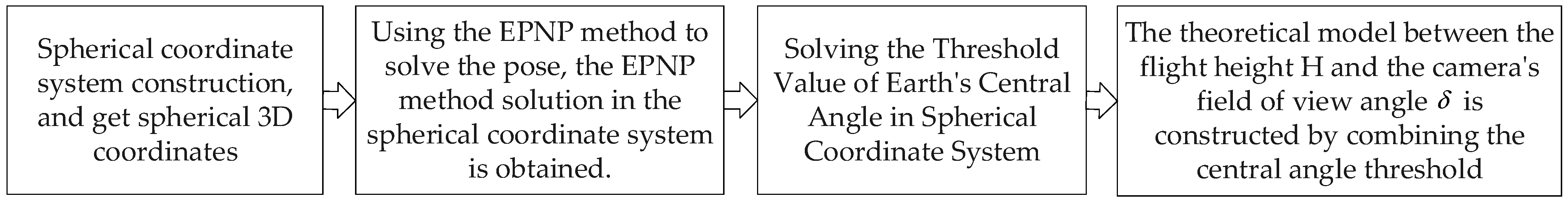
This paper consists of four main sections. The introduction, the first part, provides an overview of the current status of research into solving positioning posture through scene matching. The second part focuses on the unique methodologies employed in this study. Subsequently, the third part presents the experimental findings and corresponding discussions. Finally, the conclusion summarizes the key findings and implications.

2. EarM_EPnP

The flow chart of EarM_EPnP is shown in Figure 2.

The detailed steps of the above picture are described below.

• Setting up the spherical coordinates system and obtaining the spherical coordinates.
• Solving the spherical coordinates based on EPnP and acquiring the results of solving the positioning posture.
• Integrating with the results of EPnP solving and taking GPS precision as a datum to decide the central angle of the Earth.
• Construction of theoretical models for the height of aerial photography, the central angle, and the field angle.

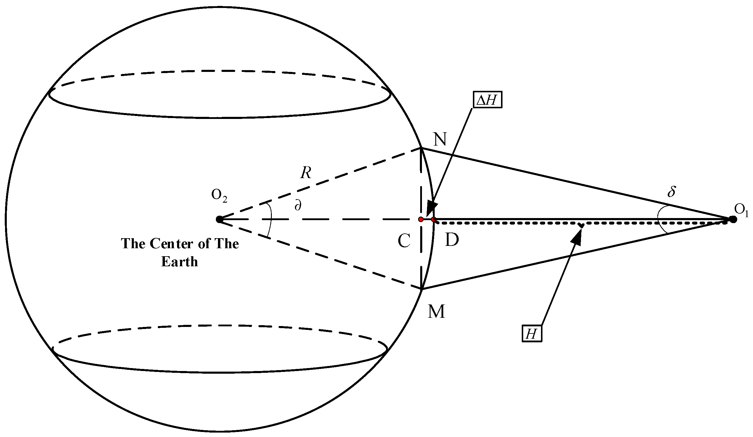
2.1. Construction of Spherical Coordinates

As shown in Figure 1, the downward view is usually used by the aircraft’s monocular vision for data acquisition. For the convenience of calculation, the right-hand coordinate system was established in this paper, and the Z-axis was pointed to the camera by the center of the Earth. For the monocular vision of the aircraft, direct vision and downward vision were used for data acquisition. Since monocular vision could not obtain depth information, the collected datum plane coordinates were approximately three-dimensional coordinates $\left(X,Y,R\right)$ where $R$ denotes the radius of the Earth, and $X,Y$ denote the coordinates on the X-axis and Y-axis. However, the real three-dimensional coordinates of the Earth’s surface should be $\left(X,Y,Z\right)$, where $Z$ represents the coordinates on the Z-axis. If the Earth is regarded as a ball with a radius of $R$, the relationship between the four variables $X,Y,Z,R$ is shown as follows [25].

$$X^2+Y^2+Z^2=R^2$$

(1)

The value of Z in the real coordinate can be obtained by transforming Equation (1) as follows:

$$Z=\sqrt[]{R^2-X^2-Y^2}$$

(2)

According to the expression of the spherical coordinates system, the datum mark coordinates of the Earth’s surface can be written as $\left(X,Y,\sqrt[]{R^2-X^2-Y^2}\right)$. For the convenience of calculating and expressing the relationship of erroneous angles, this paper took polar coordinates, so the spherical coordinates $A^{\prime }$ are:

$$A^{\prime }=\left[\begin{array}{c}X\\ Y\\ Z\end{array}\right]=\left[\begin{array}{l}Rsin\theta cos\phi \\ Rsin\theta sin\phi \\ Rcos\theta \end{array}\right]$$

(3)

As shown in Figure 1, $\theta$ in Equation (3) is the angle with the Z-axis and $\phi$ is the angle with the X-axis. Considering the independence between $\theta$ and $\phi$, we set them at the same angle. Since the settlement point generally requires more than 4, $A^{\prime }$ is a set of points with a number greater than 4. In this paper, ${A^{\prime }}_n$ was used to represent the elements in the solution point set, whose size was a matrix $3\times 1$. The angle $n$ was a natural number, used to represent different points, and n was $\{1,2,3,\dots \}$.

2.2. EPnP Positioning Posture Solving for Spherical Coordinates

In this essay, we used the approaches mentioned in [18] to solve positioning posture. EPnP used the solution point set to calculate the position of the camera in the three-dimensional coordinate system. Since the spherical coordinate system was defined in this method, the position $P_s\left(X_s,Y_s,Z_s\right)$ of the camera in the spherical coordinate system was generated, and the corner $s$ was used to specifically refer to the point that is located in the spherical coordinate system. Similarly, in the altitude calculation process using the classic EPnP, the position $P_f\left(X_f,Y_f,Z_f\right)$ of the camera in the plane coordinate system was generated, and the corner $f$ was used to specifically refer to the point located in the plane coordinate system. The generation process is shown in Equations (4) and (5).

$$\left(R_f,T_f,P_f\right)=f_{EPNP}\left(X_n,Y_n,R\right)$$

(4)

$$\left(R_s,T_s,P_s\right)=f_{EPNP}\left(X_n,Y_n,\sqrt[]{R^2-X_n{}^2-Y_n{}^2}\right)$$

(5)

2.3. Threshold Value of Central Angle

In Section 2.2, this method solved the camera positions in two different coordinate systems. When the height of the camera was low in the sky, the two values $\left(X_s,Y_s,Z_s\right)$ and $\left(X_f,Y_f,Z_f\right)$ were infinitely close, because the radius of the Earth is very large. In the EarM_EPnP method, the circular surface of the sphere is approximated to the plane. However, in the process of increasing the camera height, the error is generated by the traditional EPnP method. As the height increases, the error will continue to increase. The relationship between the camera height and the center angle threshold is better solved, and maximum center angle thresholds with errors within 1 m, 10 m, and 100 m are obtained. In this method, the Earth was regarded as a standard sphere, and the radius was the average radius of the Earth. The EarM_EPnP proposed in this method becomes a true value under this model. $\left(X_s,Y_s,Z_s\right)$ is the real position of the camera under the model. The following is a general formula derivation for calculating the relationship between the height and the central angle within a specific error range.

Firstly, it was necessary to obtain the new coordinates of the solution point set $A^{\prime }$ in the two-dimensional image coordinate system. Through the calculation of Section 2.1 and Section 2.2, the solution point set $A^{\prime }$, the camera’s real position $\left(X_s,Y_s,Z_s\right)$, the EpnP measurement position $\left(X_f,Y_f,Z_f\right)$, and the camera’s internal reference matrix $A$ (the internal reference matrix of each camera is unique) were obtained. The intrinsic matrix A contains the effective focal length values $f_x,f_y$ and the principal point translation values $u_0,v_0$. The internal reference matrix $A$ is shown in Equation (6).

$$A=\left[\begin{array}{ccc}{f}_x& 0& u_0\\ 0& f_y& v_0\\ 0& 0& 1\end{array}\right]$$

(6)

Through the internal parameter matrix $A$, the solution point set $A^{\prime }$ in the spherical coordinate system could be mapped to the two-dimensional image coordinate system. The mapping formula is shown in Equations (7) and (8).

$$X_{{}_{Img\_n}}^S=A\times A_n{}^{\prime }=\left[\begin{array}{l}R\sin \theta \cos \phi \cdot f_x+R\cos \theta \cdot u_0\\ R\sin \theta \sin \phi \cdot f_y+R\cos \theta \cdot v_0\\ R\cos \theta \end{array}\right]$$

(7)

Equation (7) describes the preparation for generating two-dimensional image coordinates by multiplying the coordinates of the Earth’s surface points and the internal reference matrix. In this method, each point in the calculated point set $A^{\prime }$ is brought into Equation (7) for a solution, and a new point set $X_{{}_{Img\_n}}^S$ can be obtained. Each element in the point set is a matrix with a size of $3\times 1$. The number of point sets is also $n$. For subsequent calculations, this method normalizes each element $X_{{}_{Img\_n}}^S$ in the point set $X_{{}_{Img}}^S$, and the normalization method is shown in Equation (8).

$$\left[\begin{array}{ccc}u& v& 1\end{array}\right]=X_{{}_{Img}}^S={\left[\begin{array}{c}\frac{R\sin \theta \cos \phi \cdot f_x+R\cos \theta \cdot u_0}{R\cos \theta }\\ \frac{R\sin \theta \sin \phi \cdot f_y+R\cos \theta \cdot v_0}{R\cos \theta }\\ \begin{array}{c}\\ 1\end{array}\end{array}\right]}^T$$

(8)

In Equation (8), this method divides all the elements $X_{{}_{Img}}^S$ by the third row of elements and then determines the transpose. At this point, the coordinate $A^{\prime }$ of the point set $X_{{}_{3d\_h}}^S$ in the two-dimensional image coordinate system is obtained using Equations (7) and (8).

Secondly, to make the pose of the camera correspond to the position and orientation of the object in the real world, it was necessary to obtain the new coordinates of the solution point set $A^{\prime }$ in the world coordinate system. The origin of the world coordinate system is constantly changing according to the solution point set $A^{\prime }$, and the origin of the world coordinate system can be obtained by calculating the centroid. [18]. The calculation formula of the centroid of the point set $A^{\prime }$ is as follows:

$$\left[\begin{array}{c}{X}_c\\ Y_c\\ Z_c\end{array}\right]=\frac{{\displaystyle \sum _{i=1}^n{A^{\prime }}_i}}{n}$$

(9)

Equation (9) describes the method of obtaining the centroid. Here, $n$ represents the number of point sets, and ${\left[X_c,Y_c,Z_c\right]}^T$ is the position of the origin of the world coordinate system in the three-dimensional Earth coordinate system. At the same time, to make the solution point set $A^{\prime }$ rotate relative to the camera coordinate system, this method uses $\alpha ,\beta ,\gamma$, and $t$ to construct the rotation translation matrix $R_t$. Among them, $\alpha ,\beta ,\gamma$ are the rotation angle on the X-axis, the rotation angle on the Y-axis, and the rotation angle on the Z-axis, and $t$ is the Translation vector. The $t$ is shown in Equation (10).

$$t={\left[\begin{array}{ccc}{t}_x& t_y& t_z\end{array}\right]}^T$$

(10)

The $t$ matrix, $t_x,t_y,t_z$, represents the translation of the X-axis, Y-axis, and Z-axis, respectively. By combining the $\alpha ,\beta ,\gamma$ and $t$ matrices, the rotation translation matrix $R_t$ can be obtained, as shown in Equation (11).

$$R_t=\left[\begin{array}{cccc}\cos (\alpha \left)\cos \right(\gamma )-\cos (\beta \left)\sin \right(\alpha \left)\sin \right(\gamma )& -\cos (\beta \left)\cos \right(\gamma \left)\sin \right(\alpha )-\cos (\alpha \left)\sin \right(\gamma )& \sin (\alpha \left)\sin \right(\beta )& t_x\\ \cos (\gamma \left)\sin \right(\alpha )+\cos (\alpha \left)\cos \right(\beta \left)\sin \right(\gamma )& \cos (\alpha \left)\cos \right(\beta \left)\cos \right(\gamma )-\sin (\alpha \left)\sin \right(\gamma )& -\cos (\alpha \left)\sin \right(\beta )& t_y\\ \sin (\beta \left)\sin \right(\gamma )& \cos (\gamma \left)\sin \right(\beta )& \cos (\beta )& t_z\end{array}\right]$$

(11)

By rotating the translation matrix $R_t$ and ${\left[X_c,Y_c,Z_c\right]}^T$, the new point set $X_{{}_{world\_n}}^S$ in the world coordinate system can be obtained from $A^{\prime }$. The formula for calculating $X_{{}_{world\_n}}^S$ is shown in Equation (12).

$$X_{{}_{world\_n}}^S=R_t\times \left[A_n{}^{\prime }-\left[\begin{array}{c}{X}_c\\ Y_c\\ Z_c\end{array}\right]\right]$$

(12)

Equation (13) bring each point in the solution point set $A^{\prime }$ into the solution, and a new point set $X_{{}_{world\_n}}^S$ can be obtained. Each element in the point set is a matrix $3\times 1$ in size. The number of point sets is also $n$. For subsequent calculations, this method normalized each element $X_{{}_{world}}^S$ in the point set $X_{{}_{world\_n}}^S$, and the normalization processing method was consistent with the processing method of Equation (8). At this point, the coordinate $X_{{}_{3d\_h}}^S$ of the solution point set $A^{\prime }$ in the world coordinate system $R_f$ was obtained.

The coordinates of the solution point set $A^{\prime }$ in the world coordinate system $X_{{}_{3d\_h}}^S$, the coordinates of the solution point set $A^{\prime }$ in the two-dimensional image coordinate system $X_{{}_{3d\_h}}^S$, and the camera’s internal parameter matrix $A$ were calculated again using the method in the paper [18]. The rotation matrix $R_f$, the translation vector $T_f$, and the position coordinates of the camera $P_f$ are as shown in Equation (13).

$$\left(R_f,T_f,P_f\right)=f_{EPnP}\left(X_{{}_{3d\_h}}^S,X_{{}_{2d\_h}}^S,A\right)$$

(13)

To obtain the rotation matrix $R_f$ and the translation vector $T_f$, it is only required to define the initial position $P_0\left[\begin{array}{ccc}0& 0& 0\end{array}\right]$ of the camera. The relative position of the camera in the spherical model can be obtained using Equations (14) and (15).

$$P_s=R_S\times P_0^T+T_S$$

(14)

$$P_f=R_f\times P_0^T+T_f$$

(15)

We identified the difference between the positions acquired by the two formulas above and then took the absolute value to obtain the positioning error.

$$P_{error}=abs(P_f-P_s)$$

(16)

$P_{error}$ represents the positioning solving errors of the plane coordinates system, and $P_s$ and $P_f$, respectively, describe the positioning solving results from the spherical and plane coordinate systems. When $P_{error}$ was 1 m, 10 m, or 100 m, the central angle was the threshold value.

2.4. Model of Aerial and Field of View Angle under Fixed Central Angle

In Section 2.3, using EPnP, we solved the threshold value of the central angle, thereby calculating the theoretical model for the height of aerial photography and field angle. It is shown in the following picture.

It can be seen from Figure 3 that ${\mathrm{O}}_1$ and ${\mathrm{O}}_2$ are the camera and the Earth’s center, respectively. AB represents the arc of the Earth’s surface. C is the center of the plane, and D is the center of the arc of the Earth’s surface. These two points are located at the intersection of the ${\mathrm{O}}_1$ and ${\mathrm{O}}_2$ lines. The central angle is denoted as “$\partial$” and the camera field of view angle is denoted as “$\delta$”.

$$W=2R\sin \left(\partial /2\right)$$

(17)

$W$ represents the length of the line segment $\left|AB\right|$, R represents the radius of the Earth, and $\partial$ is the central angle of the Earth. Additionally, the flying height of the aircraft is $H$.

$$H=H_1-\Delta H$$

(18)

$H$ is the flying height and $H_1$ is the length of $\left|C{O}_1\right|$, in other words, the height errors plus flying height. $\Delta H$ is the length of the segment $\left|CD\right|$, so the height error is:

$$\Delta H=R-R\cos \left(\frac{\partial }{2}\right)$$

(19)

And:

$$H_1=\frac{W}{2\tan \left(\delta /2\right)}$$

(20)

$H_1$ is the length of the segment $\left|C{O}_1\right|$ in other words, the flying height plus the height errors. So, the function for flying height H and field angle $\delta$ is as follows. Equation (21) describes the relationship between $\delta$ and $H$. Equation (22) is used to represent the relationship between $H$ and $\delta$.

$$H=R\cdot \sin \left(\partial /2\right)÷\tan \left(\delta /2\right)-R+R\cos \left(\partial /2\right)$$

(21)

$$\delta =2\arctan \left[R\cdot \sin \left(\frac{\partial }{2}\right)\cdot {\left(H+R-R\cdot \cos \left(\frac{\partial }{2}\right)\right)}^{-1}\right]$$

(22)

3. Simulative Experiment and Discussion

3.1. Experimental Conditions

The experimental platform used was an X64 embedded device based on a 64-bit Windows 10 operating system and an Intel Core i7-7500U CPU processor with a main frequency of 4 GHz. Based on the code in reference [11] and the spherical coordinates in Section 2.1, this method implemented the EarM_EPnP code and EPnP code on Matlab 2018. In this chapter, all the method comparisons were implemented on Matlab 2018.

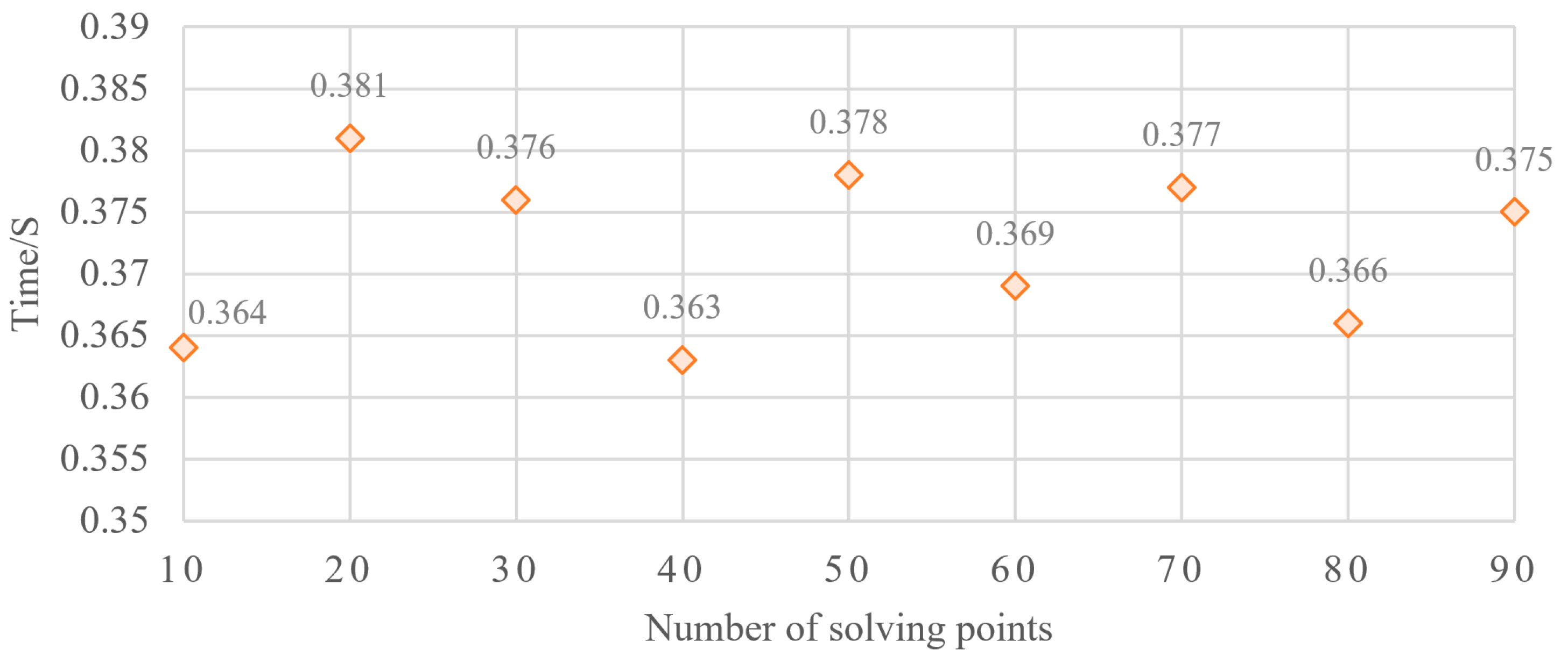
3.2. Ablation Experiments of EarM_EPnP in Different Solution Points

Considering the relationship between the number of solution points and the average error, and the relationship between the number of solution points and the calculation time in the calculation process of the EarM_EPNP algorithm, we design different numbers of solution points to calculate the average error and calculation time. In this experiment, spherical coordinates were used as data markers to record the average error and calculation time. The experimental results are shown in Figure 3 and Figure 4.

It can be seen from Figure 4 and Figure 5. that there was no obvious relationship between the solution time and the number of solution points, and it did not continue to increase with the increase of the number of solution points. At the same time, there was no obvious relationship between the average error corresponding to different solution points. Therefore, we used the actual simulation as the benchmark to use the solution point number of 30.

3.3. Errors of EPnP under Different Central Angle Thresholds

When the maximum threshold of the Earth’s central angle is 0.6 degrees, the average radius of the Earth, $R=6400 \mathrm{km}$. The diameter range of the largest surface circular area that the central angle can cover is $R\times \sin \left(0.6\right)$, about $67.02 \mathrm{km}$. Figure 6 shows that when the number of calculation points is 30 and the flight height is 30 km, the error of the EPnP algorithm under the EarM_EPnP model can be obtained by changing the size of the central angle.

As shown in Figure 6, the central angle also ranges from 0 to 0.6 degrees. The upper-left figure shows the results of X, Y, and Z orientation. From the figure, it can be understood that when the central angle is relatively small (about 0.5 degrees), the results obtained from both the planar solution and the spherical solution are nearly identical, with an error of approximately the GPS error (about 10 m). When the central angle is 0.18 degrees, the error is approximately 1 m. However, as the central angle becomes bigger, errors become bigger, too. If analyzing the X, Y, and Z orientation separately, the errors of direction X and Y become bigger as the central angle increase. Additionally, the fluctuation in direction Z is relatively dramatic.

To further demonstrate the improved accuracy of EarM_EPnP compared to the EPnP method, this paper defines the formula for calculating the positioning accuracy, denoted as ‘$\eta$’:

$$\eta =\left|\frac{p_s-p_f}{p_s}\right|$$

(23)

As the central angle continuously varies from 0 degrees to 0.6 degrees, according to Equation (23), the average positioning accuracy is determined to be 16.42%. When central angle $\partial =0.5$, and the average radius of earth $R=6400 \mathrm{km}$, the maximum surface area covered by central angle can be calculated $6400 \mathrm{km}$ this method by using $R\times \sin (\partial )$. By the way, the maximum length of a side in this surface is about $55850 \mathrm{m}$. If the surface is seen as a square, its area is ${55850}^2$ square meters.

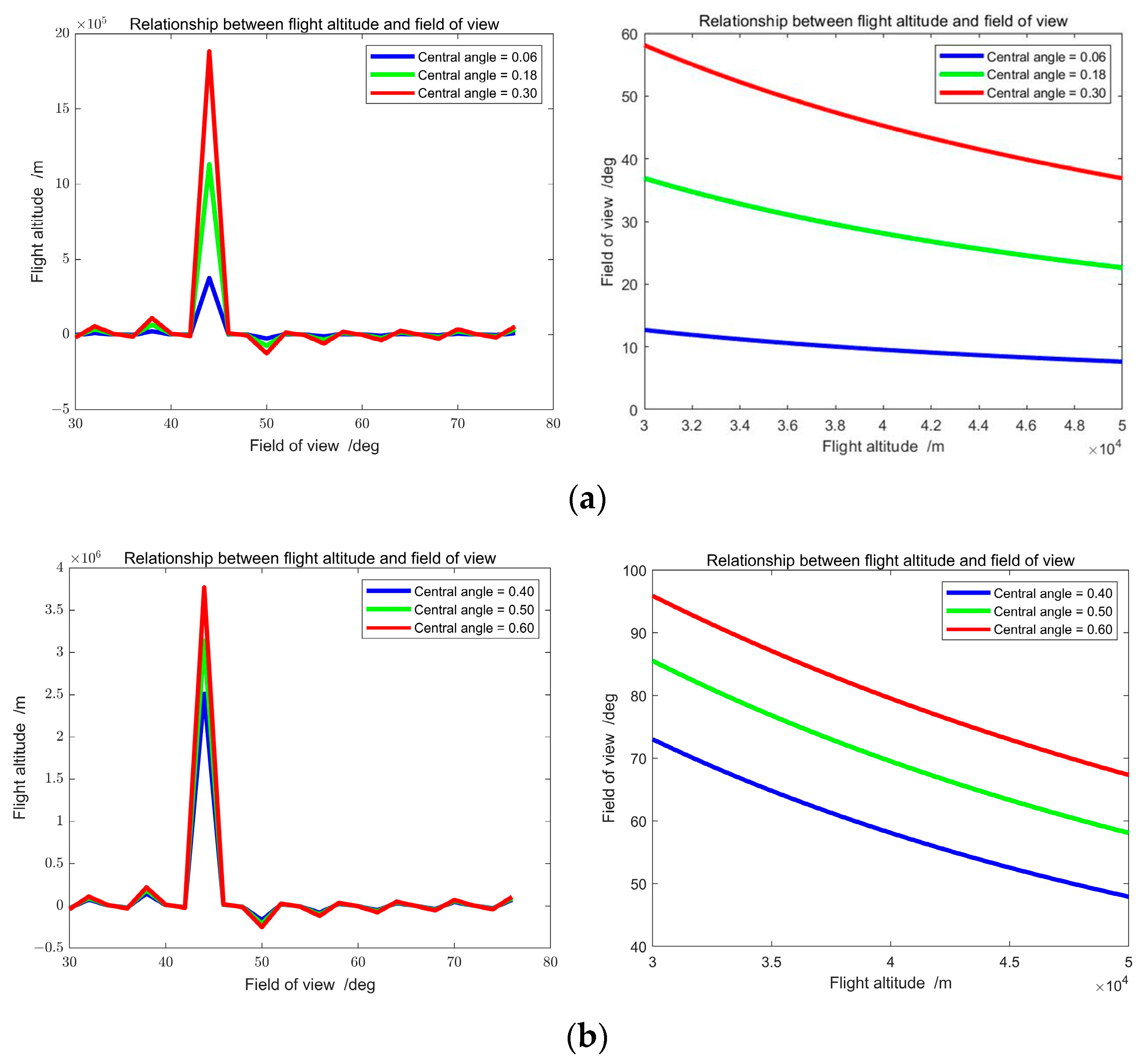
3.4. The Relationship between Flight Height and Field Angle

Before calculating the relationship between the attitude error and the maximum central angle, we needed to select the appropriate camera to obtain the field angle range required for the experiment. We selected the camera field of view range when the central angles were 0.06 degrees, 0.18 degrees, 0.3 degrees, 0.5 degrees, and 0.6 degrees, with a flight height ranging from 30 $\mathrm{km}$ to 50 $\mathrm{km}$. The experimental results are shown in Figure 7.

Figure 7a illustrates the relationship between the field of view angle and flight height for three central angles: 0.06, 0.18, and 0.30 degrees. Flight height and field of view angle can be deduced from each other. With knowledge of the field of view angle, the corresponding flight height can be inferred. Conversely, when the height is known, the corresponding field of view angle can be determined. Similarly, Figure 7b depicts the relationship between the field of view angle and flight height for three central angles: 0.4, 0.5, and 0.6 degrees.

3.5. Experiment on the Relationship between Attitude Error and Maximum Central Angle

Based on the experiments in Section 3.1 and Section 3.2, the EPnP algorithm will have a huge error in the EarM_EPnP model due to the increase of the central angle, and it was verified that the number of solution points of the EPnP algorithm in the EarM_EPnP model is not related to the accuracy. Based on the above experiments, we calculated the maximum center angle that can be obtained when the positioning error is less than 1 m when the positioning error is less than 10 m, and when the positioning error is less than 100 m. The experimental results are shown in Figure 8.

Figure 8 illustrates that at a flight height of 40 km, the field angle varies with the central angle and consistently focuses on the Earth’s surface. In the scatter plot, the horizontal axis represents angles in radians, and the vertical axis represents errors in meters. We calculated the error of the EPnP method on the X-axis by manipulating the central angle. The errors within the ranges of 0–1 m, 1–10 m, and 10–100 m were recorded. Figure 8a depicts the central angle range for errors between 0–1 m. When the error is 1 m, this method yields a critical value of 0.057 degrees for the central angle. Figure 8b presents the central angle range for errors between 1–10 m. With a 10 m error, the critical value of the central angle obtained by this method is 0.179 degrees. Figure 8c showcases the central angle range for errors between 10–100 m. Notably, when the error reaches 100 m, significant oscillations are observed. Additionally, for each case, this paper provides the corresponding mean and variance within the specified range.

3.6. Discussion

This paper investigates the transformation of coordinates from plane coordinates to spherical coordinates. The accuracy of positioning was enhanced in the x and y directions, while some fluctuations were observed in the z-direction. The inclusion of an altimeter in the navigation system can effectively measure altitude, thereby complementing the entire navigation process. Furthermore, the experimental results establish a relationship between flight height and the field of view of the visual sensor at a specific central angle of the Earth. These findings offer valuable theoretical support for the autonomous flight of future aircraft. The specific discussions are as follows:

• This spherical model is a more realistic representation of the Earth and using the spherical model in the PNP (Perspective-n-Point) method provides more accurate positioning information for the aircraft. However, the spherical model is complex and challenging to use in practical applications due to sensor limitations. This paper derives the error propagation relationship of the spherical model and calculates corresponding central angle thresholds for errors of 1 m, 10 m, and 100 m. This simplifies the approach for engineering applications.
• The paper presents the functional relationship between flight altitude and camera field of view. By considering different error ranges, the sensor field of view can be determined in conjunction with the flight altitude. Conversely, based on the given sensor field of view and error requirements, the accurate flight altitude can be determined, providing convenience for practical applications.
• The experimental results demonstrate that the central angle threshold can be accurately and stably determined on the X and Y axes. However, there is fluctuation and simplicity on the Z-axis, indicating a limitation. Engineering applications can utilize complementary sensors such as altimeters to address this issue and it also serves as a key aspect for further research.

4. Conclusions

To address the challenges associated with solving the positioning posture of aircraft scene matching, this paper proposes a method that utilizes three-dimensional coordinates. The experimental results demonstrate that employing high-precision three-dimensional calculations improves the overall precision by 16 percent, offering effective solutions for solving the positioning posture in visual navigation. Additionally, this study accurately deduced the theoretical models and conducted analytical research on the relationship between flying height and field angle. The findings not only provide theoretical guidance for further research on improving flying height and orbit in aircraft scene matching but also hold significant implications for both theoretical investigation and practical applications. However, it is important to note that in the next phase of this research, the focus will shift toward the theoretical analysis of the tendencies of errors corresponding to different angle ranges.

References

1. Hadfield, S.; Lebeda, K.; Bowden, R. HARD-PnP: PnP Optimization Using a Hybrid Approximate Representation. IEEE Trans. Pattern Anal. Mach. Intell. 2019, 41, 768–774. [Google Scholar] [CrossRef] [PubMed]
2. Xu, C.; Zhang, L.; Cheng, L.; Koch, R. Pose Estimation from Line Correspondences: A Complete Analysis and a Series of Solutions. IEEE Trans. Pattern Anal. Mach. Intell. 2017, 39, 1209–1222. [Google Scholar] [CrossRef] [PubMed]
3. Zhou, H.; Zhang, T.; Jagadeesan, J. Re-weighting and 1-Point RANSAC-Based PnP Solution to Handle Outliers. IEEE Trans. Pattern Anal. Mach. Intell. 2019, 41, 1209–1222. [Google Scholar] [CrossRef]
4. Chen, B.; Parra, Á.; Cao, J.; Li, N.; Chin, T.J. End-to-End Learnable Geometric Vision by Backpropagating PnP Optimization. In Proceedings of the 2020 IEEE/CVF Conference on Computer Vision and Pattern Recognition (CVPR), Seattle, WA, USA, 14–19 June 2020; pp. 124–127. [Google Scholar]
5. Qiu, J.; Wang, X.; Fua, P.; Tao, D. Matching Seqlets: An Unsupervised Approach for Locality Preserving Sequence Matching. IEEE Trans. Pattern Anal. Mach. Intell. 2021, 43, 745–752. [Google Scholar] [CrossRef] [PubMed]
6. Bekkers, E.J.; Loog, M.; ter Haar Romeny, B.M.; Duits, R. Template Matching via Densities on the Roto-Translation Group. IEEE Trans. Pattern Anal. Mach. Intell. 2018, 40, 452–466. [Google Scholar] [CrossRef]
7. He, Z.; Jiang, Z.; Zhao, X.; Wu, C. Sparse Template-Based 6-D Pose Estimation of Metal Parts Using a Monocular Camera. IEEE Trans. Ind. Electron. 2020, 67, 390–401. [Google Scholar] [CrossRef]
8. An, Y.; Wang, L.; Ma, R.; Wang, J. Geometric Properties Estimation from Line Point Clouds Using Gaussian-Weighted Discrete Derivatives. IEEE Trans. Ind. Electron. 2021, 68, 703–714. [Google Scholar] [CrossRef]
9. Yu, J.; Hong, C.; Rui, Y.; Tao, D. Multitask Autoencoder Model for Recovering Human Poses. IEEE Trans. Ind. Electron. 2018, 65, 5060–5068. [Google Scholar] [CrossRef]
10. Zhang, J.; Liu, Z.; Gao, Y.; Tao, D. Robust Method for Measuring the Position and Orientation of Drogue Based on Stereo Vision. IEEE Trans. Ind. Electron. 2021, 68, 4298–4308. [Google Scholar] [CrossRef]
11. Lee, T.-J.; Kim, C.-H.; Cho, D.-I.D. A Monocular Vision Sensor-Based Efficient SLAM Method for Indoor Service Robots. IEEE Trans. Ind. Electron. 2019, 66, 318–328. [Google Scholar] [CrossRef]
12. Sun, Y.; Chen, J.; Yuen, C.; Rahardja, S. Indoor Sound Source Localization With Probabilistic Neural Network. IEEE Trans. Ind. Electron. 2018, 65, 6403–6413. [Google Scholar] [CrossRef]
13. Wu, J.; She, J.; Wang, Y.; Su, C.Y. Position and Posture Control of Planar Four-Link Underactuated Manipulator Based on Neural Network Model. IEEE Trans. Ind. Electron. 2020, 67, 4721–4728. [Google Scholar] [CrossRef]
14. Seadawy, A.R.; Rizvi, S.T.R.; Ahmad, S.; Younis, M.; Baleanu, D. Lump, lump-one stripe, multiwave and breather solutions for the Hunter–Saxton equation. Open Phys. 2021, 19, 1–10. [Google Scholar] [CrossRef]
15. Ahmad, H.; Seadawy, A.R.; Khan, T.A. Numerical solution of Korteweg–de Vries-Burgers equation by the modified variational iteration algorithm-II arising in shallow water waves. Phys. Scr. 2020, 95, 045210. [Google Scholar] [CrossRef]
16. Seadawy, A.R.; Kumar, D.; Chakrabarty, A.K. Dispersive optical soliton solutions for the hyperbolic and cubic-quintic nonlinear Schrödinger equations via the extended sinh-Gordon equation expansion method. Eur. Phys. J. Plus 2018, 133, 182. [Google Scholar] [CrossRef]
17. Cranor, L.F. P3P: Making privacy policies more useful. IEEE Secur. Priv. 2003, 1, 50–55. [Google Scholar] [CrossRef]
18. Lepetit, V.; Moreno-Noguer, F.; Fua, P. EP n P: An accurate O (n) solution to the P n P problem. Int. J. Comput. Vis. 2009, 81, 155–166. [Google Scholar] [CrossRef]
19. Shapiro, R. Direct linear transformation method for three-dimensional cinematography. Research Quarterly. Am. Alliance Health Phys. Educ. Recreat. 1978, 49, 197–205. [Google Scholar] [CrossRef]
20. Penate-Sanchez, A.; Andrade-Cetto, J.; Moreno-Noguer, F. Exhaustive linearization for robust camera pose and focal length estimation. IEEE Trans. Pattern Anal. Mach. Intell. 2013, 35, 2387–2400. [Google Scholar] [CrossRef]
21. Younas, U.; Seadawy, A.R.; Younis, M.; Rizvi, S.T.R. Optical solitons and closed form solutions to the (3 + 1)-dimensional resonant Schrödinger dynamical wave equation. Int. J. Mod. Phys. B 2020, 34, 2050291. [Google Scholar] [CrossRef]
22. Seadawy, A.R.; Cheemaa, N. Some new families of spiky solitary waves of one-dimensional higher-order K-dV equation with power law nonlinearity in plasma physics. Indian J. Phys. 2020, 94, 117–126. [Google Scholar] [CrossRef]
23. Wang, C.; Wang, Y.; Lin, Z.; Yuille, A.L. Robust 3D Human Pose Estimation from Single Images or Video Sequences. IEEE Trans. Pattern Anal. Mach. Intell. 2019, 41, 1227–1241. [Google Scholar] [CrossRef] [PubMed]
24. Lee, Y.; Kyung, C.-M. A Memory- and Accuracy-Aware Gaussian Parameter-Based Stereo Matching Using Confidence Measure. IEEE Trans. Pattern Anal. Mach. Intell. 2021, 43, 1845–1858. [Google Scholar] [CrossRef] [PubMed]
25. Schetselaar, E.M. Fusion by the IHS transform: Should we use cylindrical or spherical coordinates? Int. J. Remote Sens. 1998, 19, 759–765. [Google Scholar] [CrossRef]
Figure 1. PNP surface error model.
Applsci 13 10051 g001
Figure 2. Flow chart of EarM_EPnP.
Applsci 13 10051 g002
Figure 3. The relationship between flying height and field angle.
Applsci 13 10051 g003
Figure 4. The relationship between the number of calculation points and the average error.
Applsci 13 10051 g004
Figure 5. The relationship between the number of calculation points and the calculation time.
Applsci 13 10051 g005
Figure 6. Relationship between central angle and the positioning error.
Applsci 13 10051 g006
Figure 7. Relationship between flying height and field angle. (a) Relationship between flight height and field of view angle when the error is 1 m. (b) Relationship between flight height and field of view angle when the error is 10 m.
Applsci 13 10051 g007
Figure 8. Angles, errors, average errors, and variance diagram for the precisions of 1 m, 10 m and 100 m. (a) Precision of 1 m. (b) Precision of 10 m. (c) Precision of 100 m.
Applsci 13 10051 g008
Disclaimer/Publisher’s Note: The statements, opinions and data contained in all publications are solely those of the individual author(s) and contributor(s) and not of MDPI and/or the editor(s). MDPI and/or the editor(s) disclaim responsibility for any injury to people or property resulting from any ideas, methods, instructions or products referred to in the content.