Event-Sampled Adaptive Neural Course Keeping Control for USVs Using Intermittent Course Data

Abstract

This paper addresses the issue of course keeping control (CKC) for unmanned surface vehicles (USVs) under network environments, where various challenges, such as network resource constraints and discontinuities of course and yaw caused by data transmission, are taken into account. To tackle the issue of network resource constraints, an event-sampled scheme is developed to obtain the course data, and a novel event-sampled adaptive neural-network-based state observer (NN–SO) is developed to achieve the state reconstruction of discontinuous yaw. Using a backstepping design method, an event-sampled mechanism, and an adaptive NN–SO, an adaptive neural output feedback (ANOF) control law is designed, where the dynamic surface control technique is introduced to solve the design issue caused by the intermission course data. Moreover, an event-triggered mechanism (ETM) is established in a controller–actuator (C–A) channel and a dual-channel event-triggered adaptive neural output feedback control (ETANOFC) solution is proposed. The theoretical results show that all signals in the closed-loop control system (CLCS) are bounded. The effectiveness is verified through numerical simulations.

1. Introduction

USVs are highly regarded in the field of ocean engineering and have attracted attention from various disciplines, including control systems and ship engineering [1,2,3,4]. In practice, the practical tasks of USVs include path following, tracking control, stability control, dynamic positioning, and CKC [5,6]. For these control tasks, the issue of CKC is one of the most common control problems, which is to make USVs sail along a given trajectory by controlling the steering equipment [7,8,9].

For the issue of CKC, many effective design approaches have been reported, such as active disturbance rejection control (ADRC) [10], PID [11], backstepping [12], sliding mode control (SMC) [13], and H∞ [14]. Furthermore, intelligent ADRC [15], fuzzy PID [16,17], neural PID [18], adaptive backstepping [19], and non-fragile H∞ [20] are proposed to resolve the issue of CKC for USVs. Under these control schemes, the desired control performance was obtained. However, these control schemes are based on the assumption that the course and yaw must be continuously available. Unfortunately, the navigation control of USVs is carried out under a network environment, which implies that the continuous signals required by the navigation control cannot be obtained. For such a case, under a network environment, the superior control schemes mentioned above cannot be transplanted to resolve such CKC design issues of USVs since the signals cannot be guaranteed to be transmitted continuously.

Under a network environment, the CKC system of USVs is a typical cyber-physical system. In this case, several challenging problems should be taken into account in the control design, for example, the network resource constraint problem caused by the network bandwidth, the discontinuity of course and yaw caused by the data transmission process, and so on. In the existing works, event-triggering control (ETC) [21,22] can reduce the data transmission such that the constrained issue of network resource can be relaxed. Unlike the traditional time-triggered control methods, in the ETC-based method, an ETM is constructed in the controller–actuator (C–A) channel. Thus, the control commands are transmitted as long as the preset triggering condition is satisfied. In this context, several ETC-based schemes were reported for the control issue of USVs, like course tracking control [23], tracking control [24,25], and stable control [26]. However, the event-triggering mechanism (ETM) in references [23,24,25,26] is only established between the controller and the actuator, which implies that the transmission of course data cannot be resolved. To further save the network resources, it is essential that a minimum amount of data is transmitted, i.e., in reducing the transmission of control commands and course data at the same time. Obviously, there is a need to explore a new method to solve the problem of limited network resources.

Based on the above observation, this work discusses an event-sampled adaptive neural CKC problem for USVs. An ETM is established in the sensor–controller (S–C) channel, and an event-sampled mechanism (ESM) is developed to obtain the course data, such that only the intermittent course data are transmitted in the control design. To resolve the control design issue caused by the absence of yaw, a novel event-sampled adaptive NN–SO is developed to achieve the refactoring of yaw. In addition, to save the network resource, a ETM is established in the controller–actuator (C–A) channel. Finally, a dual-channel ETANOFC solution is proposed. In comparison with the existing results, the main contributions of this work can be listed as follows:

• A dual-channel (S–C and C–A channels) ETANOFC solution is developed. Compared with the existing works [23,24,25,26], the developed control solution only needs the intermittent output signal, i.e., intermittent course data.
• A novel NN-based state observer is developed, and its benefits are doubled, i.e., the transmitted data are further reduced due to the yaw being exempted from transmission, and the state reconstruction of the discontinuous course data is realized.

This paper is structured as follows. The problem formulation and preparation are revealed in Section 2. The observer design of ETANOFC is presented in Section 3. The control law design of ETANOFC and simulation are shown in Section 4. The conclusion is presented in Section 5.

Notations: In this paper, $\parallel A\parallel$ represents the 2-norm of A. $\tilde{B}=B-\widehat{B}$ represents the error between the unknown parameter B and its estimate value $\widehat{B}$. $\overline{C}$ represents an upper bound on C, i.e., $C\le \overline{C}$.

2. Problem Formulation and Preliminaries

2.1. Problem Formulation

In the vessel CKC system of USVs, the Nomoto model [7] is usually used to describe the motion process of vessel steering. However, the applicability of Nomoto model is limited, since it is obtained under the condition of small steering angle and low frequency steering. Due to the manipulation process, vessels have the typical nonlinear characteristics [8]. In addition, USVs are characterized by fast steering and large slalom. Therefore, in the control design, it is appropriate to invoke the nonlinear model of Norbbin [9], which can be described as

$$\begin{array}{c}\hfill \ddot{\psi }+hg\left(\dot{\psi }\right)=b\delta +d\end{array}$$

(1)

where $\psi$ is the vessel course; h and b are the parameters associated with the manipulation feature, cymbiform, loading capacity, and speed; $\delta$ is the steering angle; d is the equivalent disturbance; and $g\left(\dot{\psi }\right)=a_1\dot{\psi }+a_2{\dot{\psi }}^3$ is a nonlinear function on the angular turning speed of the vessel.

Remark 1.

To better carry out offshore operations, the control scheme of USVs must be highly adaptable and flexible. In addition to considering the control algorithm, the kinematic mathematical model of the USVs should also be considered, and a suitable mathematical model can better describe the motion state of the USVs. The mathematical models commonly used to solve the heading control problem of USVs include the Nomoto model and Norbbin model. The Nomoto model is a linear model which is used to describe the motion characteristics of the ship in a straight line, and it is difficult to describe the nonlinear control of the ship in the turning state. In this case, the Norbbin model is usually selected. Compared with the Nomoto model, the Norbbin model can better describe the steering of USVs.

Let ${\chi }_1=\psi$, ${\chi }_2=\dot{\psi }$ and $\tau =\delta$. Furthermore, according to (1), one can obtain

$$\begin{array}{c}\hfill \left\{\begin{array}{c}\dot{{\chi }_1}={\chi }_2\hfill \\ \dot{{\chi }_2}=f\left({\chi }_2\right)+b\tau +d\hfill \\ y={\chi }_1\hfill \end{array}\right.\end{array}$$

(2)

where $f({\chi }_2=-g\left({\chi }_2\right))$, $\tau \in R$ is the control input, and $y\in R$ is the control output, i.e., the ship course $\psi$.

To facilitate the design and analysis, the following assumptions regarding the system (1) are listed.

Assumption 1.

The equivalent disturbance d is bounded, that is, $\left|d\right|\le \delta$ with δ being a constant.

Assumption 2.

The nonlinear term $g\left(\dot{\psi }\right)$ and parameter b are unknown.

Assumption 3.

The reference course $y_r$ is smooth, and ${\dot{y}}_r$ and $\ddot{y_r}$ are bounded.

Remark 2.

In this work, the above assumptions are formulated to solve the CKC problem of USVs in a network environment with network resource constraints and discontinuities of course and yaw caused by data transmission. USVs are certainly subject to disturbances from the external environment during actual navigation. Therefore, an equivalent disturbance d is introduced, which is time-varying and bounded. If the equivalent disturbance d is not bounded, then it is unreasonable, and a control design method that satisfies this condition does not exist for the time being. From the point of view of engineering practice, the interference to which any USVs are subjected must be bounded, and the control scheme designed under this premise is reasonable. Assumption 2 implies that no prior knowledge of the USV model parameters is required when developing the control scheme. In order to ensure that the ideal trajectory $y_r$ of the USV can be described by a smooth curve, and to ensure the rationality of the control design scheme, Assumption 3 is proposed for this purpose.

Remark 3.

In practice, due to the modeling technique, ship maneuvering environment, external disturbance, etc., the model parameters are difficult to obtain accurately. In addition, the nonlinear characteristic is inherent in the ship maneuvering model. During maneuvering, the USV is inevitably affected by the external disturbance, and the energy of external disturbance is finite. Otherwise, the safety of USVs cannot be guaranteed, so there is no need to discuss the control issue. It is a common requirement for the smoothness of $y_r$, and such a requirement is also involved in references [14,19,20]. Therefore, Assumptions 1–3 are reasonable.

For the navigation problem of USVs, the cyber-physical system must be a core communication pathway, which is used to realize the data transmission between the vessel and the shore. However, the fact remains that the communication capacity of the network is finite due to the constraint of bandwidth. To address this, it is critical to retrench the network resources. In this context, only the signal of the vessel course is transmitted, and this work in the control design only involves the intermittent course data. To implement such a task, an ESM is constructed in the S–C channel in order to obtain the intermittent course data. The ESM is designed as follows:

$$\begin{array}{c}\hfill \left\{\begin{array}{c}\breve{\psi }\left(t\right)=\psi \left(t_{\kappa }\right),\forall t\in \left[t_{\kappa },t_{\kappa +1}\right),k\in \mathrm{N}\hfill \\ t_{\kappa +1}=\inf \left\{t>t_{\kappa }\left|\right|e_{\psi }\mid \ge \beta \right\}\hfill \end{array}\right.\end{array}$$

(3)

where $t_{\kappa }$ is the sample time constant, $e_{\psi }=\psi -\breve{\psi }$ is the sample error of vessel course, $\beta$ is a design constant, and $\mathrm{N}$ is the set of natural numbers.

Remark 4.

The ESM proposed in (3) is designed based on the intermittent course data, and has the characteristics of cooperation between sensor and ETM. Compared with continuous sampling, the ESM can quickly obtain intermittent heading data, effectively reduce the course data transmitted by the USVs to the shore, and save network communication resources. In addition, the amount of sensor–controller channel heading data transmission decreases, thus reducing the computational workload of the controller.

Control objective: For the vessel CKC system of the USVs described by (1), under the Assumptions 1–3, we will establish an event-triggered control solution when only the intermittent course data are available, such that the vessel course $\psi$ can track ${\psi }_r$, and all signals in the CLCS of the vessel course are guaranteed to be bounded.

2.2. Preliminaries

Lemma 1

([24]). Any given continuous function, $f\left(x\right)$, can be approximated using an RBF-NN in the from of (5)

$$\begin{array}{c}\hfill f\left(x\right)={\vartheta }^{*T}\xi \left(x\right)+\epsilon \end{array}$$

(4)

where ${\vartheta }^{*}={\left[{\vartheta }_1^{*},\cdots ,{\vartheta }_{\iota }^{*}\right]}^T$, $\xi \left(x\right)={[\xi {\left(x\right)}_1,\cdots ,\xi {\left(x\right)}_{\iota }]}^T$ and ε are the weight vector, basis function vector, and approximate error, respectively. Here, $\parallel {\vartheta }^{*}\parallel$ and $\left|\epsilon \right|$ satisfy $\parallel {\vartheta }^{*}\parallel \le \overline{\vartheta }$ and $\left|\epsilon \right|\le \overline{\epsilon }$, respectively, and ι is the node number. In this work, $\xi {\left(x\right)}_i(0<i\le \iota )$ is chosen as

$$\begin{array}{c}\hfill {\xi }_i\left(x\right)=\exp \left(-{∥x-c_i∥}^2/w_i^2\right)\end{array}$$

(5)

where $c_i=[c_{i,1},\cdots ,c_{i,\iota }]$ and $w_i$ are the center field and width, respectively.

Lemma 2

([25]). For the RBF-NN with the basis function vector $\xi \left(x\right)$, if $\widehat{x}$ is the input vector of basis function vector, and $x-\widehat{x}=\sigma$ with σ being a bounded vector, there is a bounded vector, such that

$$\begin{array}{c}\hfill \xi \left(x\right)-\xi \left(\widehat{x}\right)=\overline{\sigma }\end{array}$$

(6)

where $\overline{\sigma }$ satisfies $\parallel \overline{\sigma }\parallel \le \varsigma$ with ς being a constant.

Lemma 3

([26]). Given ℏ > 0 and scalar $\omega \in R$, there is the following relationship:

$$\begin{array}{c}\hfill 0\le \left|\omega \right|-\omega \tanh (\omega /\hslash )\le 0.2785/\hslash \end{array}$$

(7)

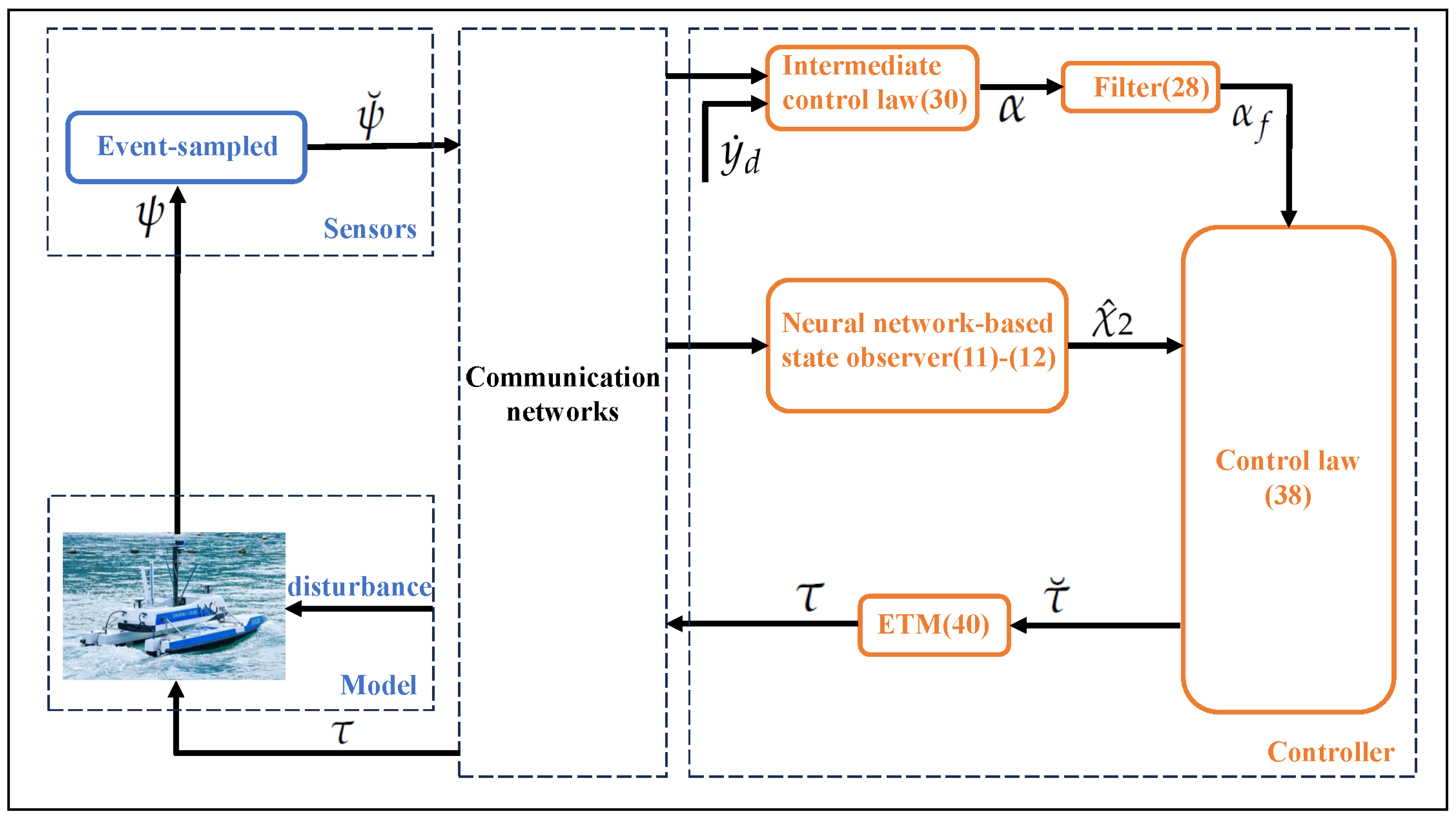
3. Observer Design

3.1. NN-Based State Observer Design

In this subsection, to solve the issue of the constraint of bandwidth, a neural-network-based state observer using only intermittent course data is designed, and the stability analysis is also presented. The detailed processes are presented below.

From (2), the nonlinear model of Norbbin can be rewritten as

$$\begin{array}{c}\hfill \left\{\begin{array}{c}{\dot{\chi }}_1={\chi }_2\hfill \\ {\dot{\chi }}_2=H\left({\chi }_2,\tau \right)+d\hfill \end{array}\right.\end{array}$$

(8)

Here, $H({\chi }_2,\tau )=f\left({\chi }_2\right)+b\tau$. According to Assumption 1, one can establish that $H({\chi }_2,\tau )$ is unknown. In addition, recalling Lemma 1, one can see that $H({\chi }_2,\tau )$ can be approximated by RBF-NN ${\vartheta }^{*}T\xi \left(x\right)$, i.e.,

$$\begin{array}{c}\hfill H\left(s\right)={\vartheta }^{*T}\xi \left(s\right)+{\epsilon }_h\end{array}$$

(9)

where $s={[x^T,\tau ]}^T$ and ${\epsilon }_h$ is the approximate error, which satisfies $|{\epsilon }_h| \le {\overline{\epsilon }}_h$. Furthermore, one can obtain

$$\begin{array}{c}\hfill \left\{\begin{array}{c}{\dot{\chi }}_1={\chi }_2\hfill \\ {\dot{\chi }}_2={\vartheta }^{*T}\xi \left(s\right)+d_h\hfill \end{array}\right.\end{array}$$

(10)

where $d_h=d+{\epsilon }_h$.

According to (10), design the following the NN-based state observer:

$$\begin{array}{c}\hfill \left\{\begin{array}{c}{\dot{\widehat{\chi }}}_1={\widehat{\chi }}_2+k_1\left({\breve{\chi }}_1-{\widehat{\chi }}_1\right)\hfill \\ \dot{\mu }={\widehat{\vartheta }}^T\xi \left(\widehat{s}\right)+k\left({\breve{\chi }}_1-{\widehat{\chi }}_1\right)\hfill \\ {\widehat{\chi }}_2=\mu +k_2({\breve{\chi }}_1-{\widehat{\chi }}_1)\hfill \end{array}\right.\end{array}$$

(11)

with the adaptive law

$$\begin{array}{c}\hfill \dot{\widehat{\vartheta }}=\mathrm{\Lambda }\left({\xi }^T\left(\widehat{s}\right)\left({\breve{\chi }}_1-{\widehat{\chi }}_1\right)-\eta \widehat{\vartheta }\right)\end{array}$$

(12)

where ${\breve{\chi }}_1=\breve{\psi }$ and $\widehat{s}={[x^T,\tau ]}^T$; ${\widehat{\chi }}_1$, ${\widehat{\chi }}_2$ and $\widehat{\vartheta }$ are, respectively, the estimates of ${\chi }_1$, ${\chi }_2$ and $\vartheta$; k, $\eta$, $k_1$, and $k_2$ are the design parameters and $\mathrm{\Lambda }$ is a design matrix.

Remark 5.

The CKC of USVs under a network environment is susceptible to influences from various sources. Under the influence of a network environment and an external environment, the course and yaw data collected by the sensors of USVs are difficult to continuously transmit to the control center at the shore end. Then, the continuous transmission of course and yaw data is the key to ensuring the safety of the course of USVs. To do this, an observer is undoubtedly an effective tool. The observer can be used to improve the accuracy of the transmitted data, thus improving the control performance. At the same time, the observer can also indirectly obtain the signal of $\dot{\psi }$ using the intermittent course data of the USV, which not only saves the cost of installing yaw sensors, but also greatly improves the efficiency of yaw data transmission. Nowadays, there are many kinds of observers, such as state observers, disturbance observers [27], sliding mode observers [28], extended state observers [29], and so on. All of these observers have the function of reconstructing the uncertain state signals inside the system, but they all have to be based on the assumption that the course and yaw are continuous, which undoubtedly makes the work lose effectiveness. Therefore, an NN–SO (11) is designed to resolve the lose effectiveness problem, which does not depend on continuous course data.

Remark 6.

In references [30,31,32,33], several various observers are also designed to achieve the refactoring of the system state, in which the signal ${\breve{\chi }}_1$ must be continuous. In addition, the control gain b must be known if the observer [30,31,32,33] is employed. From (11) and (12), the difference between the proposed observer and the existing observer is that ${\breve{\chi }}_1$ can be discontinuous, which imples that the proposed observer is more practical.

Let ${\tilde{\chi }}_1={\chi }_1-{\widehat{\chi }}_1$, ${\tilde{\chi }}_2={\chi }_2-{\widehat{\chi }}_2$ and $\tilde{\vartheta }=\vartheta -\widehat{\vartheta }$. ${\tilde{\chi }}_1$, ${\tilde{\chi }}_2$, and $\tilde{\vartheta }$ are the estimate errors of ${\chi }_1$, ${\chi }_2$ and $\vartheta$, respectively. And then, the observer error dynamic can be rewritten as

$$\begin{array}{c}\hfill \left\{\begin{array}{c}{\dot{\tilde{\chi }}}_1={\tilde{\chi }}_2-k_1{\tilde{\chi }}_1-k_1\left({\breve{\chi }}_1-{\chi }_1\right)\hfill \\ {\dot{\tilde{\chi }}}_2={\tilde{\vartheta }}^T\xi \left(\widehat{s}\right)+{\rho }_d-k_2{\tilde{\chi }}_2+k_2{\chi }_2-\left(k-k_1{k}_2\right){\tilde{\chi }}_1-\left(k-k_1{k}_2\right)\left({\breve{\chi }}_1-{\chi }_1\right)\hfill \end{array}\right.\end{array}$$

(13)

where ${\rho }_d={\tilde{\vartheta }}^T\left(\xi \left(s\right)-\xi \left(\widehat{s}\right)\right)+d_h$.

Remark 7.

Due to $\forall t\in [t_{\kappa },t_{\kappa +1}),\dot{\breve{\psi }}\left(t\right)=0$, ${\dot{\breve{\chi }}}_1$ will not appear in (13). In addition, the differential term of ${\dot{\widehat{\chi }}}_2$ is not involved in the design process of a NN-based state observer (11), and ${\dot{\breve{\chi }}}_1$ will only appear in the theoretical derivation and stability analysis. Moreover, we will design filters in the control law design to filter the pulse signal that may appear.

3.2. Stability Analysis of State Observer Design

Theorem 1.

For the CKC system (1), under Assumptions 1–3, the NN-based observer (10) with the adaptive law (11) can estimate the states of the system (1) if the design parameters ι, k, η, $k_1$, $k_2$, and Λ can guarantee the following conditions:

$$\begin{array}{c}\hfill \left\{\begin{array}{c}k{k}_1>\iota -k\hfill \\ k_2>2(l+k)\hfill \\ \eta >2+0.5a^{-1}\hfill \end{array}\right.\end{array}$$

(14)

Proof. 

Consider the following Lyapunov function for the NN-based state observer

$$\begin{array}{c}\hfill L_{V_o}=\frac{k}{2}{\tilde{\chi }}_1^2+\frac{1}{2}{\tilde{\chi }}_2^2+\frac{1}{2}{\tilde{\vartheta }}^T{\mathrm{\Lambda }}^{-1}\tilde{\vartheta }\end{array}$$

(15)

Differentiating $L_{Vo}$ and using (13), yield

$$\begin{array}{cc}\hfill {\dot{L}}_{Vo}=& -k{k}_1{\tilde{\chi }}_1^2-k{k}_1{\tilde{\chi }}_1\left({\breve{\chi }}_1-{\chi }_1\right)-k_2{\tilde{\chi }}_2^2+\left({\tilde{\chi }}_2-{\tilde{\chi }}_1\right){\tilde{\vartheta }}^T\xi \left(\widehat{s}\right)+\eta {\tilde{\vartheta }}^T\widehat{\vartheta }+{\rho }_d{\tilde{\chi }}_2\hfill \\ \hfill & -{\tilde{\vartheta }}^T\xi \left(\widehat{s}\right)\left({\breve{\chi }}_1-{\chi }_1\right)+k_2{\chi }_2{\tilde{\chi }}_2+k_1{k}_2{\tilde{\chi }}_1{\tilde{\chi }}_2-\left(k-k_1{k}_2\right)\left({\breve{\chi }}_1-{\chi }_1\right){\tilde{\chi }}_2\hfill \end{array}$$

(16)

According to the ETM (3), one has $|{\breve{\chi }}_1-{\chi }_1|\ge \beta$ for $\forall t\in [t_f,t_{f+1})$. In addition, from the feature of the basis function $\xi \left(\widehat{s}\right)$, one has $\parallel \xi \left(\widehat{s}\right)\parallel \le \sqrt{\iota }$. Furthermore, according to Assumption 2, one can obtain $|{\rho }_d|\le \varsigma$ with $\varsigma$ being a constant. In practice, the steering $\delta$ is a constraint, which implies that ${\chi }_2$ satisfies $|{\chi }_2|\le \theta$ with $\theta$ being a constant. Therefore, the following inequalities hold using Young’s inequality [25]:

$$\begin{array}{c}\hfill -k{k}_1{\tilde{\chi }}_1\left({\breve{\chi }}_1-{\chi }_1\right)\le \frac{k{k}_1}{2}{\tilde{\chi }}_1^2+\frac{k{k}_1}{2}{\beta }^2\end{array}$$

(17)

$$\begin{array}{c}\hfill \left({\tilde{\chi }}_1-{\tilde{\chi }}_2\right){\tilde{\vartheta }}^T\xi \left(\widehat{s}\right)\le \frac{l}{2}\left({\tilde{\chi }}_2^2+{\tilde{\chi }}_1^2\right)+{\parallel \tilde{\vartheta }\parallel }^2\end{array}$$

(18)

$$\begin{array}{c}\hfill {\tilde{\vartheta }}^T\xi \left(\widehat{s}\right)\left({\breve{\chi }}_1-{\chi }_1\right)\le \frac{1}{4a}{\parallel \tilde{\vartheta }\parallel }^2+a\iota {\beta }^2\end{array}$$

(19)

$$\begin{array}{c}\hfill {\rho }_d{\tilde{\chi }}_2\le \frac{1}{4}{\tilde{\chi }}_2^2+4{\varsigma }^2\end{array}$$

(20)

$$\begin{array}{c}\hfill {\tilde{\vartheta }}^T\widehat{\vartheta }\le -\frac{1}{2}\parallel \tilde{\vartheta }{\parallel }^2+\frac{1}{2}{\parallel \vartheta \parallel }^2\end{array}$$

(21)

$$\begin{array}{c}\hfill k{\tilde{\chi }}_1{\tilde{\chi }}_2\le \frac{k}{2}{\tilde{\chi }}_1^2+\frac{k}{2}{\tilde{\chi }}_2^2\end{array}$$

(22)

$$\begin{array}{c}\hfill k_1{k}_2\left({\breve{\chi }}_1-{\chi }_1\right){\tilde{\chi }}_2\le \frac{k_2}{4}{\tilde{\chi }}_2^2+k_2{k}_1^2{\beta }^2\end{array}$$

(23)

where a is a design parameter.

Using (17)–(23), (16) can be rewritten as

$$\begin{array}{cc}\hfill {\dot{L}}_{Vo}\le & -\frac{k{k}_1-\iota -k}{2}{\tilde{\chi }}_1^2-\frac{k_2-2\iota -2k}{4}{\tilde{\chi }}_2^2-\left(\frac{\eta -2}{2}-\frac{1}{4a}\right)\parallel \tilde{\vartheta }{\parallel }^2+\frac{\eta }{2}{\parallel \vartheta \parallel }^2\hfill \\ \hfill & +4{\varsigma }^2+a\iota {\beta }^2+k_2{k}_1^2{\beta }^2+\frac{k{k}_1}{2}{\beta }^2\hfill \\ \hfill \le & -\phi L_{Vo}+\varpi \hfill \end{array}$$

(24)

where $\phi =\min \left\{k{k}_1-\iota -k,\frac{k_2-2\iota -2k}{2},\left(\eta -2-\frac{1}{2a}\right){\lambda }_{\min }\left(\mathrm{\Lambda }\right)\right\}$ and $\varpi =\frac{\eta }{2}{\parallel \vartheta \parallel }^2+4{\varsigma }^2+a\iota {\beta }^2+k_2{k}_1^2{\beta }^2+\frac{k{k}_1}{2}{\beta }^2$. Recalling (24), one can obtain

$$\begin{array}{c}\hfill L_{V_o}\le -\left(\frac{\varpi }{\phi }-L_{V_o}\left(0\right)\right)\exp (-\phi t)+\frac{\varpi }{\phi }\end{array}$$

(25)

where $L_{V_o}\left(0\right)$ is the initial value of $L_{Vo}$. This implies that $L_{Vo}$ is bounded and its upper bound can be adjusted to be as small as desired. Furthermore, from (15), one can understand that ${\tilde{\chi }}_1$, ${\tilde{\chi }}_2$, and $\tilde{\vartheta }$ are bounded, which indicates that the NN-based state observer (10) can estimate the states of the CKC system (1) in real time as long as Equation (24) can be held. Thus, Theorem 1 is proved. □

4. Control Design

Here, the control law for the CKC system is presented using the backstepping design framework. To avoid the design obstacle caused by the ESM in the control design, a filter is introduced. In addition, to handle the unknown nonlinear term and external disturbance, an indirect adaptive NN is developed, in which there is one unknown constant to be updated online.

4.1. Control Law Design

The following error variables are defined before the control design:

$$\begin{array}{c}\hfill s_1={\chi }_1-y_d\end{array}$$

(26)

$$\begin{array}{c}\hfill s_2={\chi }_2-\alpha \end{array}$$

(27)

where $\alpha$ is obtained by filtering through the intermediate control law ${\alpha }_f$. Here, the filter version $\alpha$ is generated by

$$\begin{array}{c}\hfill t_f\dot{\alpha }+\alpha ={\alpha }_f\end{array}$$

(28)

where $t_f$ is the filter constant.

Differentiating $s_1$ and using (2), one can obtain

$$\begin{array}{c}\hfill {\dot{s}}_1={\chi }_2-{\dot{y}}_d\end{array}$$

(29)

Furthermore, design the following intermediate control law without an event sample ${\overline{\alpha }}_f=-k_1{s}_1+{\dot{y}}_r$, where $k_1>0$ is a design constant. According to the ETM (3), one knows that $s_1$ is unavailable, i.e., ${\overline{\alpha }}_f$ is also unavailable. To do this, let ${\breve{s}}_1={\breve{\chi }}_1-y_d$. From (25), one can obtain $s_1={\chi }_1-{\breve{\chi }}_1+{\breve{s}}_1$. In this case, the intermediate control law ${\alpha }_f$ can be designed as

$$\begin{array}{c}\hfill {\alpha }_f=-k_1{\breve{s}}_1+{\dot{y}}_r\end{array}$$

(30)

Substituting (30) into (29) yields

$$\begin{array}{c}\hfill {\dot{s}}_1=s_2+\tilde{\alpha }-k_1{\widehat{s}}_1\end{array}$$

(31)

where $\tilde{\alpha }=\alpha -{\alpha }_f$.

Remark 8.

In the backstepping design method, there is a drawback, i.e., each step requires the derivation of virtual control law. This can lead to a “differential explosion”. Therefore, dynamic surface control technology was developed. Its core idea is to add a first-order filter to each step of the backstepping design, and to convert the differential operation in the backstepping method into simple algebraic operations. This method cannot only reduce the computational complexity, but also avoid the “differential explosion”. To do this, the first-order filter (28) is introduced, which is endowed with a double efficacy, i.e., the control design obstacles caused by ${\dot{\breve{\chi }}}_1$ can be resolved and the control design is also simplified.

Remark 9.

From (3) and (30), one can understand that ${\alpha }_f$ is non-smooth, since ${\breve{\chi }}_1$ is the event-sampled data, which implies that ${\alpha }_f$ is not derivable. Under the backstepping design framework, ${\alpha }_f$ needs to be derivable. In this context, one introduces the filter (28), and the differentiation operation of ${\alpha }_f$ can be removed. As a result, the design obstacle caused by the ESM (3) can be solved.

Differentiating $s_2$ and using (2), one can obtain

$$\begin{array}{c}\hfill {\dot{s}}_2=f\left({\chi }_2\right)+b\tau +d-\dot{\alpha }\end{array}$$

(32)

Let $L=f\left({\chi }_2\right)-\dot{\alpha }+d+s_1$. According to Assumptions 1 and 2, one has that L is unavailable. Furthermore, from Lemma 1, one can obtain

$$\begin{array}{c}\hfill f\left({\chi }_2\right)-\dot{\alpha }={\vartheta }^{*}T\xi \left(x\right)+\epsilon \end{array}$$

(33)

where $x={[{\chi }_2,\dot{\alpha }]}^T$. And then, implementing the following operation for L, one has

$$\begin{array}{c}\hfill \left|L\right|=\left|{\vartheta }^{*}T\xi \left(x\right)+s_1+\epsilon +d\right|\le \theta \varphi \left(x\right)\end{array}$$

(34)

where $\theta =\max \left\{∥{\vartheta }^{*}∥,|\epsilon +d|,1\right\}$ and $\phi \left(x\right)=\parallel \xi \left(x\right)\parallel +\left|s_1\right|+1$. Furthermore, using (32)–(34), one can get

$$\begin{array}{c}\hfill s_2{\dot{s}}_2\le \left|s_2\right|\theta \phi \left(x\right)+b\tau -s_1{s}_2\end{array}$$

(35)

According to Lemma 3, one can get

$$\begin{array}{c}\hfill \left|s_2\right|\theta \phi \left(x\right)\le \theta s_2\phi \left(x\right)\tanh \left(\frac{s_2\phi \left(x\right)}{\sigma }\right)+0.2785\theta \sigma \end{array}$$

(36)

where $\sigma >0$ is a parameter defined by the user. Using (35) and (36), one can obtain

$$\begin{array}{c}\hfill s_2{\dot{s}}_2\le \theta s_2\phi \left(x\right)\tanh \left(\frac{s_2\phi \left(x\right)}{\sigma }\right)+0.2785\theta \sigma +s_{2}b\tau -s_1{s}_2\end{array}$$

(37)

Design the following control law:

$$\begin{array}{c}\hfill \breve{\tau }=-k_2{s}_2-\widehat{\theta }\phi \left(x\right)\tanh \left(\frac{s_2\phi \left(x\right)}{\sigma }\right)\end{array}$$

(38)

the adaptive law,

$$\begin{array}{c}\hfill \dot{\widehat{\theta }}=ϵs_2\phi \left(x\right)\tanh \left(\frac{s_2\phi \left(x\right)}{\sigma }\right)-c\widehat{\theta }\end{array}$$

(39)

and the ETM,

$$\begin{array}{c}\tau \left(t\right)=\breve{\tau }\left(t_{\ell }\right)\forall t\in [t_{\ell },t_{\ell +1})\ell \in \mathrm{N}\hfill \\ t_{t+1}=\inf \left\{t>t_{\ell }\left|\right|z\mid \ge \gamma \right\}\hfill \end{array}$$

(40)

where $k_2$, $ϵ$, c and $\gamma$ are the design parameters, and $z=\tau -\breve{\tau }$ is the measurement error.

More specifically, to illustrate the proposed control scheme more intuitively and clearly, the control system principle block diagram of USVs under a network environment is shown in Figure 1.

4.2. Stability Analysis of Control Law

According to the design above, one can summarize a theorem as follows.

Theorem 2.

Considering the CKC model described by (1), under Assumptions 1–3 and the ESM (3), the CLCS, consisting of the NN–SO (11), (12), filter (28), intermediate control law (30), control law (38), (39), and ETM (40), has the following features:

1.

All signals in the CLCS are bounded;

2.

This can avoid the Zeno behavior.

Proof. 

Consider the following Lyapunov function for CLCS:

$$\begin{array}{c}\hfill L_{Vc}=\frac{1}{2}{s}_1^2+\frac{1}{2}{s}_2^2+\frac{1}{2}{\tilde{\alpha }}^2+\frac{1}{2ϵb}{(\theta -b\widehat{\theta })}^2\end{array}$$

(41)

Differentiating $L_{Vc}$ and using (28), (31), and (37)–(39), one can obtain

$$\begin{array}{cc}\hfill {\dot{L}}_{Vc}\le & s_1\left(s_2+\tilde{\alpha }-k_1\breve{s}\right)+s_2\left((\theta -b\widehat{\theta })\phi \left(x\right)\tanh \left(\frac{s_2\phi \left(x\right)}{\sigma }\right)-s_1+bz-b{k}_2{s}_2\right)\hfill \\ \hfill & +\tilde{\alpha }\dot{\tilde{\alpha }}-(\theta -b\widehat{\theta })\left(s_2\phi \left(x\right)\tanh \left(\frac{s_2\phi \left(x\right)}{\sigma }\right)-\frac{c}{ϵ}\widehat{\theta }\right)+0.2785\sigma \hfill \\ \hfill \le & s_1\left(\tilde{\alpha }-k_1\breve{s}\right)+s_{2}bz-b{k}_2{s}_2^2+\tilde{\alpha }\dot{\tilde{\alpha }}+\frac{c}{ϵ}\widehat{\theta }(\theta -b\widehat{\theta })+0.2785\sigma \hfill \end{array}$$

(42)

Due to $\tilde{\alpha }=\alpha -{\alpha }_f$, one can understand that $\dot{\tilde{\alpha }}=\dot{\alpha }-\dot{{\alpha }_f}$ and $\dot{\alpha }=-\frac{\tilde{\alpha }}{t_f}$. According to Assumptions 3 and [34], there exists a positive constant $\varpi$ satisfying $|{\dot{\alpha }}_f|\le \varpi$. Furthermore, one can obtain

$$\begin{array}{c}\hfill \tilde{\alpha }\dot{\tilde{\alpha }}\le -\left(\frac{1}{t_f}-\frac{1}{2}\right){\tilde{\alpha }}^2+\frac{1}{2}{\varpi }^2\end{array}$$

(43)

From $s_1={\chi }_1-{\breve{\chi }}_1+{\breve{s}}_1$ and the ESM, one can obtain

$$\begin{array}{c}\hfill -s_1\breve{s}=-s_1^2+s_1\left({\chi }_1-{\widehat{\chi }}_1\right)\le -\frac{3}{4}{s}_1^2+{\beta }^2\end{array}$$

(44)

In addition, according to the ETM (40), one can obtain $\left|z\right|\le \gamma$. Furthermore, one has

$$\begin{array}{c}\hfill s_{2}bz\le \frac{k_{2}b}{4}{s}_2^2+\frac{b{\gamma }^2}{k_2}\end{array}$$

(45)

Using Young’s inequation, one obtains

$$\begin{array}{c}\hfill s_1\tilde{\alpha }\le \frac{1}{2}{s}_1^2+\frac{1}{2}{\tilde{\alpha }}^2\end{array}$$

(46)

$$\begin{array}{c}\hfill \widehat{\theta }(\theta -b\widehat{\theta })\le -\frac{{(\theta -b\widehat{\theta })}^2}{2b}+\frac{{\theta }^2}{2b}\end{array}$$

(47)

Substituting (43)–(47) into (42) yields

$$\begin{array}{cc}\hfill {\dot{L}}_{Vc}\le & -\left(\frac{3k_1}{4}-\frac{1}{2}\right)s_1^2-\frac{3b{k}_1}{4}{s}_2^2-\left(\frac{1}{t_f}-\frac{1}{2}\right){\tilde{\alpha }}^2-\frac{c}{2bϵ}{(\theta -b\widehat{\theta })}^2\hfill \\ \hfill & +\frac{1}{2}{\varpi }^2+k_1{\beta }^2+\frac{b{\gamma }^2}{k_2}+\frac{c{\theta }^2}{2bϵ}+0.2785\sigma \hfill \\ \hfill \le & -\varphi L_{Vc}+\rho \hfill \end{array}$$

(48)

where $\phi =\min \left\{\left(\frac{3k_1}{2}-1\right),\frac{3b{k}_1}{2},\left(\frac{1}{t_f}-\frac{1}{2}\right),c\right\}$ and $\rho =\frac{1}{2}{\varpi }^2+k_1{\beta }^2+\frac{b{\gamma }^2}{k_2}+\frac{c{\theta }^2}{2bϵ}+0.2785\sigma$. Solving (48), one can obtain $L_{Vc}\le \left(\frac{\rho }{\varphi }-L_{Vc}\left(0\right)\right)\exp (-\varphi t)+\frac{\rho }{\varphi }$, with $L_{Vc}\left(0\right)$ being the initial value of $L_{Vc}$, which means that $L_{Vc}=\frac{\rho }{\varphi }$ as $t⟶\infty$. Furthermore, from (41), one can determine the boundedness of $s_1$, $s_2$, $\tilde{\alpha }$ and $\theta -b\widehat{\theta }$. Furthermore, from Assumption 3, one determines the boundedness of ${\chi }_1$ and ${\breve{s}}_1$, and then the boundedness of ${\dot{\alpha }}_f$, ${\alpha }_f$ and $\alpha$ according to (26) and (28). In addition, one can understand that ${\chi }_2$ is bounded, and $\phi \left(x\right)$ is also bounded due to the boundedness of $s_2$, ${\chi }_2$, and ${\dot{\alpha }}_f$. Because of the boundedness of $\phi \left(x\right)$, $s_2$, and $\widehat{\theta }$, one can determine the boundedness of $\breve{\tau }$, that is, $\tau$ is also bounded from the ETM (40). Therefore, all signals in the CLCS are bounded.

According to (3) and (39), for $\forall t\in [t_{\kappa },t_{\kappa +1})$ and $\forall t\in [t_{\ell },t_{\ell +1})$, $\breve{\psi }\left(t\right)$ and $\tau \left(t\right)$ are in the hold phase, which implies that they are constant. That is, $\forall t\in [t_{\kappa },t_{\kappa +1})$ and $\forall t\in [t_{\ell },t_{\ell +1})$, $\dot{\breve{\psi }}\left(t\right)=0$ and $\dot{\tau }\left(t\right)$. Taking the time derivative of $e_{\phi }$ and z, one can obtain

$$\begin{array}{c}\hfill \left\{\begin{array}{c}\hfill \frac{d|e_{\psi }|}{dt}\le |\dot{\psi }-\dot{\breve{\psi }}| \le |\dot{\psi }|\\ \hfill \frac{d\left|z\right|}{dt}\le |\dot{\tau }-\dot{\breve{\tau }}| \le |\dot{\breve{\tau }}|\end{array}\right.\end{array}$$

(49)

According to (1) and (2), one can obtain $\dot{\psi }={\chi }_2$. One can determine the boundedness of ${\chi }_2$, which implies that $\dot{\psi }$ is bounded by $|\dot{\psi }| \le \sigma \dot{\psi }$ with $\dot{\psi }$ being a positive constant. In addition, from (38) and (39), one has

$$\begin{array}{c}\hfill \dot{\breve{\tau }}=\left(\frac{\partial \breve{\tau }}{\partial s_2}+\frac{\partial \breve{\tau }}{\partial \tanh (\ast )}\frac{\partial \tanh (\ast )}{\partial s_2}\right){\dot{s}}_2+\frac{\partial \breve{\tau }}{\partial \widehat{\theta }}{\dot{\widehat{\theta }}}^2+\frac{\partial \breve{\tau }}{\partial \varphi \left(x\right)}\left(\frac{\partial \varphi \left(x\right)}{\partial {\chi }_2}{\dot{\chi }}_2+\frac{\partial \varphi \left(x\right)}{\partial \dot{\alpha }}\ddot{\alpha }\right)\end{array}$$

(50)

Furthermore, from (27), (35), (39), and the boundedness of $\dot{\alpha }$, one can understand that $\dot{\widehat{\theta }}$, ${\dot{\chi }}_2$, and $\ddot{\alpha }$ are bounded, which implies that $\dot{\breve{\tau }}$ is bounded by ${\overline{\tau }}_z$. Therefore, there exist two constants satisfying ${\lim }_{t\to \kappa +1}\left|e_{\psi }\right|={\overline{e}}_{\psi }$ and ${\lim }_{t\to \ell +1}\left|z\right|=\overline{z}$, showing that the inter-execution intervals $\sigma t_{\kappa }=t_{\kappa +1}-t_{\kappa }$ and $\sigma t_{\ell }=t_{\ell +1}-t_{\ell }$ are bounded by $\overline{\kappa }$ and $\overline{\ell }$ for $\forall \kappa ,\ell \in N$, respectively. Therefore, one has $\sigma t_k\ge t_k^{\prime }\ge \frac{{\overline{e}}_{\psi }}{\overline{\kappa }}$ and $\sigma t_{\ell }\ge t_{\ell }^{\prime }\ge \frac{\overline{z}}{\overline{\ell }}$, which indicates that the Zeno behavior [25] can be avoided, i.e., the infinite triggering issue cannot occur. □

Remark 10.

Compared with references [23,24,25,26], we proposed a dual-channel ETM to reduce the transmission of course data and control command. In references [23,24,25,26], the transmission of control commands is reduced by construing an ETM on a C–A channel to achieve the requirement of saving communication resources. To do this, the method proposed in references [23,24,25,26] is effective. However, the authors of references [23,24,25,26] only considered a single channel, and did not consider the data transmission from sensors to controllers under the network environment. Therefore, we not only drew on their experience, but also established an ESM in S–C channel, which is only used to transmit intermittent course data. Moreover, it cannot only ensure the intermittent heading data required by the control design requirements, but also reduce the data transmission to a greater extent and save communication resources.

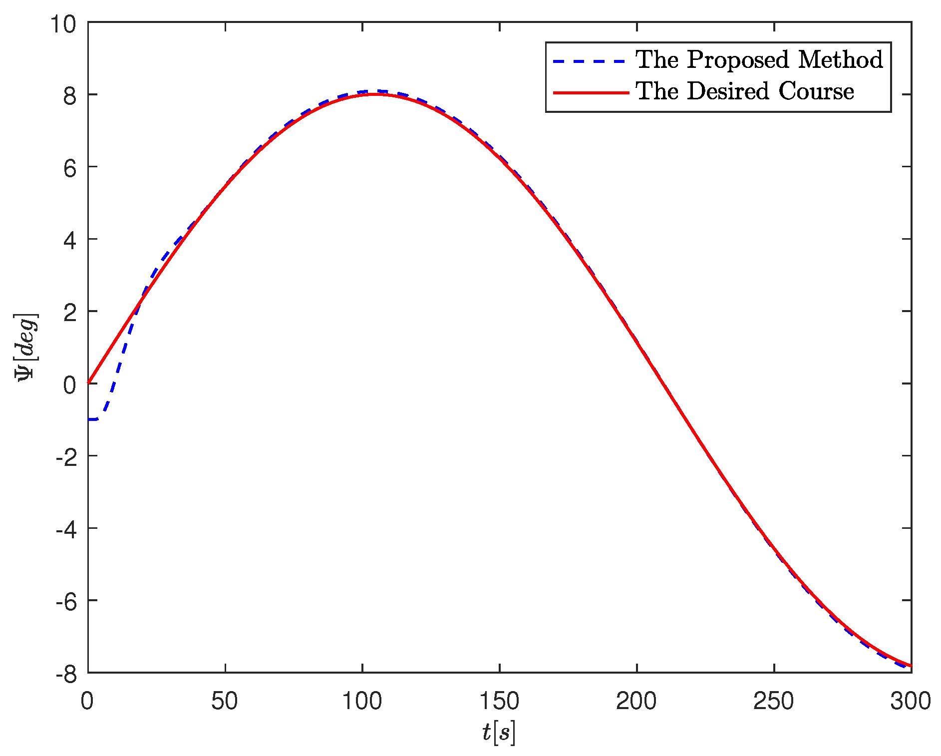
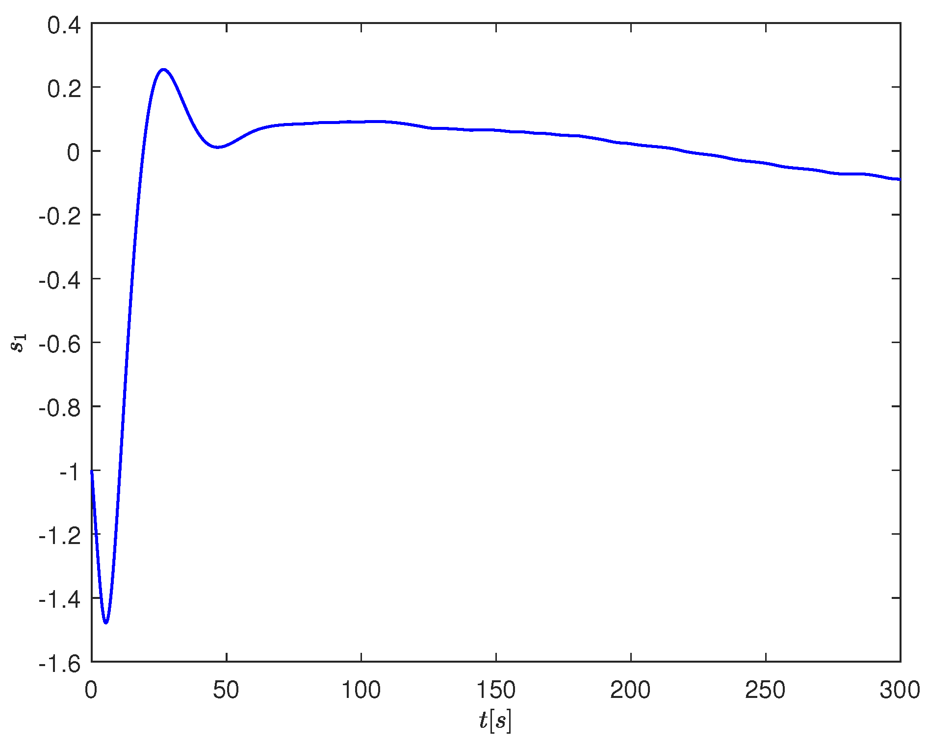
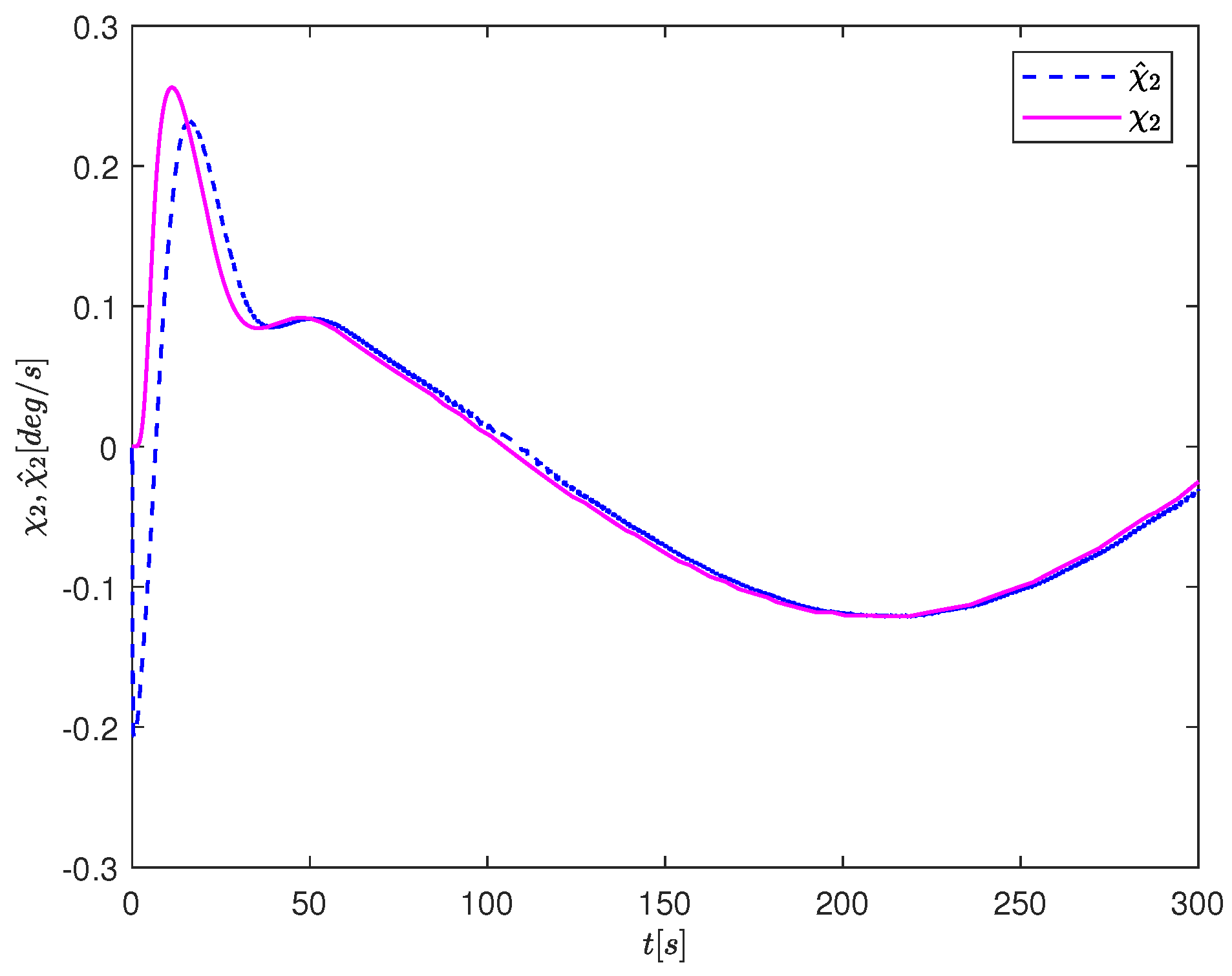
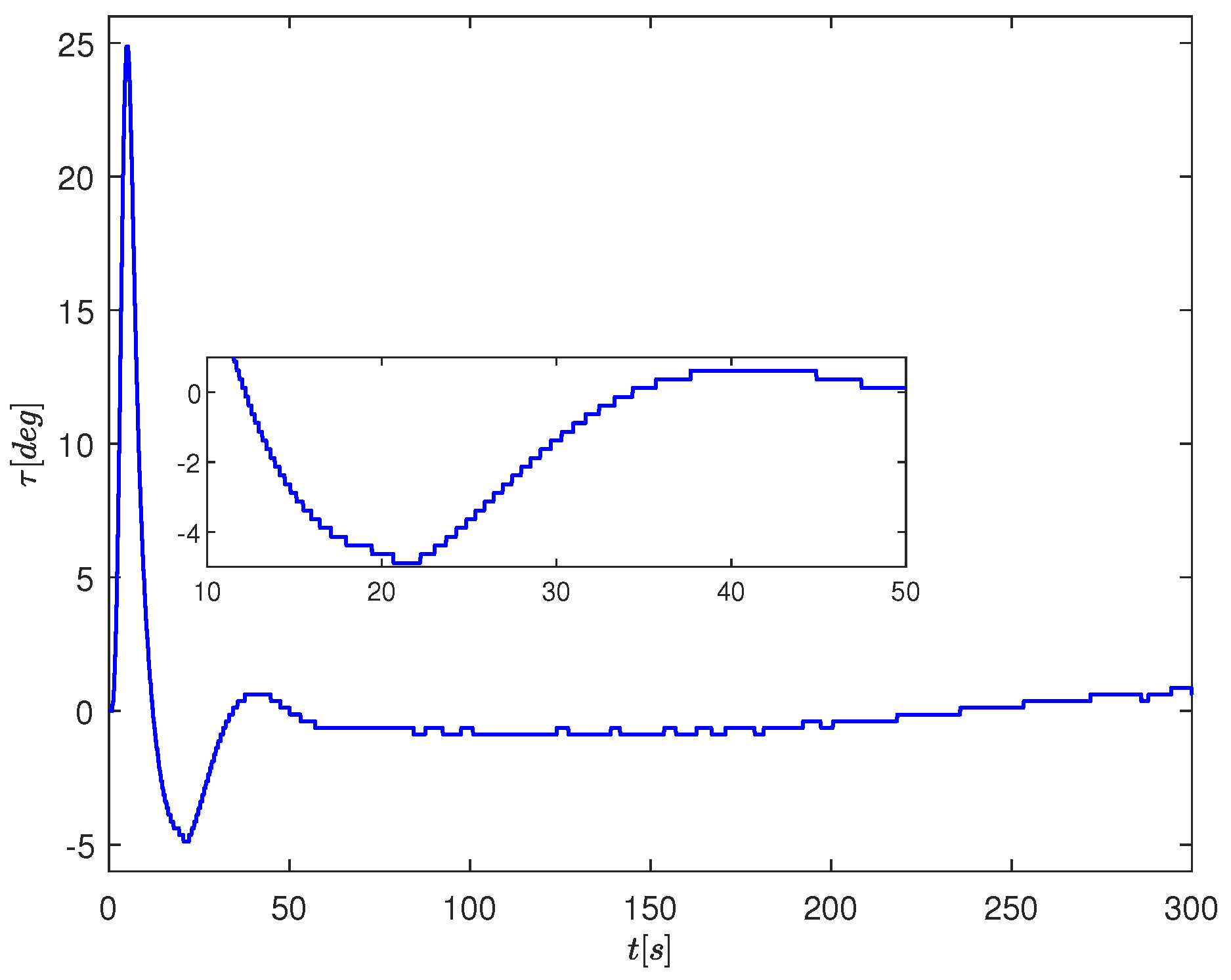
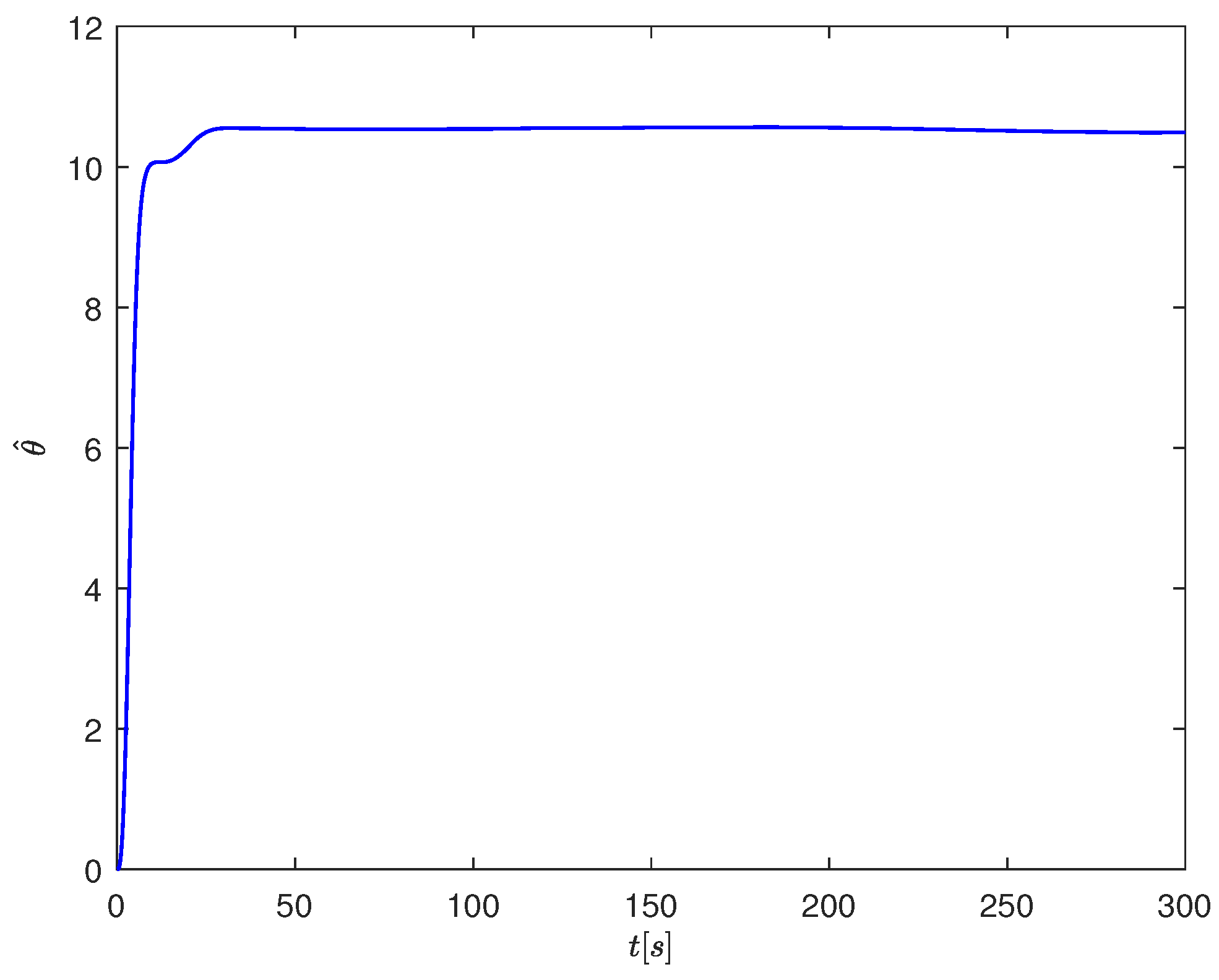
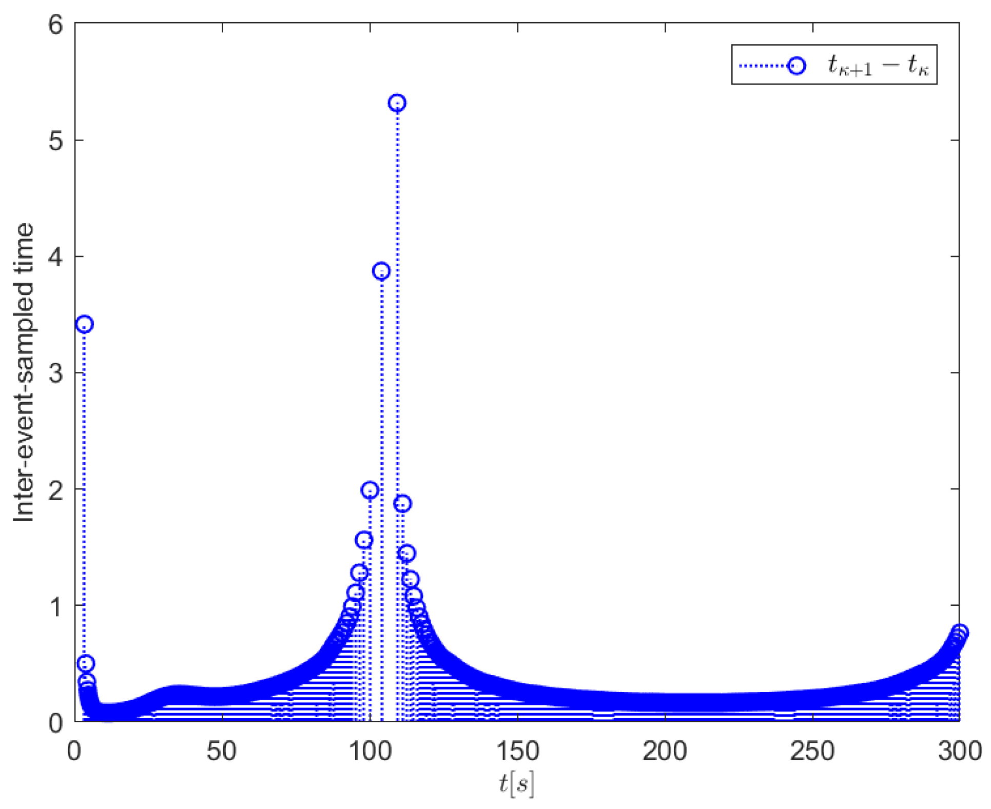
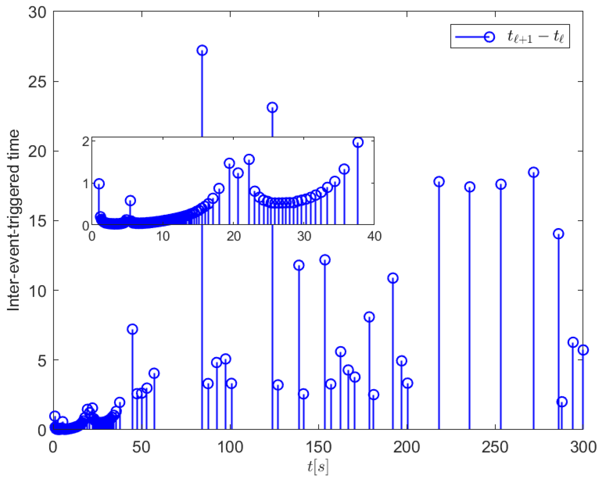
4.3. Simulations

In the simulation, the model parameters of the Norbbin model are $h=-0.00463$, $a_1=1$, $a_3=30$, $b=0.00221$ [12]. The reference course angle $y_d$ is generated using the following dynamic equation $y_d=8sin\left(0.015t\right)$, and the disturbance is chosen as $d=2\left(sin\right(0.2t)+cos(0.3t\left)\right)$. The node number of RBF-NN for $H({\chi }_2,\tau )$ and L is set as 20, the base function centers are evenly spaced in the range [−2 × 2] × [−2 × 2] and all RBF-NN base function widths are set as 1. In addition, the initial states and design parameters are shown in

Table 1. The values of initial states and design parameters.

Index	Items	Value
	$\psi \left(0\right)$	−1
	${\widehat{\chi }}_1$	0
Initial states	${\widehat{\chi }}_2$	0
	$\widehat{\theta }$	0
	$\widehat{\vartheta }$	[0, 0]
Design parameters	k	4
	$k_1$	20
	$k_2$	0.01
	$\eta$	5
	$\mathrm{\Lambda }$	diag ([0.1, 0.1])
	$\beta$	0.02
	$\eta$	5
	$K_1$	0.1
	$K_2$	5
	c	0.1
	$ϵ$	5
	$\sigma$	1
	$t_f$	4
	$\gamma$	0.25

.

The simulation results under the proposed event-triggered control scheme are presented in Figure 2, Figure 3, Figure 4, Figure 5, Figure 6, Figure 7, Figure 8 and Figure 9.

Remark 11.

In this work, the whole CLCS involves several units, such as ESM, NN–SO, and ETM, which leads to a number of design parameters. As a result, the simulation presents some challenges. To address this, we initially determined the design parameters $K_1$ and $K_2$ through trial and error. It should be pointed out that $k{k}_1-\iota -k>0$, $k_2-2\iota -2k>0$ and $\eta >2+{\left(2a\right)}^{-1}$ should be met. Subsequently, one adjusts $K_1$ and $K_2$ to achieve system stability. Following this, one adjusts the other design parameters to meet specific control performance objectives, such as satisfying tracking performance and NN–SO estimation performance. Extensive numerical simulations indicate that, initially, the selection of $K_1$ and $K_2$ is a significant challenge, which relies on the experience of the designer. The relatively large values of $K_1$ and $K_2$ can improve the control performance, but they should not be too large. Otherwise, this causes system oscillation. In the initial phase, it is advisable to endow appropriate values for $K_1$ and $K_2$. And then, according to the control performance, one should increase or decrease the value size appropriately until satisfactory results are achieved. The final tracking performance is influenced by each of the design parameters. When determining these design parameters, it is important to not only adjust one or two parameters separately, but also to tune all the parameters together.

The simulation results under our proposed method are shown in Figure 2, Figure 3, Figure 4, Figure 5, Figure 6, Figure 7, Figure 8 and Figure 9. Specifically, Figure 2 shows that the proposed method is able to force USVs to track the desired course $y_d$ despite equivalent disturbance. Figure 3 presents the varying of the course tracking error. Figure 4 and Figure 5 show the observation performance of the proposed observer for state variables, which is able to achieve the refactoring of the absence of course state data. Figure 6 plots the changing curve of the control input $\tau$, which indicates that the actual steering angle is bounded and reasonable, and that the control input cannot be triggered infinitely within a finite time interval, i.e., the Zeno behavior has been avoided. Figure 7 plots the changing curve of adaptive parameter $\widehat{\theta }$, which indicates that the $\widehat{\theta }$ is bounded. Figure 8 plots the event-sampled instants and times, from which one can understand that the maximal sampling instant is about 5.5 s. Figure 9 shows the event-triggered instant and times in control input channel, from which one can understand that the maximal sampling instant is about 27 s. According to the statistics, the event numbers of sampled events and triggered events are 1251 and 270, respectively. These above results demonstrate that all signals in the CLCS are bounded and that the Zeno behavior has been avoided successfully. Thus, Theorems 1 and 2 are proven.

5. Discussion

In this paper, the issue of course and yaw discontinuity, caused by data transmission and network resources constrains encountered in the CKC of USVs under a network environment, is studied. Firstly, the Norbbin model can more intuitively describe the nonlinear course change of USVs than the Nomoto model. Secondly, under the design framework of backstepping, the technology that can solve the problem of network resource constraints, i.e., ETM, is combined. And the observer technique is used to reconstruct the discontinuity of course data. Finally, the theoretical analysis results show that all the signals in the control system are bounded, using modeling and simulation technology, by choosing appropriate design parameters, as shown in the simulation results in Figure 2, Figure 3, Figure 4, Figure 5, Figure 6, Figure 7, Figure 8 and Figure 9. The simulation results and theoretical analysis of one-to-one correspondence verify the feasibility of the proposed scheme, solving the problem of course keeping control for USVs.

Compared with the existing schemes, the proposed scheme not only uses ETM, but also constructs ESM in an S–A channel, which greatly reduces the data transmission of S–A and C–A channels, reduces the computational workload of the controller, and solves the problem of network resource constraints. In addition, the proposed control scheme is able to achieve the discontinuous reconstruction of course data. However, due to the lack of experimental equipment, it is difficult to perform experimental verification directly. In the network environment, network attack is also one of the problems that cannot be ignored. This is different from external interference, and solving the problem of network attack is the key to ensuring the safe navigation of USVs.

6. Conclusions

In this paper, a dual-channel ETANOFC scheme is proposed for the issue of CKC for USVs under a network environment. It can resolve the issue of network resource constraints by using the ESM and an ETM, both in the S–C and C–A channels. In addition, to solve the course data discontinuity problem caused by ESM, a novel adaptive NN–SO is developed to recover the yaw information, which solves the absence of yaw in the data transmission. In addition, the dynamic surface control technique is employed to implement the backstepping design approach in the control design. The theoretical results indicate that, under the developed control solution, all signals in the CLCS are bounded, and the effectiveness is verified by simulation results.

In the future, the CKC of USVs under a network environment must consider network attack. Addressing network attacks is one of the elements necessary for ensuring the safety of USVs navigation.

References

- Ma, Y.; Hu, M.; Yan, X. Multi-objective path planning for unmanned surface vehicle with currents effects. ISA Trans. 2018, 75, 137–156. [Google Scholar] [CrossRef]
- Ma, Y.; Zhao, Y.; Li, Z.; Bi, H.; Wang, J.; Malekian, R.; Sotel, M. CCIBA*: An improved BA* based collaborative coverage path planning method for multiple unmanned surface mapping vehicles. IEEE Trans. Intell. Transp. Syst. 2022, 23, 19578–19588. [Google Scholar] [CrossRef]
- Shao, G.; Ma, Y.; Malekian, R.; Yan, X.; Li, X. A novel cooperative platform design for coupled USV–UAV systems. IEEE Trans. Ind. Inform. 2019, 15, 4913–4922. [Google Scholar] [CrossRef]
- Gu, N.; Wang, D.; Peng, Z.; Wang, J.; Han, Q. Advances in line-of-sight guidance for path following of autonomous marine vehicles: An overview. IEEE Trans. Syst. Man Cybern. Syst. 2023, 53, 12–28. [Google Scholar] [CrossRef]
- Liu, Z.; Zhang, Y.; Yu, X.; Yuan, C. Unmanned surface vehicles: An overview of developments and challenges. Annu. Rev. Control 2016, 41, 71–93. [Google Scholar] [CrossRef]
- He, Z.; Fan, Y.; Wang, G.; Qiao, S. Finite time course keeping control for unmanned surface vehicles with command filter and rudder saturation. Ocean Eng. 2023, 280, 114403. [Google Scholar] [CrossRef]
- Zhang, G.; Han, J.; Zhang, W.; Yin, Y.; Zhang, L. Finite-time adaptive event-triggered control for USV with COLREGS-compliant collision avoidance mechanism. Ocean Eng. 2023, 285, 115357. [Google Scholar] [CrossRef]
- Fossen, T.I. Handbook of Marine Craft Hydrodynamics and Motion Control; John Wiley & Sons: Trondheim, Norway, 2011. [Google Scholar]
- Er, M.J.; Ma, C.; Liu, T.; Gong, H. Intelligent motion control of unmanned surface vehicles: A critical review. Ocean Eng. 2023, 280, 114562. [Google Scholar] [CrossRef]
- Hu, J.; Ge, Y.; Zhou, X.; Zhou, X.; Liu, S.; Wu, J. Research on the course control of USV based on improved ADRC. Syst. Sci. Control Eng. 2021, 9, 44–51. [Google Scholar] [CrossRef]
- Lai, P.; Liu, Y.; Zhang, W.; Xu, H. Intelligent controller for unmanned surface vehicles by deep reinforcement learning. Phys. Fluids 2023, 35, 037111. [Google Scholar] [CrossRef]
- Islam, M.M.; Siffat, S.A.; Ahmad, I.; Liaquat, M. Robust integral backstepping and terminal synergetic control of course keeping for ships. Ocean Eng. 2021, 221, 108532. [Google Scholar] [CrossRef]
- González-Prieto, J.; Carlos, P.; Yogang, S. Adaptive integral sliding mode based course keeping control of unmanned surface vehicle. J. Mar. Sci. Eng. 2022, 10, 68. [Google Scholar] [CrossRef]
- Hu, S.; Yang, P.; Chang, B. Robust nonlinear ship course-keeping control by H∞ I/O linearization and μ-synthesis. Int. J. Robust Nonlinear Control 2003, 13, 55–70. [Google Scholar] [CrossRef]
- Zheng, Y.; Tao, J.; Sun, Q.; Sun, H.; Sun, M.; Chen, Z. An intelligent course keeping active disturbance rejection controller based on double deep Q-network for towing system of unpowered cylindrical drilling platform. Int. J. Robust Nonlinear Control 2021, 31, 8463–8480. [Google Scholar] [CrossRef]
- Omerdic, E.; Roberts, G.; Vukic, Z. A fuzzy track-keeping autopilot for ship steering. J. Mar. Eng. Technol. 2003, 2, 23–35. [Google Scholar] [CrossRef]
- Xiong, Y.; Pan, L.; Xiao, M.; Xiao, H. Motion control and path optimization of intelligent AUV using fuzzy adaptive PID and improved genetic algorithm. Math. Biosci. Eng. 2023, 20, 9208–9245. [Google Scholar] [CrossRef] [PubMed]
- Zhu, G.; Ma, Y.; Hu, S. Event-Triggered Adaptive PID Fault-Tolerant Control of Underactuated ASVs Under Saturation Constraint. IEEE Trans. Syst. Man Cybern. Syst. 2023, 53, 4922–4933. [Google Scholar] [CrossRef]
- Chen, C.; Evert, L.; Guillaume, D. Experimental study of adaptive course controllers with nonlinear modulators for surface ships in shallow water. ISA Trans. 2023, 134, 417–430. [Google Scholar] [CrossRef] [PubMed]
- Ju, X.; Li, J.; Du, P. A novel non-fragile H∞ fault-tolerant course-keeping control for uncertain unmanned surface vehicles with rudder failures. Ocean Eng. 2023, 280, 114781. [Google Scholar]
- Zhang, G.; Liu, S.; Li, B.; Zhang, X. Robust composite dynamic event-triggered control for multiple USVs with DLLOS guidance. J. Mar. Sci. Eng. 2022, 10, 227. [Google Scholar] [CrossRef]
- Borgers, D.; Heemels, H. Event-separation properties of event-triggered control systems. IEEE Trans. Autom. Control 2014, 59, 2644–2656. [Google Scholar] [CrossRef]
- Zhang, G.; Gao, S.; Li, J.; Zhang, W. Adaptive neural fault-tolerant control for course tracking of unmanned surface vehicle with event-triggered input. Proc. Inst. Mech. Eng. Part J. Syst. Control Eng. 2021, 235, 1594–1604. [Google Scholar] [CrossRef]
- Zhou, L.; Shen, Z.; Nie, Y.; Yu, H. Event-triggered adaptive dynamic programming for optimal tracking control of unmanned surface vessel with input constraints. Trans. Inst. Meas. Control 2023. [Google Scholar] [CrossRef]
- Zhu, G.; Ma, Y.; Li, Z.; Malekian, R.; Sotelo, M. Dynamic event-triggered adaptive neural output feedback control for MSVs using composite learning. IEEE Trans. Intell. Transp. Syst. 2023, 24, 787–800. [Google Scholar] [CrossRef]
- Zhang, J.; Tong, S. Event-Triggered Fuzzy Adaptive Output Feedback Containment Fault-Tolerant Control for Nonlinear Multi-agent Systems against Actuator Faults. Eur. J. Control 2023, 100887. [Google Scholar] [CrossRef]
- Hu, X.; Wei, X.; Han, J.; Zhu, X. Adaptive disturbance estimation and cancelation for ships under thruster saturation. Int. J. Robust Nonlinear Control 2020, 30, 5004–5020. [Google Scholar] [CrossRef]
- Kim, H.; Lee, J. Robust sliding mode control for a USV water-jet system. Int. J. Nav. Archit. Ocean Eng. 2019, 11, 851–857. [Google Scholar] [CrossRef]
- Fan, Y.; Qiu, B.; Liu, L.; Yang, Y. Global fixed-time trajectory tracking control of underactuated USV based on fixed-time extended state observer. ISA Trans. 2023, 132, 267–277. [Google Scholar] [CrossRef]
- Park, B.S.; Kwon, J.W.; Kim, H. Neural network-based output feedback control for reference tracking of underactuated surface vessels. Automatica 2017, 77, 353–359. [Google Scholar] [CrossRef]
- Jia, Z.; Hu, Z.; Zhang, W. Adaptive output-feedback control with prescribed performance for trajectory tracking of underactuated surface vessels. ISA Trans. 2019, 95, 18–26. [Google Scholar] [CrossRef]
- Deng, Y.; Zhang, X. Event-triggered composite adaptive fuzzy output-feedback control for path following of autonomous surface vessels. IEEE Trans. Fuzzy Syst. 2020, 29, 2701–2713. [Google Scholar] [CrossRef]
- Peng, Y.; Wang, D.; Li, T.; Han, M. Output-feedback cooperative formation maneuvering of autonomous surface vehicles with connectivity preservation and collision avoidance. IEEE Trans. Cybern. 2019, 50, 2527–2535. [Google Scholar] [CrossRef] [PubMed]
- Xia, X.; Yang, Z.; Yang, T. Leader–Follower Formation Tracking Control of Underactuated Surface Vehicles Based on Event-Trigged Control. Appl. Sci. 2023, 13, 7156. [Google Scholar] [CrossRef]