Performance Evaluation of an API Stock Exchange Web System on Cloud Docker Containers

Abstract

This study aims to identify the most effective input parameters for performance modelling of container-based web systems. We introduce a method using queueing Petri nets to model web system performance for containerized structures, leveraging prior measurement data for resource demand estimation. This approach eliminates intrusive interventions in the production system. Our research evaluates the accuracy of various formal estimation methods, pinpointing the most suitable for container environments. With the use of a stock exchange web system benchmark for data collection and simulation verification, our findings reveal that the proposed method ensures precise response time parameter accuracy for such architectural configurations.

1. Introduction

Container systems are becoming increasingly popular. Today, many companies are using containerization techniques increasingly to create new applications for the cloud. Therefore, researchers who build performance models (PMs) of modern systems should construct them for containers too. Containerized environments are a new challenge for performance evaluation based on performance engineering (PE). For a performance engineer, it is crucial to utilize effective simulation and estimation techniques. PMs are able to investigate multiple metrics during the design of web systems and are assessed through analytical or simulation methods. Despite several benefits, predicting the performance of a specific system is still a complicated undertaking.

Resource demand is one of the main parameters of the PMs; it needs to be determined in a quantitative analysis [1]. This is the average time that a request spends obtaining a service from the resource, excluding any waiting time. Exact resource demand value establishment is crucial for performance modelling [2,3]. Various factors indicate the resource demand, but measuring it is challenging due to potential measurement interference. Hence, queueing theory-based statistical estimation techniques such as linear regression or Kalman filters are used. The precision of these methods relies on platform-specific parameters, and there is no optimal approach for all cases.

The goal of this paper is performance evaluation based on PMs. The paper makes the following contributions: (1) a scheme for a container-based example stock exchange web system as a benchmark and its experiments, (2) resource demand estimation based on the logs of this system, (3) modelling and performance analysis of PMs, and (4) a comparison of simulation results with experimental results for response time parameter. There are no publicly available works on this functionality for container-based systems. Resource demand estimation approaches are used to build the PMs of a system.

1.1. Motivation

In today’s digital age, individuals frequently interact with a myriad of web applications and cloud servers. These interactions, although convenient, contribute to environmental concerns due to power consumption. Enhancing the efficiency of these systems could help alleviate such environmental impacts. Given the prevalence of container models in data centre systems, understanding their performance through accurate modelling becomes paramount. PMs serve as a predicting tool for system behaviour, with a particular focus on processor resources in this study. To avoid imposing additional load on the CPU during the estimation of its resource demand, we used statistical estimation techniques. By measuring the average response time per request and CPU utilization, we aim to refine our understanding of resource demand values, aligning with our broader goal of optimizing container-based web system performance.

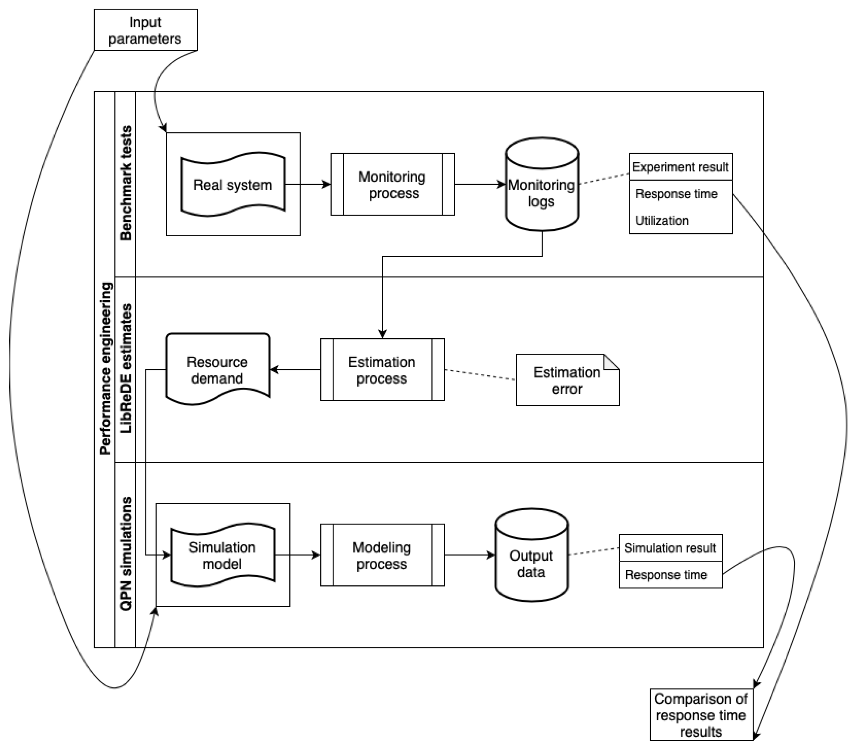
1.2. Performance Evaluation Process

Over time, several approaches to PE have been proposed using diverse formalisms. However, performance evaluation on container-based systems still remains a novel area for exploration. These approaches vary in the models they rely on and the mathematical techniques used. Figure 1 depicts the three various PE processes running in a sequence applied in this approach: experiments (1), estimations (2), and finally simulations (3). In the following, we will discuss each of the individual activities in more detail. The experiments use real servers. We based the benchmark on the Stock Exchange Web System (SEWS) [4] as an application programming interface (API) based on https://www.ibm.com/docs/en/linux-on-systems?topic=descriptions-daytrader-benchmark-application (accessed on 31 August 2023). Then, we prepared the custom Stock Exchange Load Generator (SELG) as the automatic client for SEWS API. To estimate the resource demand, we established a container environment utilizing SEWS and SELG, which produces output data. Therefore, using these data, we could forecast the resource demand in active containers without unnecessary interaction with the software or hardware. Furthermore, the simulation results might serve as an alternative to experimental results. Simulations use dedicated software and equipment (a computer) that are not the actual objects but generate comparable outcomes. In the simulation process, we used an approach that had been previously verified [5].

This article outlines the creation of a PMs for a novel system. We delineated a technique to set the value of the input parameter (resource demand) for PM simulation using the queueing Petri nets (QPNs) formalism. Next, we scrutinized the PMs to derive a response time. We then validated the simulation model using the measured values, utilizing the response time to compare the simulation values with the measured ones.

1.3. Organization

The paper consists of the following parts: (1) preparation of SEWS tests and benchmarks, (2) resource demand estimation based on SEWS logs, (3) PM analysis and simulations, and (4) a comparison of model results to real manufacturing system results.

The remainder of the paper is organized as follows. Section 2 includes the related works. Section 3 introduces SEWS and SELG in container-based architecture and checks the performance with experiments. Section 4 gives the results of resource demand estimation. Section 5 discusses the QPN models and presents the simulation results. Additionally, it includes a comparative analysis of the experiments and simulations. Finally, Section 6 discusses the approach and concludes the paper.

2. Related Work

This section covers the literature review on the subject of PE for web system architectures. Response time is a critical parameter in any performance analyses and has received significant attention in recent years in many PE approaches [6]. Numerous authors have introduced corresponding modelling approaches based on response time [7,8,9,10]. Unfortunately, none of the varied approaches for PE have included container-based systems in their assessment. Although none of the works specifically concentrate on container environments, the concept of using queueing Nets (QNs) [9] or Petri nets (PNs) [11] for web system modelling is not novel. As such, the ideas presented in the papers [9,12,13,14,15], which successfully applied it to other system structures [16] and domains [17], are incorporated in this article. There are PMs [11,17,18,19] based on different formalisms. PE is primarily influenced by the development of computer and communication networks, manufacturing system assessment, and business process analysis. In recent years, numerous studies have centred on web systems, which are highly efficient and can handle a large volume of incoming requests. There are two mathematical formalisms available to address performance evaluation and analysis problems [1,10,20]: QNs and PNs. Queueing methods are a well-established and widely used approach for dealing with limited resources. QNs allow the calculation of the throughput of the subsequent elements of a computing process represented as a network of queueing systems [18]. PNs are a specific type of graph where tokens flow through the network [11]. They can be interpreted as the reallocation of the load [21] within the system under study.

In [15], Krajewska presented a systematic survey of the existing database performance evaluation models based on queueing theory. In [11], probabilistic PNs were proposed. In some cases, we may use a transformation of a UML design [17,22] to a PN model for evaluating performance metrics. Furthermore, we can consider the measured web performance as automatically measured performance metrics [23] and find the best perceived performance as evaluated by the users.

The techniques proposed in [24] and [8] could be helpful in the context of evaluating the performance of web structures. Zatwarnicki et al. [8] developed a two-layer decision-making method for cloud-based web systems using a neuro-fuzzy approach. In [25], the authors presented an engineering perspective for building a meta-model to manage the performance of cloud-native applications. In [24] and [26], a new HTTP request distribution method was proposed for a two-layer architecture consisting of a cluster-based web system and a cloud system. This approach enables efficient processing and predictable quality of service for requests within specified time constraints. The latest models [27] can be used to model HTTP request generators for modern web systems. Recent publications [1,28] demonstrated the use of stochastic formalisms for PMs of web systems and compared their models to the production system performance. QPNs, successful combinations of QNs and PNs formalisms, are used in the main models presented by Rak [29] and Eismann [10], which are also widely used in other areas as shown in [5]. Kounev et al. [13] extended these works by investigating the impact of different factors on performance metrics. Rygielski et al. [28] also studied performance metrics. In [30], an analysis of data package availability in container-based systems was presented, and proposed performance analysis in container-based systems helped identify potential bottlenecks. In [14], a new methodology for modelling production systems was introduced which addresses availability, reliability, and performance issues. When constructing a production system based on architecture and design patterns, it is essential to consider quality attributes such as resilience or trustworthiness, as noted in [31].

Several articles including [7,27,28], and [12] have presented models based only on the native architecture, whereas some authors such as [1,8], and [10] have considered other approaches. These models are validated through experiments, but none of them compared native systems with container architecture or considered systems with multiple processing resources. Our work proposes a formal PE model for container technology, which is the first of its kind, and we gather PM input parameters and benchmark logs from a container-based system, taking into account the performance costs imposed by Docker containers. Most related work focuses on models optimized for different use cases in native or virtualized environments.

The most important related works are described (advantages/disadvantages) in table (

Table 1. The advantages and disadvantages of the related works.

Approach	Advantages	Disadvantages
[2]	Cloud infrastructure; online analysis	The time series segmentation strategy has limitations, especially concerning the selection of thresholds; One-class client
[3]	Cloud infrastructure; The proposed training method incorporates back propagation	Lack of performance analysis
[1]	Container-based infrastructure	Measured model parameters; one-class client
[10]	Cloud infrastructure	Measured model parameters; offline analysis
[28]	Parameter prediction; online analysis;	Native systems
[29]	Multi-class client	Native systems; measured model parameters
This approach	Container-based infrastructure; parameter prediction	One-class client; offline analysis

).

3. Container-Based Web System Architecture and Experiments

In this section, we will present the results obtained from our tests. Testing is an integral part of the application development cycle.

To obtain log traces, we conducted experiments in real environments using our prepared stock exchange benchmark (SEWS) and load generator (SELG). These benchmark tests were conducted in repeatable environments, and we proposed several different experiments to prepare input data for future estimations. Our collection includes 249 traces, with a minimum runtime of 4 h and a maximum of 24 h [32].

The different types of systems are associated with different user behaviours, and our modelling approach differs from other works as we used various system architectures. Benchmark tests were used to obtain values for performance output parameters.

3.1. Container-Based Web System Architecture Approach

During the development of a web application, it is usually created on a local machine, but it may fail when deployed to a cloud production environment. To avoid this problem, we may develop the application in a container system on the cloud, as rebuilding is not required. However, the formal model of such a system cannot be fully studied and exploited [33].

Docker is a tool to run applications on containers, which offers many advantages over other deployment technologies, although Docker containers have less overhead than virtual machines, they still have some, and processes running within a container may not be as fast as those running on the native OS [34].

For our experiments, we deployed SEWS on Docker containers, with the backend servers containing the Django web framework (Python) and an open-source PostgreSQL database accessed through the $psycopg2$ adapter. SELG was executed on a separate container. We required two Docker environments: one for the production system and the another for the load generator.

Containers utilize host OS resources, and multiple applications share the same OS kernel, which means that containerized systems are less isolated than virtual machines. Docker containers are comparable to regular processes running on the same Docker host, with the Docker host being the server on which the Docker daemon runs. Because Docker operates on the same OS as its host, it shares the host kernel, enabling the sharing of host OS resources. Docker adds only one extra layer between the hardware and the web application.

3.2. Hardware Elements

This subsection details the hardware test environment utilized for the analysis, which involved deploying the system on the Docker container platform. Our system comprises a logic tier and a database, with the application (SEWS) deployed as a benchmark (as shown in Figure 2) within a container with a Linux OS to simulate a realistic container setup using the Docker engine in Swarm mode. The request load generator (SELG) was deployed in a separate container. Depending on the test, we used different number of containers (1 (Figure 2a), 5 (Figure 2b) and 10 (Figure 2c)).

We used a pool of containers running on a machine that had: 4, 8, and 12 CPUs; 10, 20, and 30 GB RAM ($Exp.1$: $12-30$ (12 CPU and 30 GB RAM), $Exp.2$: $8-20$, and $Exp.3$: $4-10$ cases), and Linux Debian 10 (Buster) 64-bit OS. We used the standard kernel provided by Linux Debian in version 4.19.0–16. Tables (

Table 2. Multi-container laboratory environment (experiment 1).

Parameter	$\mathit{Exp}.1$
Processors	12
RAM [GB]	30
Container structure ${}^{(}$${}^a$${}^{)}$	$C1$	$C5$	$C10$
Test	$ET1$	$ET2$	$ET3$
$1/Think\_time$	6.242	4.849	3.826
– [req/s] ${}^{(}$${}^b$${}^{)}$
$Think\_time$	0.166	0.207	0.261
– [s]

${}^{(}$${}^a$${}^{)}$ Number of database connections in all cases is equal to 90 per container. ${}^{(}$${}^b$${}^{)}$ Number of clients (workload) in all cases is equal to 90.

,

Table 3. Multi-container laboratory environment (experiment 2).

Parameter	$\mathit{Exp}.2$
Processors	8
RAM [GB]	20
Container structure ${}^{(}$${}^a$${}^{)}$	$C1$	$C5$	$C10$
Test	$ET4$	$ET5$	$ET6$
$1/Think\_time$	66.732	5.009	2.975
– [req/s] ${}^{(}$${}^b$${}^{)}$
$Think\_time$	0.55	0.200	0.337
– [s]

${}^{(}$${}^a$${}^{)}$ Number of database connections in all cases is equal to 90 per container. ${}^{(}$${}^b$${}^{)}$ Number of clients (workload) in all cases is equal to 90.

and

Table 4. Multi-container laboratory environment (experiment 3).

Parameter	$\mathit{Exp}.3$
Processors	4
RAM [GB]	10
Container structure ${}^{(}$${}^a$${}^{)}$	$C1$	$C5$	$C10$
Test	$ET7$	$ET8$	$ET9$
$1/Think\_time$	6.366	3.152	1.644
– [req/s] ${}^{(}$${}^b$${}^{)}$
$Think\_time$	0.164	0.317	0.610
– [s]

${}^{(}$${}^a$${}^{)}$ Number of database connections in all cases is equal to 90 per container. ${}^{(}$${}^b$${}^{)}$ Number of clients (workload) in all cases is equal to 90.

) include the hardware configuration ($ET1-ET9$). A separate network was established to interconnect all the containers. We executed only the required programs for our tests and gathered data on the arrival and execution times of each request and the average CPU utilization during each experiment. SELG measured the benchmark execution times, and we used the $psutil$ library to measure the CPU utilization.

3.3. Software Elements

In the following section, we will provide a description of the software experimentation environments (SEWS and SELG) that were utilized for the evaluation of our approach. Each method necessitates a distinct set of input parameters, which is dependent on the specific test and the underlying system architecture [35]. We carried out several test runs for the different numbers of requests (100,000, 400,000, and 700,000) and varied the number of containers ($C1$, $C5$, and $C10$).

3.3.1. SEWS

To conduct a precise evaluation, we require a benchmark that is specifically designed for the purpose. Our benchmark simulates an online stock exchange system and provides a controlled environment for testing. The benchmark, named SEWS, is modelled after the IBM DayTrader Benchmark, which is designed to represent typical internet commerce applications. SEWS comprises a database and a set of application programming interface (API) endpoints. The API endpoints are designed to function as a web API and include the following endpoints [36]:

• (1) User registration;
• (2) User login and (3) user logout;
• (4) Create a new purchase offer, (5) delete the purchase offer, (6) create a new sale offer, and (7) delete the sale offer;
• (8) Return the list of companies, (9) returns the list of all companies, (10) return details about the company;
• (11) Details of the current user, adding users, and editing the user;
• (12) Returns the current user’s wallet status;
• (13) Returns the list of resources owned by the user, (14) returns the list of active sell/buy offers for a given user, (15) returns the list of completed transactions for a given user, and(16) returns the list of all available actions;
• (17) Allows you to buy stocks at the current price and (18) allows you to sell stocks at the current price;
• (19) Returns the list of all buy and sell orders: active and closed and (20) returns a list of all buy and sell orders for a given action: active and closed.

The SEWS benchmark defines requests that the online stock exchange supports. These requests are divided into two groups: GET and POST type. Both of them use the database.

3.3.2. SELG

To generate a defined load on SEWS resources, we used a load generator called SELG. This tool emulates user behaviour and sends requests to stress the web API. The workload consists of one request class, and during the experiment runs, we collect measurements of the response times of individual requests and resource utilization.

The SELG runs in a separate container, and we used the $psutil$ library to monitor CPU utilization and retrieve information on running processes. We applied a 30 s interval to obtain these measurements. The SELG logs the response time of each request, which we collected with the timestamp. These measurements are used to estimate resource demand.

3.4. Benchmark Tests

This subsection explains the test setup utilized for collecting measurement traces. The real system provides us with the real values of performance parameters and allows us to determine the resource demands. We conducted a series of experiments using an implementation based on the Django (Python) framework and a PostgreSQL database. Django is a set of Python libraries that enables the development of web applications, and PostgreSQL is an open-source database management system designed for web applications.

The backend container maintains a database connection pool, and we ensured that this pool did not cause any additional delays by setting the maximum number of clients to be equal to its size. Refer to tables (Table 2, Table 3 and Table 4) for additional details about the containerized execution environment. Each server runs within its container.

The workload is generated as follows:

• Each request is associated with a real client and represents their behaviour in the system.
• User sends the request to a specified endpoint of SEWS.
• User think time (Think time is defined as the time between the completion of one request and the start of the next request.) between two requests is drawn from an exponential distribution. It is possible to scale the workload by changing user think time [37].
• User behaviour is connected to the possible navigation paths within a scenario.

Due to the lack of traces from the real container system, we used an application benchmark (SEWS) for the prepared scenario instead. Tests scenario:

• User registration;
• Login;
• List of all available stock exchange,;
• User wallet status;
• Purchase of a single stock of the SEWS;
• List of resources owned by the user;
• Sale offers;
• List of the user’s current sale/purchase offers;
• List of completed user transactions.

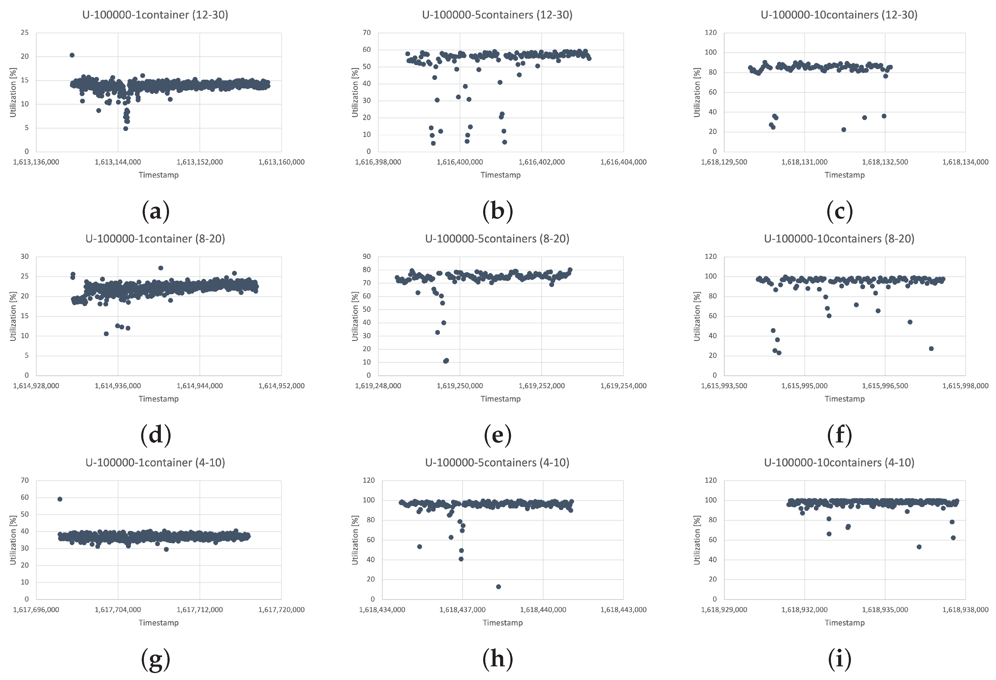
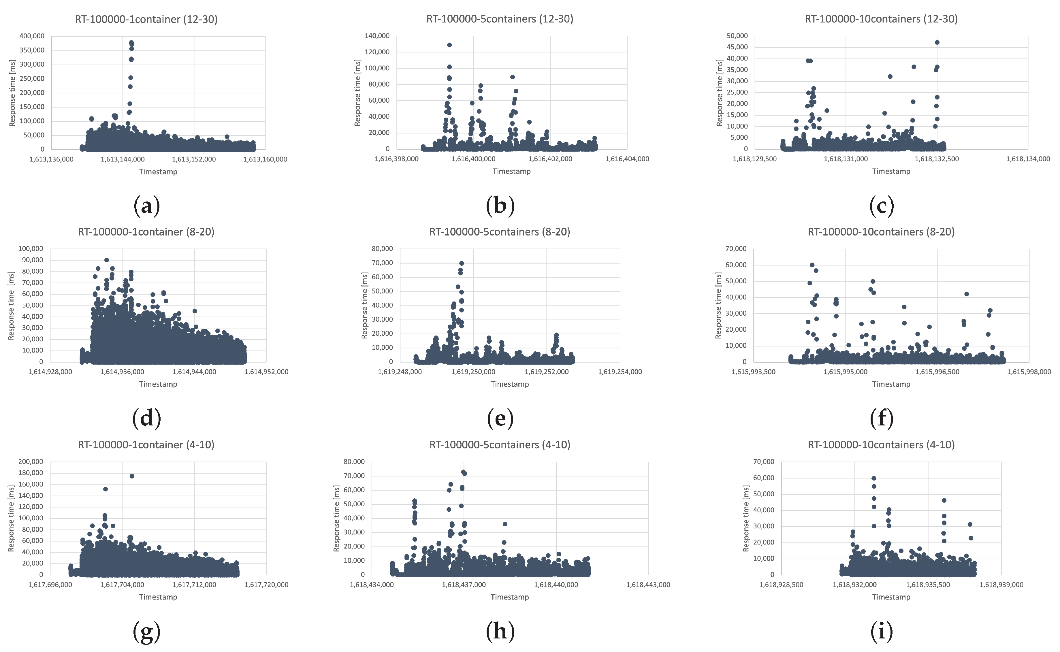
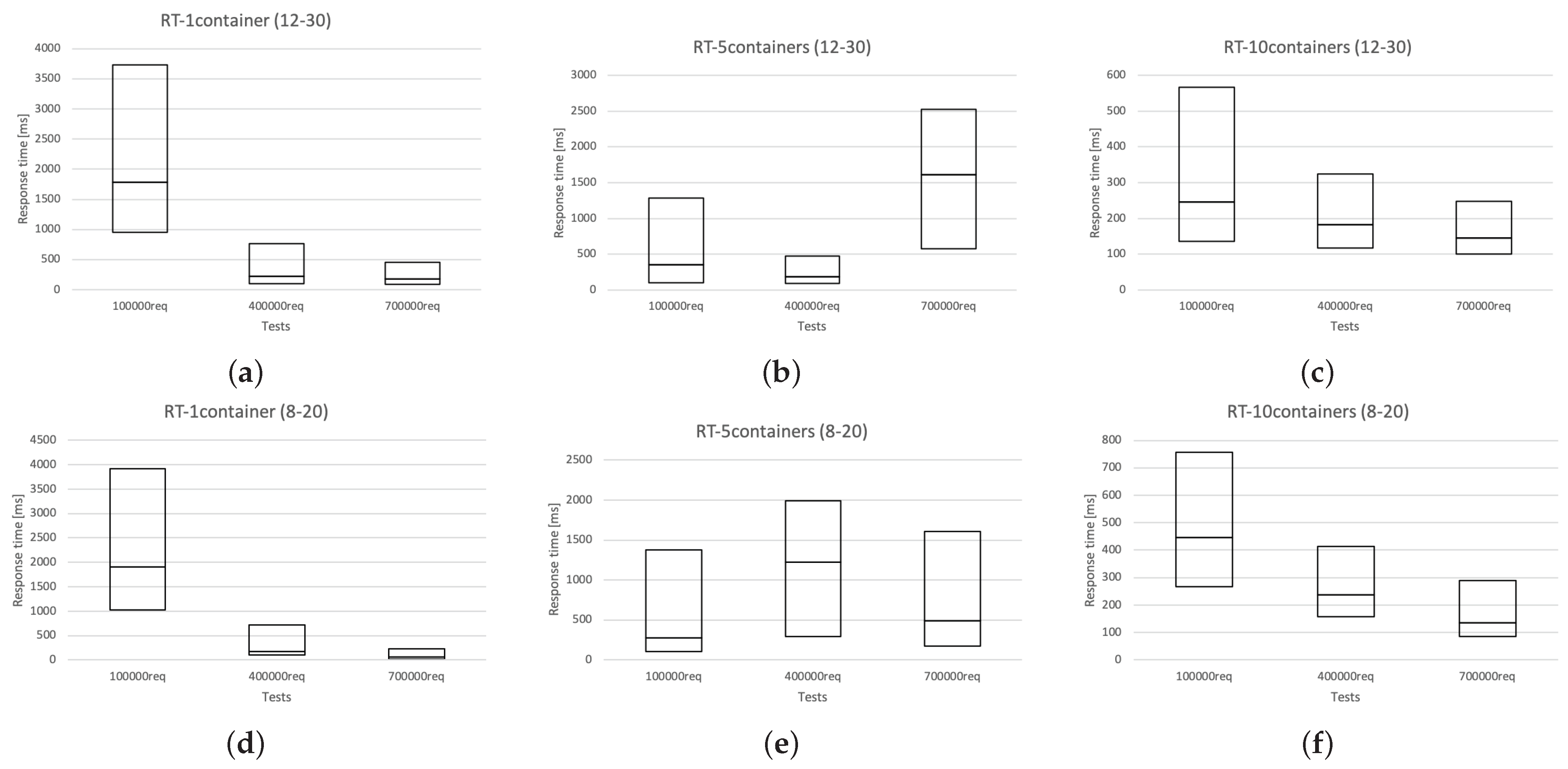
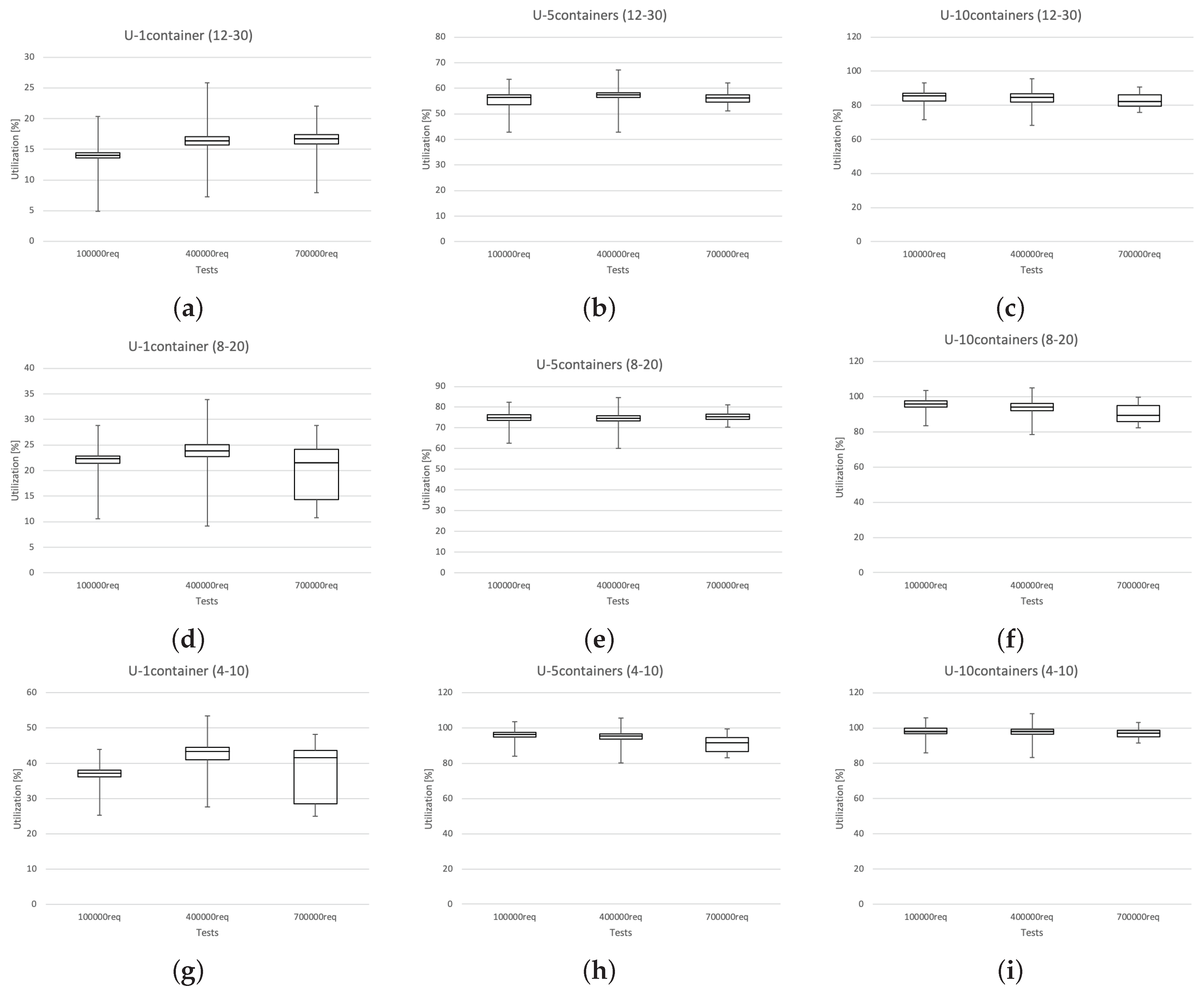
3.5. Experiment Results

Finally, we describe the conducted experiments ($ET1-ET9$) in detail and present the results obtained from them. During the experiments, we monitored each container as well as every request. The monitoring process consists of two metrics: response time and utilization.

The example monitoring logs for 100,000 requests are depicted in figures (Figure 3 and Figure 4). These results are divided into two parts: the first part shows the response time (Figure 3) and the second shows the utilization (Figure 4) for each approach.

A stacked boxplot chart for response times is presented in figure (Figure 5 (Boxplots may also have lines (whiskers), but in this case, they were removed so as not to hinder the analysis.)).

A stacked boxplot chart for resource utilization (Figure 6). The CPU utilization is limited to 100% When the system utilization has values (bigger than 99%) close to that boundary ($ET8$ Figure 6h and $ET9$ Figure 6i), we have a problem with future estimations. The different architectures had similar workloads in particular cases, and load levels should be lower than 100%. In some cases, we could solve the issue of performance evaluation overloaded web server using a simulation-based approach [38]. The response time values of the tests $ET7-ET9$ ($Exp.3$) should not be taken into consideration in the estimations. We checked this in the following sections.

Direct measurement of resource demands may not be possible in some scenarios. Hence, we might estimate the resource demand based on the response time and CPU utilization metrics. Each measurement trace captures only one metric, and each trace corresponds to a specific container. The first trace contains a set $D_{RT}=\{\{t_1,r{t}_1\},\{t_2,r{t}_2\},...,\{t_m,r{t}_m\}\}$, where $t_i$ is a timestamp and $r{t}_i$ is the response time made at time $t_i$. The second trace contains a set $D_U=\{\{t_1,u_1\},\{t_2,u_2\},...,\{t_n,u_n\}\}$, where $t_j$ is a timestamp with an interval of 30 s and $u_j$ is average CPU utilization in time interval $t_j-t_{j-1}$. The following section presents statistical methods that use monitoring datasets to estimate resource demands.

4. Resource Demand Prediction

This section elaborates on the approach used for estimating resource demand. Resource demand refers to the average time that a request takes to receive service from a resource (CPU) in a system, and the total number of visits to the resource, excluding waiting times. Measuring resource demand accurately with existing monitoring tools is challenging.

Numerous approaches for predicting resource demand have been proposed [16]. The precision of these predictions is significantly affected by the accuracy of the measurements. In our study, we used SEWS to analyse the response time and CPU utilization with realistic workloads generated by SELG. We measured all parameter values of SEWS using SELG and system tools while the system was running. Based on these values, we estimated the resource demand for each resource and one workload class. The estimation process uses data from container monitoring logs. However, the obtained values may differ from those obtained in native systems [5] since Docker containers are runtime instances of the corresponding images.

In this study, the estimation process is crucial, and its accuracy depends on the monitored traces. We executed the estimation process on the prepared monitoring data, which consists of a set of measurements (output parameters) obtained by the SEWS benchmark.

4.1. Estimation Parameters

Our attention is directed towards statistical methods for predicting resource demand. To forecast resource demand, we require two real production system parameters: request response time and resource utilization. Response time is dependent on resource demand, residence time, and workload intensity. For a specific resource, response time is the sum of the residence times, which includes queuing time and resource demand [5].

4.2. Approaches to Resource Demand Prediction

Mathematical methods commonly used for resource demand estimation are presented on [16]. Based on https://se.informatik.uni-wuerzburg.de/software-engineering-group/tools/librede/ (accessed on 31 August 2023) LibReDE we ensured representative methods for evaluation. The interpretation of the results involves identifying the magnitude of errors associated with measurement anomalies for each of the methods, with the method having the smallest error considered as the best estimate.

4.3. LibReDE Estimates

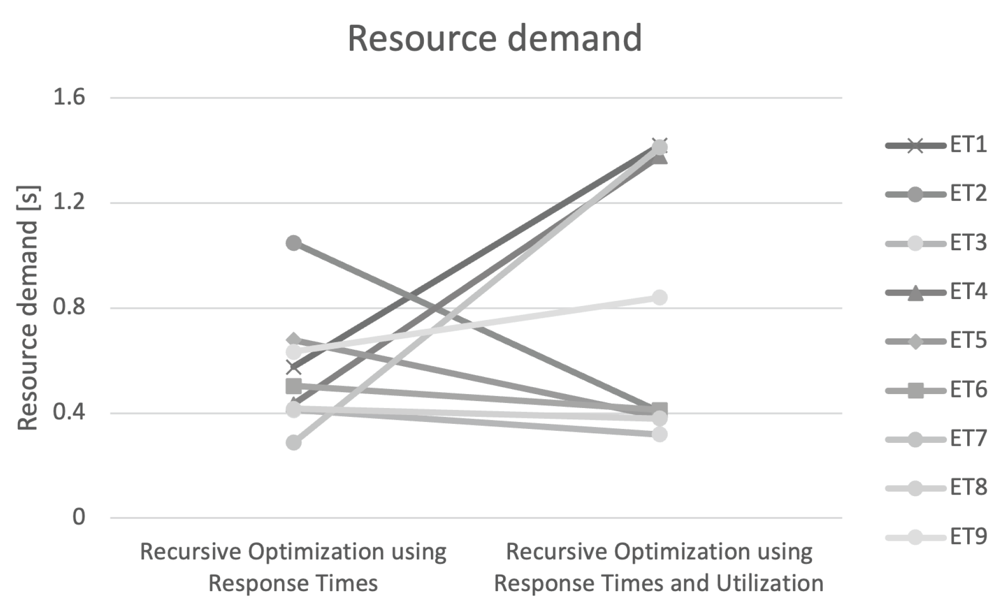
In this subsection, our aim is to evaluate the accuracy of different resource demand estimation approaches in our environment. To achieve this, we utilized the Library for Resource Demand Estimation (LibReDE) developed by Spinner et al. [16], which is used for offline analysis.

LibReDE currently supports implementations of the following estimation methods: (1) approximation with response time, (2) Kalman filter using response time and utilization, (3) Kalman filter using utilization law, (4) least-squares regression using queue lengths and response time, (5) least-squares regression using utilization law, (6) recursive optimization using response time (RORT), (7) recursive optimization using response time and utilization (RORTU), (8) service demand law. This tool calculates the estimated validation error using the estimated relative response time error and the estimated relative utilization error [16]. Therefore, first, we concentrated on the estimation of the resource demand error.

Table 5. The quality of proposed estimation methods (1–8) for each test.

	1	2	3	4
$ET1$	−33.73121568	19.84842247	845.240542	−95.91645773
$ET2$	−6487.021564	946.457702	42,268.09643	38.10226782
$ET3$	0.379664096	0.370576906	357,284 224.4	0.388762798
$ET4$	−0.070396545	−1.235334562	1 130.442687	0.113804428
$ET5$	37 399.04116	120.538286	27 120.31354	−459.1572704
$ET6$	0.400369085	0.383722564	167 698.4815	0.409635151
$ET7$	1.450755404	1.363932945	831.2420911	1.486306432
$ET8$	−3.776294824	98.19939577	42 774.64724	−2.776643656
$ET9$	30.65167827	4.205167963	99 186.91791	16.31688764
	5	6	7	8
$ET1$	729.2034814	0.646818098	−0.897905511	845.2399791
$ET2$	33 164.44074	79.38060097	0.430180122	44 323.6072
$ET3$	356 184 355.5	0.351120179	0.230979692	356 208 326.1
$ET4$	1 124.470638	0.771952155	1.04651969	1,130.443295
$ET5$	23 732.13498	3.154876279	−322.1905826	27,191.73684
$ET6$	143,759.0219	0.394169807	0.355737927	170 410.6652
$ET7$	826.9900691	1.899608047	1.891813012	831.2422076
$ET8$	35,480.82464	7.169014737	0.323881793	42 784.55392
$ET9$	96,552.10109	0.669395411	1.977049405	99,190.83672

shows the estimation error for every estimation method (1–8) and tests ($ET1-ET9$).

Most methods show a significant accuracy loss, and we are seeking an approach that yields the most precise resource demand estimates. To achieve this, we selected the approaches with the lowest relative error by summing the relative utilization error with the relative response time error and choosing the approaches with the minimum total error. Our analysis, as shown in table (Table 5), indicates that RORT and RORTU have relatively small errors compared to other methods. After conducting multiple validation methods, we selected the two methods (numbers 6 and 7) with the least error.

Resource demand for the CPUs of the backend containers was estimated as they were identified in [1] as potential bottlenecks under heavy workload. The performance model did not consider other resources.

The consideration only focuses on two selected methods within LibReDE (Figure 7). These two estimation techniques (RORT and RORTU) are based on recursive optimization [39].

4.4. Results

In conclusion, we will present the findings of our resource demand estimation and determine the most appropriate estimation approach. The measurement data were obtained from our experiments as described in Section 3.5, and we utilized these data to make our estimates in Section 4.3. Resource demand is a concept derived from queuing theory, representing the time a request spends using a resource. As resource demands are random variables, we reported the mean values.

Now, we combined the two values of estimation RORT [40] and RORTU [41], and computed the average value as a result. The final estimated resource demand is depicted in the table. Table (

Table 6. Average resource demand for each test.

	$\mathit{Resource}\_\mathit{Demand}$ [s]	$1/\mathit{Resource}\_\mathit{Demand}$ [req/s]
$ET1$	0.997588333	1.002417497
$ET2$  ${}^{(}$${}^a$${}^{)}$	0.727264667	1.37501524
$ET3$  ${}^{(}$${}^a$${}^{)}$	0.3652765	2.737652162
$ET4$	0.905941667	1.10382383
$ET5$  ${}^{(}$${}^a$${}^{)}$	0.532029333	1.879595611
$ET6$  ${}^{(}$${}^a$${}^{)}$	0.457546	2.185572598
$ET7$	0.849838333	1.176694391
$ET8$  ${}^{(}$${}^a$${}^{)}$	0.397753	2.514123086
$ET9$  ${}^{(}$${}^a$${}^{)}$	0.736487259	1.35779674

${}^{(}$${}^a$${}^{)}$ Values for a single container.

) shows the average resource demand and throughput X for the container [20]. Estimation results for tests ($ET8$ and $ET9$) were crossed out and finally rejected due to the verification of the simulations presented in Section 5.

The QPN model is parameterised using the estimated resource demand values.

5. QPN Simulations

Before the model simulation, various parameters need to be quantified. The parameters of the PMs are:

• Number of requests;
• Number of requests per second;
• Kind of resources;
• Request classes;
• Resource demands;
• Scenarios of requests with route probability.

Usually, test experiments $Exp.1-Exp.3$ (Section 3) on the system under study are required to obtain these data. We designed a few different simulations $Sim.1-Sim.3$ to validate the accuracy of our approach. Now, we can use the estimated resource demands in the simulation models ($QPN1$, $QPN5$, and $QPN10$).

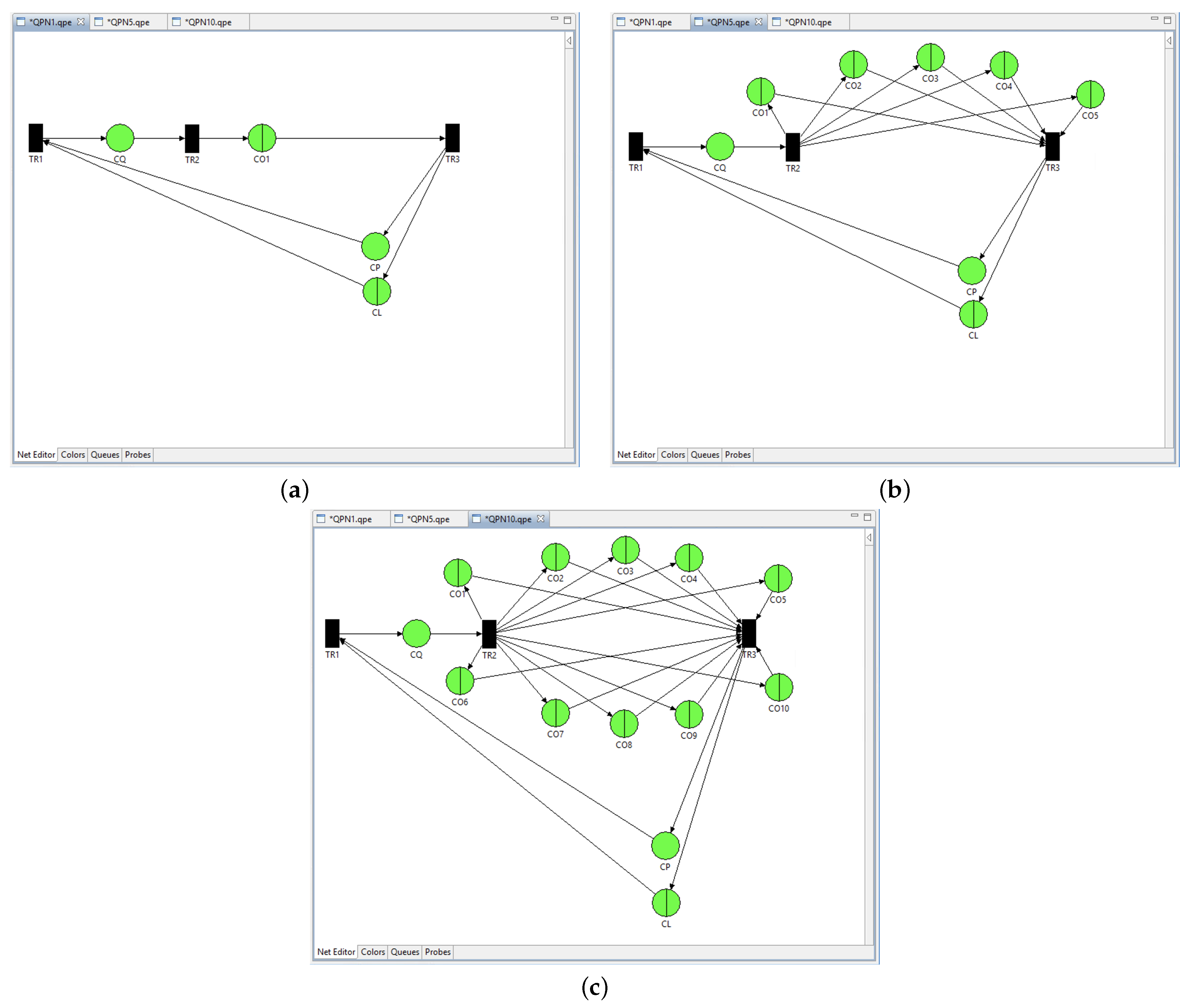
5.1. Queueing Petri Nets

At a high level, the systems could be modelled as a single queueing system. If a more detailed model is required, all devices are modelled as specific queueing systems. The performance model needs to consider the performance conditions of a container-based system.

We used a queueing simulator with $M/M/1$ queue and an open workload that logs the statistics of each request. We use the QPN modeling formalism [42] for our performance model. Figure 8 illustrates the QPN model of the SEWS. QPN models play a powerful role in the study of web systems [1,28]. It consists of a $CL$ queueing place and $CO1-10$ queueing places for every Docker backend container. The client queueing place $CL$ includes an Infinite Server scheduling queue and Docker backend containers queueing places $CO1-10$ include a first in–first out queue. All queues have an exponential service time distribution. The mean service time of $CL$ queue is equal to the thinking time configured in the load generator (SELG) for a particular test. $CL$ contains an initial token population of the client corresponding to the configured number of users in the SELG. Transition $TR1$ includes one mode. This mode consumes the token colour of clients and produces one token colour with the value. One token colour is defined in the container places for one workload class. The mean service time is set to the estimated resource demand of one workload class based on a particular test on the SELG. The transition $TR2$ takes a token from place $CQ$ and puts it into queueing places $CO1-10$. Place $CQ$ contains a colour definition for one workload class. The service times are set to the estimated resource demands of the backend server (SEWS). Finally, transition $TR3$ consumes a token and puts a token colour of a client in place $CL$.

To analyse the QPN model, we would use the discrete event simulator https://se.informatik.uni-wuerzburg.de/software-engineering-group/tools/qpme/ (accessed on 31 August 2023) [13], which can measure the response time of individual tokens in several places. We create a performance model of our system and parameterise it into, among other parameters, the resource demand parameter.

Input Parameters

In this subsection, we will describe the specific model configurations that we applied for the presented comparison. The values of input parameters for simulation tests ($ST1-ST9$) need to be known before simulation (

Table 7. Input parameters of simulation 1 (client and system).

Parameter	$\mathit{Sim}.1$
Number of servers ${}^{(}$${}^a$${}^{)}$	12
QPNi model ${}^{(}$${}^b$${}^{)}$	1	5	10
SimulationTest	$ST1$	$ST2$	$ST3$
$CL$ queueing place	90
$X_{CL}$ – [req/s]	6.242	4.849	3.826
$CP$ place ${}^{(}$${}^c$${}^{)}$	90
$X_{CO}$ – [req/s]	1.002	1.375	2.737

${}^{(}$${}^a$${}^{)}$ First in–first out scheduling strategy. ${}^{(}$${}^b$${}^{)}$i—QPN models ($QPN1$, $QPN5$, $QPN10$) for different number of containers (1, 5, 10). ${}^{(}$${}^c$${}^{)}$ Connection for containers—initial marking.

,

Table 8. Input parameters of simulation 2 (client and system).

Parameter	$\mathit{Sim}.2$
Number of servers ${}^{(}$${}^a$${}^{)}$	12
QPNi model ${}^{(}$${}^b$${}^{)}$	1	5	10
SimulationTest	$ST4$	$ST5$	$ST6$
$CL$ queueing place	90
$X_{CL}$ – [req/s]	6.732	5.064	2.975
$CP$ place ${}^{(}$${}^c$${}^{)}$	90
$X_{CO}$ – [req/s]	1.103	1.879	2.185

${}^{(}$${}^a$${}^{)}$ First in–first out scheduling strategy. ${}^{(}$${}^b$${}^{)}$i—QPN models ($QPN1$, $QPN5$, $QPN10$) for different number of containers (1, 5, 10). ${}^{(}$${}^c$${}^{)}$ Connection for containers—initial marking.

and

Table 9. Input parameters of simulation 3 (client and system).

Parameter	$\mathit{Sim}.3$
Number of servers ${}^{(}$${}^a$${}^{)}$	12
QPNi model ${}^{(}$${}^b$${}^{)}$	1	5	10
SimulationTest	$ST7$	$ST8$	$ST9$
$CL$ queueing place	90
$X_{CL}$ – [req/s]	6.366	3.152	1.644
$CP$ place ${}^{(}$${}^c$${}^{)}$	90
$X_{CO}$ – [req/s]	0.164	0.317	0.610

${}^{(}$${}^a$${}^{)}$ First in–first out scheduling strategy. ${}^{(}$${}^b$${}^{)}$i—QPN models ($QPN1$, $QPN5$, $QPN10$) for different number of containers (1, 5, 10). ${}^{(}$${}^c$${}^{)}$ Connection for containers—initial marking.

)). The measured customer throughput $X_{CL}$ at SELG in each test was taken into account and calculated container average throughput $X_{CO}$ on the basis of the estimated resource demands were included.

5.2. Results and Errors of Simulations

In this section, we present the results of the simulations and discuss our findings, with a focus on response time. To ensure consistency, each model simulated the same number of requests with exponential inter-arrival times and resource demands. We repeated each simulation for a specific number of requests (100,000, 400,000, and 700,000), resulting in different traces. For each set of test traces $(D_{TR},D_U)$, we estimated the resource demand separately.

In the following, we will analyse table (

Table 10. Response time prediction error.

	$\mathit{ST}1$	$\mathit{ST}2$  ${}^{(}$${}^{\mathit{a}}$${}^{)}$	$\mathit{ST}3$  ${}^{(}$${}^{\mathit{a}}$${}^{)}$
Simulation [s]	1.003483	1.222707	0.528284
Measured [s]	0.904	1.014	0.599
Error [%]	−11.00475664	−20.58254438	11.80567613
	$ST4$	$ST5$  ${}^{(}$${}^a$${}^{)}$	$ST6$  ${}^{(}$${}^a$${}^{)}$
Simulation [s]	1.075831	0.832224	0.711255
Measured [s]	1.128	0.928	0.871
Error [%]	4.624911348	10.32068966	18.34041332
	$ST7$	$ST8$  ${}^{(}$${}^a$${}^{)}$	$ST9$  ${}^{(}$${}^a$${}^{)}$
Simulation [s]	0.851	1.914936	2.031159
Measured [s]	0.804	1.455	0.846
Error [%]	−5.845771144	−31.61072165	−140.0897163

${}^{(}$${}^a$${}^{)}$ The single container.

) for more details on the results. The goal of the analysis presented in this section is also to compare simulation ($ST1-ST9$) and experiment ($ET1-ET9$) response times. We compared the simulated response time with the real response time. Then, we could evaluate the accuracy of the simulation predictions obtained with the estimated resource demands. We analyse the performance model and compare the predicted average response time with measurements from the realistic system. Table (Table 10) depicts the development of the total mean relative error for particular cases. Results for the two last cases are not taken into account in further analysis. In these cases, the system was overloaded by clients. The error is already significant. Both the measurement (Section 3) and estimation (Section 4), and hence the simulations (Section 5), may be burdened with an error. That becomes visible when the response time values were compared. The main reason for the incorrect measurement is reaching the limit of 100% for CPU utilization in the tests ($ET8$ and $ET9$). We also conclude that optimization methods (from Section 4) in other cases (lower than 100% CPU utilization) provide reliable estimates of resource demand. The average relative error of this approach is very slight. In the simulations, an average response time relative error is below 20%. These simulation results are at an acceptable level and in line with the experimental results.

6. Conclusions

This paper introduces a quantitative approach to meet performance requirements for container-based web systems through resource demand estimation. Although our PE covers multi-container environments, our focus is on evaluating the performance of individual containers.

To facilitate performance prediction for container environments, we developed a response time analysis tool. Our study highlights the challenges of performance modelling in containerized environments and identifies several issues encountered when applying response time analysis approaches, including:

• Individual simulation approaches for different numbers of containers are required.
• The containerized platform causes additional delays.

In our research, we delved into the performance of a containerized SEWS application, leveraging server access logs from various workload scenarios. Through meticulous data collection, we implemented multiple methodologies to estimate resource demand, notably using the LibReDe tool. Our rigorous offline evaluation pinpointed the most effective method, which was further validated in a real-world container environment. Utilizing the QPME tool, grounded in QPN models, we conducted a response time simulation analysis, aligning it with our resource demand estimates. Subsequent comparative experiments between our benchmarks and a queueing system simulator highlighted discrepancies in predicted response times, with errors ranging between 5 and 20%. Nevertheless, our innovative methodology offers a robust framework for developing container-based web systems, reinforcing insights from prior research on native systems [16] and underscoring the potential for performance evaluation in container-centric architectures.

The findings of this research hold significant physical implications for the realm of container-based web systems. By introducing a quantitative methodology, this study addresses the pressing need for performance optimization in such systems. The development of a response time analysis tool not only aids in predicting performance but also underscores the inherent challenges of modelling in containerized environments. For instance, the necessity for distinct simulation strategies based on the number of containers and the inherent delays introduced by the containerized platform are crucial insights. Through an in-depth analysis of a containerized SEWS application, the study bridges the gap between theoretical modelling and real-world application, using server access logs to gauge performance under varying workload scenarios. The rigorous evaluation process, which juxtaposed the accuracy of estimations from a production system against a queueing system simulator, revealed a modest error margin in predicted response times. This not only validates the methodology but also offers a blueprint for designing efficient container-based web systems. Furthermore, the alignment of these results with prior research on native systems reinforces the reliability and applicability of the findings. As industries increasingly adopt container-based systems, the insights from this study will be pivotal in guiding performance optimization strategies, paving the way for more efficient and responsive web applications.

The work presented in this study suggests multiple avenues for future research. It should be noted that the conceptual contribution of this study is not affected by considering only one request class and scenario. However, in future research, the estimation of resource demands for multiple request classes should be explored to make the model more realistic. Future research avenues, such as the exploration of resource demands for diverse request classes, promise to further refine and enhance the model’s realism and applicability.

References

1. Rak, T. Formal Techniques for Simulations of Distributed Web System Models. In Cognitive Informatics and Soft Computing; Springer: Singapore, 2021; pp. 365–380. [Google Scholar] [CrossRef]
2. Xia, B.; Li, T.; Zhou, Q.; Li, Q.; Zhang, H. An Effective Classification-Based Framework for Predicting Cloud Capacity Demand in Cloud Services. IEEE Trans. Serv. Comput. 2021, 14, 944–956. [Google Scholar] [CrossRef]
3. Chen, D.; Zhang, X.; Wang, L.; Han, Z. Prediction of Cloud Resources Demand Based on Hierarchical Pythagorean Fuzzy Deep Neural Network. IEEE Trans. Serv. Comput. 2021, 14, 1890–1901. [Google Scholar] [CrossRef]
4. Rak, T.; Żyła, R. Using Data Mining Techniques for Detecting Dependencies in the Outcoming Data of a Web-Based System. Appl. Sci. 2022, 12, 6115. [Google Scholar] [CrossRef]
5. Rak, T. Performance Modeling Using Queueing Petri Nets. In Computer Networks, Proceedings of the 24th International Conference on Computer Networks, Ladek Zdroj, Poland, 20–23 June 2017; Communications in Computer and Information Science; Springer International Publishing: Berlin/Heidelberg, Germany, 2017; Volume 718, pp. 321–335. [Google Scholar] [CrossRef]
6. Cherbal, S. Load balancing mechanism using mobile agents. Informatica 2021, 45, 257–266. [Google Scholar] [CrossRef]
7. Nguyen, V.Q.; Nguyen, V.H.; Nguyen, M.Q.; Huynh, Q.T.; Kim, K. Efficiently Estimating Joining Cost of Subqueries in Regular Path Queries. Electronics 2021, 10, 990. [Google Scholar] [CrossRef]
8. Zatwarnicki, K.; Zatwarnicka, A. Two-Layer Cloud-Based Web System. In Information Systems Architecture and Technology: Proceedings of 39th International Conference on Information Systems Architecture and Technology, San Francisco, CA, USA, 13–16 December 2018; Borzemski, L., Światek, J., Wilimowska, Z., Eds.; Springer: Cham, Switzerland, 2019; pp. 125–134. [Google Scholar] [CrossRef]
9. Pant, A. Design and Investigation of a Web Application Environment With Bounded Response Time. Int. J. Latest Trends Eng. Technol. 2019, 14, 31–33. [Google Scholar] [CrossRef]
10. Eismann, S.; Grohmann, J.; Walter, J.; von Kistowski, J.; Kounev, S. Integrating Statistical Response Time Models in Architectural Performance Models. In Proceedings of the 2019 IEEE International Conference on Software Architecture, Hamburg, Germany, 25–26 March 2019; pp. 71–80. [Google Scholar] [CrossRef]
11. Zhou, J.; Reniers, G. Modeling and analysis of vapour cloud explosions knock-on events by using a Petri-net approach. Saf. Sci. 2018, 108, 188–195. [Google Scholar] [CrossRef]
12. Giebas, D.; Wojszczyk, R. Atomicity Violation in Multithreaded Applications and Its Detection in Static Code Analysis Process. Appl. Sci. 2020, 10, 8005. [Google Scholar] [CrossRef]
13. Kounev, S.; Lange, K.D.; von Kistowski, J. Systems Benchmarking: For Scientists and Engineers; Springer: Berlin/Heidelberg, Germany, 2020. [Google Scholar] [CrossRef]
14. Walid, B.; Kloul, L. Formal Models for Safety and Performance Analysis of a Data Center System. Reliab. Eng. Syst. Saf. 2019, 193, 106643. [Google Scholar] [CrossRef]
15. Krajewska, A. Performance Modeling of Database Systems: A Survey. J. Telecommun. Inf. Technol. 2019, 8, 37–45. [Google Scholar] [CrossRef]
16. Spinner, S.; Walter, J.; Kounev, S. A Reference Architecture for Online Performance Model Extraction in Virtualized Environments. In Proceedings of the Companion Publication for ACM/SPEC on International Conference on Performance Engineering, New York, NY, USA, 22–26 April 2016; pp. 57–62. [Google Scholar] [CrossRef]
17. Doc, V.; Nguyen, T.B.; Huynh Quyet, T. Formal Transformation from UML Sequence Diagrams to Queueing Petri Nets. In Advancing Technology Industrialization Through Intelligent Software Methodologies, Tools and Techniques; IOS Press: Clifton, VA, USA, 2019; pp. 588–601. [Google Scholar] [CrossRef]
18. Fiuk, M.; Czachórski, T. A Queueing Model and Performance Analysis of UPnP/HTTP Client Server Interactions in Networked Control Systems. In Computer Networks; Communications in Computer and Information Science; Springer International Publishing: Berlin/Heidelberg, Germany, 2019; pp. 366–386. [Google Scholar] [CrossRef]
19. Rzońca, D.; Rzasa, W.; Samolej, S. Consequences of the Form of Restrictions in Coloured Petri Net Models for Behaviour of Arrival Stream Generator Used in Performance Evaluation. In Computer Networks; Gaj, P., Sawicki, M., Suchacka, G., Kwiecień, A., Eds.; Springer: Cham, Switzerland, 2018; pp. 300–310. [Google Scholar] [CrossRef]
20. Rak, T. Cluster-Based Web System Models for Different Classes of Clients in QPN. In Communications in Computer and Information Science; Springer International Publishing: Cham, Switzerland, 2019; Volume 1039, pp. 347–365. [Google Scholar] [CrossRef]
21. Szpyrka, M.; Brzychczy, E.; Napieraj, A.; Korski, J.; Nalepa, G.J. Conformance Checking of a Longwall Shearer Operation Based on Low-Level Events. Energies 2020, 13, 6630. [Google Scholar] [CrossRef]
22. Requeno, J.; Merseguer, J.; Bernardi, S.; Perez-Palacin, D.; Giotis, G.; Papanikolaou, V. Quantitative Analysis of Apache Storm Applications: The NewsAsset Case Study. Inf. Syst. Front. 2019, 21, 67–85. [Google Scholar] [CrossRef]
23. Borzemski, L.; Kedras, M. Measured vs Perceived Web Performance. Adv. Intell. Syst. Comput. 2020, 1050, 285–301. [Google Scholar] [CrossRef]
24. Zatwarnicki, K. Providing Predictable Quality of Service in a Cloud-Based Web System. Appl. Sci. 2021, 11, 2896. [Google Scholar] [CrossRef]
25. Kosińska, J.; Zieliński, K. Autonomic Management Framework for Cloud-Native Applications. J. Grid Comput. 2020, 18, 779–796. [Google Scholar] [CrossRef]
26. Zatwarnicki, K.; Zatwarnicka, A. A Comparison of Request Distribution Strategies Used in One and Two Layer Architectures of Web Cloud Systems. In Computer Networs; Communications in Computer and Information Science; Springer International Publishing: Berlin/Heidelberg, Germany, 2019; pp. 178–190. [Google Scholar] [CrossRef]
27. Zatwarnicki, K.; Barton, S.; Mainka, D. Acquisition and Modeling of Website Parameters. In Advanced Information Networking and Applications, Proceedings of the 35th International Conference on Advanced Information Networking and Applications, Toronto, Canada, 12–15 May 2021; Lecture Notes in Networks and Systems; Barolli, L., Woungang, I., Enokido, T., Eds.; Springer: Berlin/Heidelberg, Germany, 2021; Volume 227, pp. 594–605. [Google Scholar] [CrossRef]
28. Herrnleben, S.; Grohmann, J.; Rygielski, P.; Lesch, V.; Krupitzer, C.; Kounev, S. A Simulation-Based Optimization Framework for Online Adaptation of Networks. In Simulation Tools and Techniques; Song, H., Jiang, D., Eds.; Springer: Cham, Switzerland, 2021; pp. 513–532. [Google Scholar] [CrossRef]
29. Rak, T. Modeling Web Client and System Behavior. Information 2020, 11, 337. [Google Scholar] [CrossRef]
30. Pawlik, R.; Werewka, J. Recreation of Containers for High Availability Architecture and Container-Based Applications. In Computer Networks, Proceedings of the 26th International Conference, CN 2019, Kamien Slaski, Poland, 25–27 June 2019; Volume 1039, pp. 287–298. [Google Scholar] [CrossRef]
31. Urbańczyk, W.; Werewka, J. Contribution Title Enterprise Architecture Approach to Resilience of Government Data Centre Infrastructure. In Information Systems Architecture and Technology, Proceedings of the 39th International Conference on Information Systems Architecture and Technology, San Francisco, CA, USA, 13–16 December 2018; Borzemski, L., Światek, J., Wilimowska, Z., Eds.; Springer: Cham, Switzerland, 2019; pp. 135–145. [Google Scholar] [CrossRef]
32. Suoniemi, S.; Meyer-Waarden, L.; Munzel, A.; Zablah, A.R.; Straub, D. Big data and firm performance: The roles of market-directed capabilities and business strategy. Inf. Manag. 2020, 57, 103365. [Google Scholar] [CrossRef]
33. Burgin, M.; Eberbach, E.; Mikkilineni, R. Processing Information in the Clouds. Proceedings 2020, 47, 25. [Google Scholar] [CrossRef]
34. Chen, X.; Guo, M.; Shangguan, W. Estimating the impact of cloud computing on firm performance: An empirical investigation of listed firms. Inf. Manag. 2022, 59, 103603. [Google Scholar] [CrossRef]
35. Zhu, B.; Guo, D.; Ren, L. Consumer preference analysis based on text comments and ratings: A multi-attribute decision-making perspective. Inf. Manag. 2022, 59, 103626. [Google Scholar] [CrossRef]
36. Neumann, A.; Laranjeiro, N.; Bernardino, J. An Analysis of Public REST Web Service APIs. IEEE Trans. Serv. Comput. 2021, 14, 957–970. [Google Scholar] [CrossRef]
37. Zhang, X.L.; Demirkan, H. Between online and offline markets: A structural estimation of consumer demand. Inf. Manag. 2021, 58, 103467. [Google Scholar] [CrossRef]
38. Suchacka, G.; Borzemski, L. Simulation-based performance study of e-commerce web server system-results for FIFO scheduling. Adv. Intell. Syst. Comput. 2013, 183, 249–259. [Google Scholar] [CrossRef]
39. Menascé, D.; Dowdy, L.; Almeida, V.A.F. Performance by Design—Computer Capacity Planning by Example; Prentice Hall Professional: Old Bridge, NJ, USA, 2004. [Google Scholar]
40. Menascé, D. Computing Missing Service Demand Parameters for Performance Models. In Proceedings of the International CMG Conference, Las Vegas, NV, USA, 7–12 December 2008; pp. 241–248. [Google Scholar]
41. Liu, Z.; Wynter, L.; Xia, C.; Zhang, F. Parameter inference of queueing models for IT systems using end-to-end measurements. Perform. Eval. 2004, 63, 36–60. [Google Scholar] [CrossRef]
42. Bause, F.; Buchholz, P.; Kemper, P. Hierarchically combined queueing Petri nets. In Proceedings of the International Conference on Analysis and Optimization of Systems Discrete Event Systems, Sophia-Antipolis, France, 15–17 June 1994; pp. 176–182. [Google Scholar] [CrossRef]
Figure 1. Methodology conceptual flowchart of all PE processes.
Applsci 13 09896 g001
Figure 2. Container system (horizontal scaling) with back-end: (a) one container C 1 , (b) five containers C 5 , and (c) ten containers C 10 .
Applsci 13 09896 g002
Figure 3. Measured response time—100,000 [req]: (a) E T 1 , (b) E T 2 , (c) E T 3 , (d) E T 4 , (e) E T 5 , (f) E T 6 , (g) E T 7 , (h) E T 8 , (i) E T 9 .
Applsci 13 09896 g003
Figure 4. Measured utilization—100,000 [req]: (a) E T 1 , (b) E T 2 , (c) E T 3 , (d) E T 4 , (e) E T 5 , (f) E T 6 , (g) E T 7 , (h) E T 8 , (i) E T 9 .
Applsci 13 09896 g004
Figure 5. Box plot of response time (without whiskers)—100,000, 400,000, 700,000 [req] with average value: (a) E T 1 —0.904 [s], (b) E T 2 —1.014 [s], (c) E T 3 —0.599 [s], (d) E T 4 —1.128 [s], (e) E T 5 —0.928 [s], (f) E T 6 —0.871 [s], (g) E T 7 —0.804 [s], (h) E T 8 —1.455 [s], (i) E T 9 —0.846 [s].
Applsci 13 09896 g005aApplsci 13 09896 g005b
Figure 6. Box plot of CPU utilization—100,000, 400,000, 700,000 [req] with average value: (a) E T 1 —15 [%], (b) E T 2 —54 [%], (c) E T 3 —81 [%], (d) E T 4 —22 [%], (e) E T 5 —72 [%], (f) E T 6 —90 [%], (g) E T 7 —39 [%], (h) E T 8 —93 [%], (i) E T 9 —97 [%].
Applsci 13 09896 g006
Figure 7. Resource demand for two estimation methods taken into account in the analysis.
Applsci 13 09896 g007
Figure 8. QPN nets: (a) Q P N 1 , (b) Q P N 5 , and (c) Q P N 10 .
Applsci 13 09896 g008