Abstract
There is a close relationship between the size and property of a reservoir and the production and capacity. Therefore, in the process of oil and gas field exploration and development, it is of great importance to study the macro distribution of oil–gas reservoirs, the inner structure, the distribution of reservoir parameters, and the dynamic variation of reservoir characteristics. A reservoir model is an important bridge between first-hand geologic data and other results such as ground stress models and fracture models, and the quality of the model can influence the evaluation of the sweet spots, the deployment of a horizontal well, and the optimization of the well network. Reservoir facies modeling and physical parameter modeling are the key points in reservoir characterization and modeling. Deep learning, as an artificial intelligence method, has been shown to be a powerful tool in many fields, such as data fusion, feature extraction, pattern recognition, and nonlinear fitting. Thus, deep learning can be used to characterize the reservoir features in 3D space. In recent years, there have been increasing attempts to apply deep learning in the oil and gas industry, and many scholars have made attempts in logging interpretation, seismic processing and interpretation, geological modeling, and petroleum engineering. Traditional training image construction methods have drawbacks such as low construction efficiency and limited types of sedimentary facies. For this purpose, some of the problems of the current reservoir facies modeling are solved in this paper. This study constructs a method that can quickly generate multiple types of sedimentary facies training images based on deep learning. Based on the features and merits of all kinds of deep learning methods, this paper makes some improvements and optimizations to the conventional reservoir facies modeling. The main outcomes of this thesis are as follows: (a) the construction of a training image library for reservoir facies modeling is realized. (b) the concept model of the typical sedimentary facies domain is used as a key constraint in the training image library. In order to construct a conditional convolutional adversarial network model, One-Hot and Distributed Representation is used to label the dataset. (c) The method is verified and tested with typical sedimentary facies types such as fluvial and delta. The results show that this method can generate six kinds of non-homogeneous and homogeneous training images that are almost identical to the target sedimentary facies in terms of generation quality. In terms of generating result formats, compared to the cDCGAN training image generation method, traditional methods took 31.5 and 9 times longer. In terms of generating result formats, cDCGAN can generate more formats than traditional methods. Furthermore, the method can store and rapidly generate the training image library of the typical sedimentary facies model of various types and styles in terms of generation efficiency.
1. Introduction
The continental sedimentary basin occupies a big part of the world’s exploration and development block, and it has the characteristics of multi-source, rapid phase change, and mixed sediment development. The nonhomogeneity of the reservoir is the main cause of the multi-solution and uncertainty in petroleum geology. Oil and gas exploration and development intelligence has been a hot topic. Many researchers have applied AI technology to logging, physical exploration, drilling and completion, reservoir engineering, CCUS, etc. [1,2,3,4,5,6,7,8,9,10,11]. However, there are still some problems, such as the small sample size, which cannot meet the requirements of deep learning, the difficulty of algorithm exploration, and application [12,13,14].
Starting from this century, the superiority of multi-point geostatistics is more and more obvious than the two-point geostatistics, which is based on variation. A lot of researchers have optimized the multi-point geostatistics algorithm, which has been used in many oil fields. Furthermore, the importance of training images as an important source of prior knowledge in multi-point geostatistics is becoming more and more obvious. Training images are one of the key factors to determine the effectiveness of simulation [15].
Training images are two- or three-dimensional data, which can be used to represent the structure of a target simulation model in multi-point geostatistics. Therefore, the training image includes nonhomogeneous geoid features, including geometry, connectivity, spatial distribution, and relation of the geoid [16]. Zhang further explains how important it is to build a training image library when using the multi-point geostatistical method. The training image is a quantitative representation of the a priori geological model. It is also proposed that constructing a multi-typed training image library will facilitate the advancement of multidirectional geostatistics based on this training image [17]. Zhang mainly explains the workflow and construction of training images in multi-point geostatistics [18]. More and more researchers pay attention to the acquisition of training images in multi-point geostatistics and their actual applications. It is believed that the acquisition of training images is a key factor in the success of multi-point geostatistics modeling [19]. Moreover, to satisfy the smooth hypothesis, it is necessary for the training image to have the following features: the pattern in the entire training image space must be uniformly distributed [20]; there must be repetitive patterns in the training pictures; and the structural characteristics of the sedimentary facies are not confined to a particular position in the training image, but are distributed across the entire training image grid, i.e., they do not need to be faithful to the well point constraints [21].
In recent years, there has been a lot of research on training images, which has led to a variety of methods to generate and evaluate images. The methods for constructing training images mainly include satellite images from modern deposition, theoretical deposition models for specific deposition systems [22,23,24,25], target-based simulation algorithms [26,27,28], and deposition process-based methods [29,30,31,32,33,34]. However, traditional training image construction methods have many disadvantages. Traditional methods using real-world data cannot reflect complex sedimentary facies types and have a single type, making them unsuitable for batch training image generation. Other methods require repeated calibration of simulation parameters, so practical application and modeling are still quite difficult. The traditional training image library is built for a particular type or even a particular reservoir.
In order to address the drawbacks of traditional methods, we implemented a method that can rapidly build up the training image library of several typical reservoirs. Establishing a reusable reservoir training image library is crucial for reservoir sedimentary facies modeling. This is of great significance for establishing accurate reservoir physical properties models. An accurate static geological model is the foundation for subsequent work steps. Therefore, this work is of great significance to numerical simulations, well network deployment, and reserve estimation.
In this paper, we propose to construct the training image library of typical reservoir sedimentary facies by means of deep learning.
In Section 1, we conduct an in-depth analysis of the important role of training images and training image libraries. The background on the existing methods for constructing training images and their limitations are provided. Finally, the purpose and significance of this study are clarified.
In Section 2, we provide a detailed implementation of the main method. Mainly including the construction of training datasets, labeling with a combination of One-Hot and Distributed Representation, and finally, the optimization of neural networks.
In the last three sections, the results of all tests in this study are presented and discussed. In addition, a summary of this study is provided.
2. Materials and Methods
As important prior knowledge, the training image library can be used to build the reservoir facies based on the training image. In this part, we analyze the thought and defect of the traditional training image library building approach, which is based on the traditional training image library. Then, we construct a training image library based on a conditional deep convolutional generation adversarial network (cDCGAN). This is the workflow for this section to clearly delineate the different steps and processes involved in constructing the training image library (Figure 1).
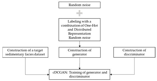
Figure 1.
Workflow for constructing the training image library.
2.1. Construction of a Typical Sedimentary Facies Training Dataset
2.1.1. Parameter Conditions
Traditional training image generation methods need to generate a special training image library according to the research goal. The constraint of the training image library is an important representation of a priori knowledge in the training images. In the traditional hand-drawn training image method, the geologist’s understanding of the sedimentary facies type in the study area is often used to distinguish the approximate size of the target body in combination with evidence of outcrop and modern sedimentation. In object-based training image generation, it is often necessary to restrict the target by using parameters such as the width, thickness, wavelength, amplitude of the target, and direction of the source (Table 1).

Table 1.
Description of training image parameter conditions.
In order to further accurately characterize the geometric morphology and spatial distribution characteristics of sedimentary facies, it is necessary to classify and qualitatively or even quantitatively describe this feature. First of all, it is mainly divided into the typical continental and marine-continental transitional sedimentary facies, i.e., it is common to differentiate the depositional types in different research areas. This is the basis for the classification of sedimentary facies types, as the sedimentary characteristics of different sedimentary types vary greatly. Secondly, we classify the facies in detail, taking the sedimentary subfacies and the sedimentary microfacies as the different sedimentary facies. Furthermore, the subfacies and depositional microfacies are shown as the primary object in the training image. Finally, the geometric parameters such as width, thickness, wavelength, amplitude, and source direction of the target body are used as an important constraint for the description of the sedimentary subfacies and the sedimentary microfacies. Therefore, a variety of training images are produced that can satisfy the requirements of facies modeling. The spatial distribution characteristics, trends, and erosion rules of geological bodies can characterize spatial variability. Geometric parameters can quantitatively characterize the geometric form of geological bodies. Thus, they are important for the description of sedimentary facies.
2.1.2. Training Image Generation of Typical Sedimentary Facies Using an Object-Based Method
In actual applications, it is necessary to select the type of training image in accordance with the expert’s knowledge of the regional geology. The selection of training images should be broadly representative of the type and distribution of regional sedimentary facies in order to provide a better understanding of the geology of the deep learning model. The training image set should include as many typical sedimentary systems as possible, and it can be easily constructed in batches. The training image results obtained from the target-based simulation method in PETREL® are used as the data for method testing, and a total of 60,000 braided river facies, straight river facies, meandering river facies, anastomosing river facies, braided river delta facies, and fan delta facies with a size of 100 × 100 were selected as the training images (Figure 2).
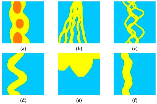
Figure 2.
Example of non-homogeneous and homogeneous training images: (a) braided river facies training image; (b) braided river delta facies training image; (c) anastomosing river facies training image; (d) meandering river facies training image; (e) fan delta facies training image; (f) straight river facies training image (yellow represents a river, fan or delta region, blue represents background).
2.2. cDCGAN
In this section, a convolutional generation adversarial neural network is used to train and learn the neural network using the typical reservoir sedimentary facies training images constructed in the previous section as the training data set and the typical reservoir sedimentary facies concept as the label data. On this basis, a deep learning approach is proposed to construct a typical reservoir training image library.
2.2.1. Structure of Neural Networks
Generative adversarial networks (GANs) are one of the representative models of generative networks. Since the disadvantage of GAN simulation is that it is too free, the output of GANs is not artificially controlled for larger pictures and complex data. Therefore, Mirza and Osindero proposed the theory of conditional generative adversarial networks by attaching constraint variables, such as class labels, to the original GANs [35].
2.2.2. One-Hot and Distributed Representation
- 1.
- One-Hot Representation
One of the most commonly used methods in NLP is One-Hot Representation, which uses a multi-bit state register to encode multiple states. In this method, word text is discretized and represented as a vector with only some non-zero dimensions, with each word using a different dimension. The characteristic of One-Hot Representation is that all words are independent. Clearly, this representation of the One-Hot Representation has a number of issues [36].
A word vector is a mathematical way used to represent human language, and the simplest vector approach is the One-Hot Representation form. For example, for the typical sedimentary facies in Table 2, the first element of 1 represents braided river facies, the fourth element of 1 represents anastomosing river facies, and the sixth element of 1 represents fan delta facies.
Table 2.
Example of One-Hot Representation.
In the One-Hot Representation, there is no semantic information, so it is impossible to express the difference of semantic association. For instance, the meaning of “Braided River Facies” is similar to that of “Meandering River Facies” and “Straight River Facies”. However, in this representation space, all word vectors are orthogonal. In this case, if the similarity of words is measured by cosine distance, then the similarity is 0. If Euclidean distance is used to measure the similarity of words, then all the words have the same meaning. The distances between words with similar meanings as well as unrelated words are the same. Moreover, to represent n words, it is necessary to set the length of a word expression to n, so that n words can be distinguished. This expression method loses the information related to the meaning between words. In particular, the vocabulary will increase exponentially when geometric parameters and information about the direction of the object source are added to the concept. The One-Hot Representation dimension will be increased accordingly, resulting in a dimensional catastrophe. As a result, One-Hot Representation is often confronted with the problems of exploding parameters and sparse data in practical applications.
- 2.
- Distributed Representation
Distributed Representation is an important tool in the field of deep learning, especially when it is used for natural language tasks. The concept of Distributed Representation was first used to represent concepts and is distinguished from One-Hot Representation. It is a novel approach to deal with dimensional disasters and local generalization constraints in machine learning and neural networks [37]. The Distributed Representation has many advantages over One-Hot Representation. The word vectors at this point are similar, as Table 3 shows.
Table 3.
Example of Distributed Representation.
Distributed Representation is a good way to overcome the problem of dimension disaster. Moreover, it is able to compute the similarity directly from the distance between two words. The reduction in the number of parameters is of great significance, since it not only reduces computation but also allows for a relatively few sample sizes to avoid overfitting [38].
- 3.
- Comparison between One-Hot and Distributed Representation
Figure 3 shows the two types of clustering. In the local representation (Figure 3a), each area is relatively independent, and a set of parameters is needed to characterize each area individually. In Distributed Representation (Figure 3b), different from the previous one, the parameters that describe the characteristics are shared, and each area can be characterized by a category representation 1–3. The ability of neural networks to learn distributed data representations is one of the main reasons why deep learning can be very effective for many different types of problems.
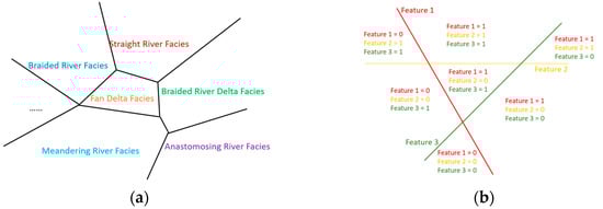
Figure 3.
Different representations of data samples (adapted from [38]): (a) One-Hot Representation; (b) Distributed Representation.
- 4.
- Labeling with a combination of One-Hot and Distributed Representation
Distributed Representation can be used to represent words with low dimensional density vectors, which can make it more difficult to differentiate between words. The One-Hot Representation has the advantages of simplicity, high efficiency, and better discrimination than Distributed Representation.
Based on these two representations, the training data set of neural networks are labeled as One-Hot Representation and Distributed Representation. Typical continental and continental transitional sedimentary facies are selected in the labeled data as the classification object of training image set. Moreover, the description terms of subfacies, deposition microfacies, and geometrical parameters are used to describe the main body of classification, which are an important label data.
In order to compare the different types of representations, the Curve River’s source direction and channel width are taken as an example to further explain One-Hot and Distributed Representation. As shown in Figure 4, the feature dimensions of One-Hot Representation will be increased. In the drawing, the four characteristics are: northwest target source wide channel, northwest target source narrow channel, northeast target source wide channel, and northeast target source narrow channel. Black circles indicate the activation state of a feature. This representation makes a good distinction between the categories, but it does not provide any information about the relationship between the training images.
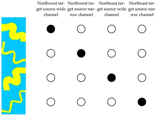
Figure 4.
One-Hot Representation of the training image (black circle represents the active state, white circle represents the inactive state, yellow represents a river region, blue represents background).
Figure 5 illustrates the Distributed Representation of the same training image. This approach is used to represent the information of the training image in relation to the concept of the source orientation and the channel width. The characteristic parameters include the northwest source, the northeast target source, the broad channel, and the narrow channel. The black circle indicates the activation status of a feature, and the characteristic parameters include the information of the training image and the relationship between different training images.
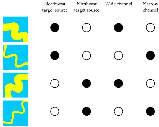
Figure 5.
Distributed Representation of the training image (black circle represents the active state, white circle represents the inactive state, yellow represents a river region, blue represents background).
No extra dimension is required when the Distributed Representation (for example, the training image in Figure 6) is used to represent a new training image. This is the true value of distributed representation: it is capable of finding “semantic similarity” among data by means of concepts.
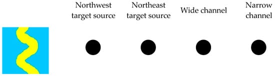
Figure 6.
Distributed Representation of a random implementation (black circle represents the active state, yellow represents a river region, blue represents background).
Based on the above analysis, One-Hot Representation can differentiate between different training images although it increases the dimension of the feature vector to some extent. Therefore, the training images of different deposition types are distinguished and labeled by this method. Distributed Representation is an effective way to build the relation between the training images with similar features. This correlation can also be expressed to form a new training image, as illustrated in Figure 6. Deep learning is one of the main reasons for the success of deep learning, which is based on deep neural networks. For this reason, the method uses the joint method of One-Hot Representation and Distributed Representation for labeling in Table 4.
Table 4.
Description of dataset annotation.
3. Application Effect
Different from the traditional GAN approach, cDGAN needs to input the sample tag data and the training set into the generator and discriminator simultaneously. The specific algorithm process is as follows:
The discriminator takes the image generated by the generator as input and identifies the output of the convolution layer as “false”. Then, the training image corresponding to the label information is fed into the convolution layer, and is finally judged as “true”. In this process, the identification ability of the discriminator is improved continuously.
Unlike GAN, cDGAN adds data labeled by a combination of One-Hot coding and distributed representation to the n-dimensional noise input to the generator. The image is obtained by inputting the random noise with the label information into the deconvolution layer. Then, an image produced by the generator is inputted to the discriminator, which is determined as “false”. The parameters of the discriminator are fixed, and the error is passed back to the generator. In this process, the discriminator and generator play each other, and finally produce a target that is similar to the training image. After the training of the two networks, the discriminator network is not able to distinguish the training image from the image produced by the generator network. Then the training process is finished. In this case, the generator network can produce an image similar to that of the training image.
In order to improve the performance of the neural network, a conditional convolutional neural network is proposed, which is based on the optimization strategy of neural networks. The key parameters of the network model are given in Table 5.
Table 5.
Description of neural network parameters.
3.1. Generation of Non-Homogeneous Training Images
On the basis of the training dataset in Section 2.1.2, 10,000 training images of braided river, braided river delta, and anastomosing river facies were generated.
In Figure 7, the training image generating result 1 and result 2 show two implementations of the training image for the non-homogeneous braided river facies. From 200 to 4400 steps, the sediment subfacies boundary becomes clear, and the flow is smooth. Meanwhile, the microfacies boundary of the channel bar became clear, and the different channels became independent from each other. After 4400 steps, the training image of the braided river facies is achieved, which is the same as the training image database.
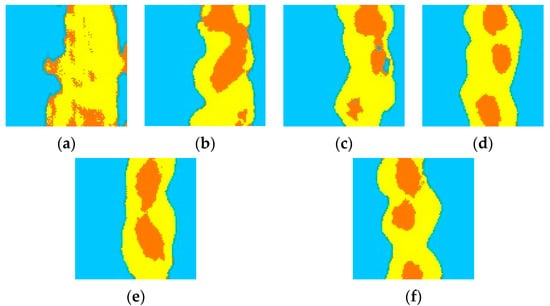
Figure 7.
Generation results of braided river facies training images: (a) 200 steps; (b) 2200 steps; (c) 4200 steps; (d) 6200 steps; (e) generation result 1; (f) generation result 2 (yellow represents a river region, blue represents background).
In Figure 8, the training image generating result 1 and result 2 illustrate two implementations of the training image for the non-homogeneous braided river delta facies. Between 200 and 5000 steps, the boundary between the river and the channel becomes clear, and the break of the river is improved with a smooth flow. Finally, after 5000 steps, it is possible to generate the training image of the braided river delta, which is the same as that in the training image library.
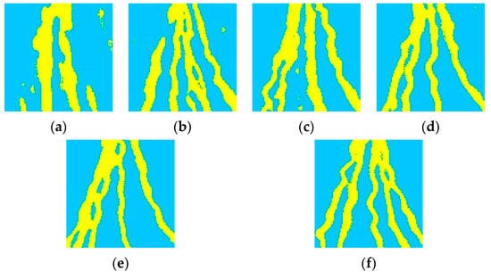
Figure 8.
Generation results of braided river delta facies training images: (a) 200 steps; (b) 2200 steps; (c) 4200 steps; (d) 6200 steps; (e) generation result 1; (f) generation result 2 (yellow represents a river region, blue represents background).
The training image generation result 1 and result 2 in Figure 9 show the two implementations of the training image for the non-homogeneous reticulated river facies. Between 200 and 5000 steps, the sediment subfacies boundary becomes distinct, the river continuity is strengthened, and the rivers are intercrossed in a clear network. After 5000 steps, it is basically possible to realize the generation of anastomosing river facies training images similar to those in the training image library.
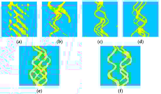
Figure 9.
Generation results of anastomosing river facies training images: (a) 200 steps; (b) 2200 steps; (c) 4200 steps; (d) 6200 steps; (e) generation result 1; (f) generation result 2 (yellow represents a river region, blue represents background).
3.2. Generation of Homogeneous Training Images
On the basis of the training dataset in Section 2.1.2, 10,000 uniform training images of fan delta facies, straight river facies, and meandering river facies are generated.
The training image generation result 1 and result 2 in Figure 10 show two implementations of the training image for the homogeneous fan delta facies. From 200 to 3200 steps, the boundary of divergent channel microfacies and interdivergent bay microfacies became clear, and the divergent channel microfacies spread out in a fan shape. After 3200 steps, it is possible to generate a fan delta facies training image similar to the one in the training image library.
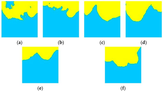
Figure 10.
Generation results of fan delta facies training images: (a) 200 steps; (b) 1200 steps; (c) 2200 steps; (d) 3200 steps; (e) generation result 1; (f) generation result 2 (yellow represents a river region, blue represents background).
The training image generation result 1 and result 2 in Figure 11 show two implementations of the training image for the homogeneous smooth river facies. From 200 to 2000 steps, the boundary of river sediment subfacies and flood bank subfacies is clarified, and the continuity of river is strengthened gradually. After 2000 steps, it is possible to generate the training image of the straight stream facies, which is the same as in the training image database. In Figure 12, the training image generating result 1 and result 2 show two implementations of the training image for the homogeneous meandering river facies. From 200–3200 steps, the sediment subfacies boundary becomes distinct, the river continuity is strengthened, and the width of the river becomes uniform. After 3200 steps, it is possible to generate the training image of the meandering stream, which is the same as that in the training image library.
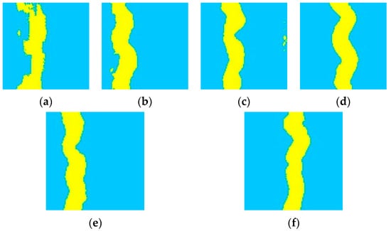
Figure 11.
Generation results of smooth river facies training images: (a) 200 steps; (b) 1200 steps; (c) 2200 steps; (d) 3200 steps; (e) generation result 1; (f) generation result 2 (yellow represents a river region, blue represents background).
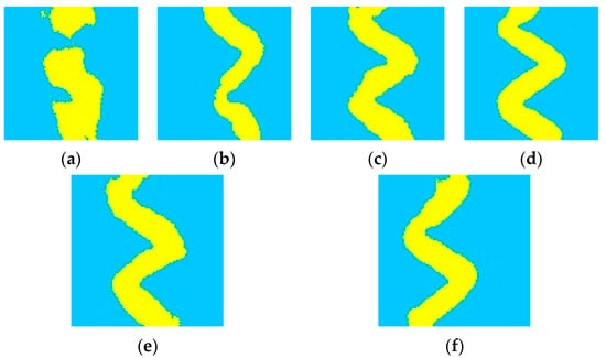
Figure 12.
Generation results of meandering river facies training images: (a) 200 steps; (b) 1200 steps; (c) 2200 steps; (d) 3200 steps; (e) generation result 1; (f) generation result 2 (yellow represents a river region, blue represents background).
3.3. Comparison between the Proposed cDCGAN-Based Approach and Traditional Methods for Training Image Library Construction
In order to elaborate on how this method addresses the limitations of traditional methods, we also compare the generation efficiency with traditional methods. The Facies Modeling function of Schlumberger’s Petrel modeling software can achieve various sedimentary facies modeling functions, among which Object-Based Facies Modeling can be combined with the workflow function to achieve target-based training image batch generation. Stanford University’s SGeMS modeling software can achieve simple modeling functions, with TIgenerator specifically used for batch generation of training images for multi-point geostatistics.
Overall, as shown in Figure 13, on the one hand, the cDCGAN-based training image generation approach is capable of producing a training image for a particular type of sedimentary facies in comparison with a conventional GAN-based unconditioned simulation. The cDCGAN-based approach, on the other hand, can produce a larger batch of training images, faster, and with more diversity than conventional training methods.
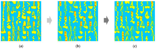
Figure 13.
Generation results of training images of multiple typical sedimentary facies: (a) 200 steps; (b) 3200 steps; (c) 5600 steps (yellow represents a river region, blue represents background).
Under the same calculation conditions, as shown in Table 6, with the goal of generating 1000 training images, Petrel, SGeMS, and cDCGAN took 634.6 s, 177.5 s, and 22.5 s, respectively. The average time to generate each training image was 0.63 s, 0.18 s, and 0.02 s, respectively. In terms of generating result formats, cDCGAN can generate formats that cover .GRDECL and .gslib, as well as image formats that can generate .jpg. In terms of the types of generated results, the first two training image generation methods can only meet the requirements of generating a single type of training image at a single time. With sufficient training, cDCGAN can quickly generate a variety of training image libraries based on the diversity of input labels, providing important support for reservoir facies modeling methods based on training images.
Table 6.
Comparison of commonly used training image generation methods.
4. Discussion
The combination of a deep learning and typical reservoir training image library construction method has a good application value for oil and gas field exploration and development. In order to combine the two methods organically, it is necessary to consider comprehensively the characteristics and properties of specific problems encountered in the process of constructing typical reservoir training image databases and the characteristics and advantages of deep learning methods. In the meantime, a great deal of practice should be conducted before this technique can achieve a good effect. In Section 3.1 and Section 3.2, case studies shows that cDCGAN can generate six kinds of different training images, which are almost the same as target sedimentary facies model. The dataset labeled with a combination of One-Hot and Distributed Representation (Section 2.2) make it possible to generate all of the six kinds of different training images at one time (results are shown in Section 3.3). In Section 3.3, the quality of the training images generated by this method can meet the requirements of reservoir facies modeling compared to traditional methods. In terms of generating result formats, compared to the cDCGAN training image generation method, traditional methods took 31.5 and 9 times longer. In terms of generating result formats, cDCGAN can generate more formats than traditional methods.
In the case of more sufficient data sources, more types of training images can also be generated. This proves the superior robustness of the method for constructing a training image library in this study. This article has generated training images for several main sedimentary types in the current research, which can also achieve the generation of more types of training images in terms of performance. During the process of this study, some challenges were indeed encountered. On the one hand, deep learning algorithms are still unfamiliar to geologists, so it will still take some time for the algorithms to be widely applied. On the other hand, obtaining a filed case of more types of sedimentary facies poses certain difficulties. However, more types of multiscale sedimentary facies still need to be included. Therefore, in the future, further attention should be paid to the production and generation of field case datasets. Adding more types of multi-scale sedimentary facies to the training set better reflects the advantages of this research method.
5. Conclusions
In order to realize a training image library construction method system for deep learning in typical multivariate geological data scenarios, this study solves the bottleneck of traditional training image libraries, and combines the advantages and disadvantages of various deep learning approaches. Aiming at the requirement of a reservoir facies modeling method based on training images for the training image database, which can store and quickly generate many typical deposition models, the flow of main research is as follows:
- An in-depth analysis is conducted on the urgent demand for training image libraries, and the disadvantages of traditional methods for constructing training image libraries are analyzed.
- A set of training images of typical sedimentary facies is generated by an object-based method, and the data annotation is carried out on the basis of One-Hot and Distributed Representation.
- Building cDCGAN to realize the construction of the training image database, which can store and quickly generate many typical sedimentary facies models.
- Taking the typical river facies and delta facies as an example, the method is validated and tested to realize the construction of a training image library based on deep learning for modeling typical reservoir facies, which provides important support for the establishment of a realistic reservoir model.
Author Contributions
Conceptualization, J.Y. and Y.L.; methodology, J.Y.; software, J.Y. and Y.L.; validation, J.Y., Y.L. and M.P.; investigation, J.Y., Y.L. and M.P.; resources, J.Y. and Y.L.; data curation, J.Y.; writing—original draft preparation, J.Y.; writing—review and editing, J.Y. and Y.L.; visualization, J.Y.; supervision. J.Y., Y.L. and M.P.; project administration, Y.L. and M.P.; funding acquisition, Y.L. All authors have read and agreed to the published version of the manuscript.
Funding
This research was funded by the following funds: 1. Project of R&D Department of Petrochina, grant No. 2021DJ2005 and No. 2202DJ8024. 2. Innovation fund of Petrochina, grant No. 2023-1433.
Institutional Review Board Statement
Not applicable.
Informed Consent Statement
Not applicable.
Data Availability Statement
All relevant data are within the manuscript.
Acknowledgments
The authors would like to thank the anonymous reviewers for the valuable comments.
Conflicts of Interest
The authors declare no conflict of interest.
References
- Iraji, S.; Soltanmohammadi, R.; Matheus, G.F.; Basso, M.; Vidal, A.C. Application of unsupervised learning and deep learning for rock type prediction and petrophysical characterization using multi-scale data. Geoenergy Sci. Eng. 2023, 230, 212241. [Google Scholar] [CrossRef]
- Zhang, L.H.; Kou, Z.H.; Wang, H.T.; Zhao, Y.L.; Dejam, M.; Guo, J.J.; Du, J. Performance analysis for a model of a multi-wing hydraulically fractured vertical well in a coalbed methane gas reservoir. J. Pet. Sci. Eng. 2018, 166, 104–120. [Google Scholar] [CrossRef]
- Liu, Y.; Zhang, X.; Guo, W.; Kang, L.; Yu, R.; Sun, Y. An Approach for Predicting the Effective Stress Field in Low-Permeability Reservoirs Based on Reservoir-Geomechanics Coupling. Processes 2022, 10, 633. [Google Scholar] [CrossRef]
- Ren, D.Z.; Wang, X.Z.; Kou, Z.H.; Wang, S.C.; Wang, H.; Wang, X.G.; Tang, Y.; Jiao, Z.S.; Zhou, D.S.; Zhang, R.J. Feasibility evaluation of CO2 EOR and storage in tight oil reservoirs: A demonstration project in the Ordos Basin. Fuel 2023, 331, 125652. [Google Scholar] [CrossRef]
- Fetisov, V.; Ilyushin, Y.V.; Vasiliev, G.G.; Leonovich, I.A.; Müller, J.; Riazi, M.; Mohammadi, A.H. Development of the automated temperature control system of the main gas pipeline. Sci. Rep. 2023, 13, 3092. [Google Scholar] [CrossRef] [PubMed]
- Liu, S.; Liu, Y.; Zhang, X.; Guo, W.; Kang, L.; Yu, R.; Sun, Y. Geological and Engineering Integrated Shale Gas Sweet Spots Evaluation Based on Fuzzy Comprehensive Evaluation Method: A Case Study of Z Shale Gas Field HB Block. Energies 2022, 15, 602. [Google Scholar] [CrossRef]
- Wang, H.T.; Kou, Z.H.; Guo, J.J.; Chen, Z.T. A semi-analytical model for the transient pressure behaviors of a multiple fractured well in a coal seam gas reservoir. J. Pet. Sci. Eng. 2021, 198, 108159. [Google Scholar] [CrossRef]
- Yao, J.; Liu, Q.; Liu, W.; Liu, Y.; Chen, X.; Pan, M. 3D Reservoir Geological Modeling Algorithm Based on a Deep Feedforward Neural Network: A Case Study of the Delta Reservoir of Upper Urho Formation in the X Area of Karamay, Xinjiang, China. Energies 2020, 13, 6699. [Google Scholar] [CrossRef]
- Pershin, I.M.; Papush, E.G.; Kukharova, T.V.; Utkin, V.A. Modeling of Distributed Control System for Network of Mineral Water Wells. Water 2023, 15, 2289. [Google Scholar] [CrossRef]
- Liu, Y.; Ma, X.; Zhang, X.; Guo, W.; Kang, L.; Yu, R.; Sun, Y. 3D geological model-based hydraulic fracturing parameters optimization using geology–engineering integration of a shale gas reservoir: A case study. Energy Rep. 2022, 8, 10048–10060. [Google Scholar] [CrossRef]
- Marinina, O.; Nechitailo, A.; Stroykov, G.; Tsvetkova, A.; Reshneva, E.; Turovskaya, L. Technical and Economic Assessment of Energy Efficiency of Electrification of Hydrocarbon Production Facilities in Underdeveloped Areas. Sustainability 2023, 15, 9614. [Google Scholar] [CrossRef]
- Kuang, L.C.; Liu, H.; Ren, Y.L.; Luo, K.; Shi, M.Y.; Su, J.; Li, X. Application and development trend of artificial intelligence in petroleum exploration and development. Pet. Explor. Dev. 2021, 48, 1–11. [Google Scholar] [CrossRef]
- Liu, Y.; Zhang, X.; Guo, W.; Kang, L.; Gao, J.; Yu, R.; Sun, Y.; Pan, M. Research Status of and Trends in 3D Geological Property Modeling Methods: A Review. Appl. Sci. 2022, 12, 5648. [Google Scholar] [CrossRef]
- Yao, J.; Liu, W.; Liu, Q.; Liu, Y.; Chen, X.; Pan, M. Optimized algorithm for multipoint geostatistical facies modeling based on a deep feedforward neural network. PLoS ONE 2021, 16, e0253174. [Google Scholar] [CrossRef]
- Wang, L.X.; Yin, Y.S.; Feng, W.J.; Duan, T.Z.; Zhao, L.; Zhang, W.B. A training image optimization method in multiple-point geostatistics and its application in geological modeling. Pet. Explor. Dev. 2019, 46, 703–709. [Google Scholar] [CrossRef]
- Journel, A.; Zhang, T. The necessity of a multiple-point prior model. Math. Geol. 2006, 38, 591–610. [Google Scholar] [CrossRef]
- Zhang, T. Incorporating geological conceptual models and interpretations into reservoir modeling using multiple-point geostatistics. Earth Sci. Front. 2008, 15, 26–35. [Google Scholar] [CrossRef]
- Zhang, T.; McCormick, D.; Hurley, N.; Signer, C. Applying multiple-point geostatistics to reservoir modeling—A practical perspective. In Proceedings of the EAGE Conference on Petroleum Geostatistics, Cascais, Portugal, 9–11 September 2007. [Google Scholar]
- Chen, H.Q.; Li, W.Q.; Hong, Y. Advances in Multiple-point Geostatistics Modeling. Geol. J. China Univ. 2018, 24, 593–603. [Google Scholar]
- Maharaja, A. TiGenerator: Object-based training image generator. Comput. Geosci. 2008, 34, 1753–1761. [Google Scholar] [CrossRef]
- Meerschman, E.; Pirot, G.; Mariethoz, G.; Straubhaar, J.; Meirvenne, M.V.; Renard, P. A practical guide to performing multiple-point statistical simulations with the Direct Sampling algorithm. Comput. Geosci. 2013, 52, 307–324. [Google Scholar] [CrossRef]
- Fadlelmula, M.; Killough, J.; Fraima, M. TiConverter: A training image converting tool for multiple-point geostatistics. Comput. Geosci. 2016, 96, 47–55. [Google Scholar] [CrossRef]
- Mitten, A.J.; Mullins, J.; Pringle, J.K.; Howell, J.; Clarke, S.M. Depositional conditioning of three dimensional training images: Improving the reproduction and representation of architectural elements in sand-dominated fluvial reservoir models. Mar. Pet. Geol. 2019, 113, 104156. [Google Scholar] [CrossRef]
- Iraji, S.; Soltanmohammadi, R.; Munoz, E.R.; Basso, M.; Vidal, A.C. Core scale investigation of fluid flow in the heterogeneous porous media based on X-ray computed tomography images: Upscaling and history matching approaches. Geoenergy Sci. Eng. 2023, 225, 211716. [Google Scholar] [CrossRef]
- Soltanmohammadi, R.; Iraji, S.; Almeida, T.R.; Basso, M.; Munoz, E.R.; Vidal, A.C. Investigation of pore geometry influence on fluid flow in heterogeneous porous media: A pore-scale study. Energy Geosci. 2024, 5, 100222. [Google Scholar] [CrossRef]
- Haldorsen, H.H.; Chang, D.M. Notes on stochastic shales: From outcrop to simulation model. In Reservoir Characterization; Academic Press: Cambridge, MA, USA, 1986; pp. 445–485. [Google Scholar]
- Deutsch, C.V.; Wang, L. Fluvsim: Hierarchical object-based stochastic modeling of fluvial reservoirs. Math. Geol. 1996, 28, 857–880. [Google Scholar] [CrossRef]
- Deutsch, C.V.; Tran, T.T. FLUVSIM: A program for object-based stochastic modeling of fluvial depositional systems. Comput. Geosci. 2002, 28, 525–535. [Google Scholar] [CrossRef]
- Ikeda, S.; Parker, G.; Sawai, K. Bend theory of river meanders. Part 1. Linear development. J. Fluid Mech. 1981, 112, 363–377. [Google Scholar] [CrossRef]
- Mariethoz, G.; Caers, J. Multiple-Point Geostatistics: Stochastic Modeling with Training Images; Wiley: Hoboken, NJ, USA, 2014. [Google Scholar]
- Koltermann, C.E.; Gorelick, S.M. Paleoclimatic signature in terrestrial flood deposits. Science 1992, 256, 1775–1782. [Google Scholar] [CrossRef] [PubMed]
- Pyrcz, M.J.; Boisvert, J.B.; Deutsch, C.V. ALLUVSIM: A program for event-based stochastic modeling of fluvial depositional systems. Comput. Geosci. 2009, 35, 1671–1685. [Google Scholar] [CrossRef]
- Hu, X.; Yin, Y.S.; Feng, W.J.; Wang, L.X.; Duan, T.Z.; Zhao, L.; Zhang, W.B. Establishment of training images of turbidity channels in deep waters and application of multi-point geostatistical modeling. Oil Gas Geol. 2019, 40, 1126–1134. [Google Scholar]
- Montero, J.M.; Colombera, L.; Yan, N.; Mountney, N.P. A workflow for modelling fluvial meander-belt successions: Combining forward stratigraphic modelling and multi-point geostatistics. J. Pet. Sci. Eng. 2021, 201, 108411. [Google Scholar] [CrossRef]
- Mirza, M.; Osindero, S. Conditional Generative Adversarial Nets. arXiv 2014, arXiv:1411.1784. [Google Scholar]
- Sun, F.; Guo, J.F.; Lan, Y.Y.; Xu, J.; Cheng, X.Q. A survey on distributed word representation. Chin. J. Comput. 2019, 42, 1605–1625. [Google Scholar]
- Hinton, G.E. Learning distributed representations of concepts. In Proceedings of the 8th Annual Conference of the Cognitive Science Society, Amherst, MA, USA, 15–17 August 1986. [Google Scholar]
- Sun, Z.J.; Xue, L.; Xu, Y.M.; Wang, Z. Overview of deep learning. Appl. Res. Comput. 2012, 29, 2806–2810. [Google Scholar]
Disclaimer/Publisher’s Note: The statements, opinions and data contained in all publications are solely those of the individual author(s) and contributor(s) and not of MDPI and/or the editor(s). MDPI and/or the editor(s) disclaim responsibility for any injury to people or property resulting from any ideas, methods, instructions or products referred to in the content. |
© 2023 by the authors. Licensee MDPI, Basel, Switzerland. This article is an open access article distributed under the terms and conditions of the Creative Commons Attribution (CC BY) license (https://creativecommons.org/licenses/by/4.0/).