Deep-Learning Multiscale Digital Holographic Intensity and Phase Reconstruction

Abstract

Addressing the issue of the simultaneous reconstruction of intensity and phase information in multiscale digital holography, an improved deep-learning model, Mimo-Net, is proposed. For holograms with uneven distribution of useful information, local feature extraction is performed to generate holograms of different scales, branch input training is used to realize multiscale feature learning, and feature information of different receptive fields is obtained. The up-sampling path outputs multiscale intensity and phase information simultaneously through dual channels. The experimental results show that compared to Y-Net, which is a network capable of reconstructing intensity and phase information simultaneously, Mimo-Net can perform intensity and phase reconstruction simultaneously on three different scales of holograms with only one training, improving reconstruction efficiency. The peak signal-to-noise ratio and structural similarity of the Mimo-Net reconstruction for three different scales of intensity and phase information are higher than those of the Y-Net reconstruction, improving the reconstruction performance.

1. Introduction

Digital holography is a technique that uses electronic components to record interference patterns (holograms) containing wavefront information of an observed object [1,2]. These holograms are then reconstructed into object representations using a computer called holographic reconstruction [3,4]. The computer simulates the diffraction of the hologram, generating the complex amplitude of the reconstructed object’s optical wave and acquiring both the intensity and phase information of the measured object. This process ultimately leads to the reconstruction of a three-dimensional image [5], called holographic reconstruction. However, traditional holographic reconstruction often faces challenges, including speckle noise, zero-order and conjugate images, and wrapped phase [6,7], making the reconstruction process complex and producing average image quality.

With the rapid development of computer software and hardware, deep-learning techniques have been widely applied in image processing [8], such as computational imaging [9], image segmentation [10], and super-resolution reconstruction [11]. Researchers have recently integrated deep-learning techniques into digital holography to address the problems encountered in traditional holographic reconstruction [12,13,14,15,16]. For example, Sinha et al. proposed using neural networks to achieve end-to-end coaxial digital holographic reconstruction [17]. Rivenson et al. used trained neural networks to eliminate the twin image artifacts in coaxial holographic reconstruction [18]. Wang et al. combined U-Net and Ozcan networks to propose eHoloNet, which can directly reconstruct holograms without considering the zero-order component [19]. Zhao et al. introduced Y-Net, a Y-shaped convolutional neural network, for off-axis hologram reconstruction. This network can simultaneously reconstruct intensity and phase information from a single input digital hologram [20]. The above-mentioned networks proposed by the researchers are based on a single-scale architecture, which is only able to handle input and output on a single scale. The acquisition of digital holograms requires a precise design of the experimental setup. The resulting holograms may have high-frequency information concentrated in one area and low-frequency information scattered around it, resulting in large hologram sizes and slow reconstruction speeds. Cropping only the high-frequency information for reconstruction may result in the loss of useful information from the surrounding regions, leading to lower reconstruction quality.

To address the above issues, we propose an enhanced deep-learning model called Mimo-Net. The model extracts locally important features from large-scale holograms in a small-scale form. It serially constructs three input branches within a single network structure, from global to local, to feed into the leading network. Mimo-Net enlarges the receptive field and obtains the global information and detail information under different receptive fields. It also uses a multiscale feature-extraction module to enhance feature extraction and improve reconstruction accuracy. Finally, the multiscale features can be input into a single down-sampling path. At the same time, the up-sampling path can simultaneously output intensity information and phase information of multiple scales in a dual-channel format.

2. Principles and Methods

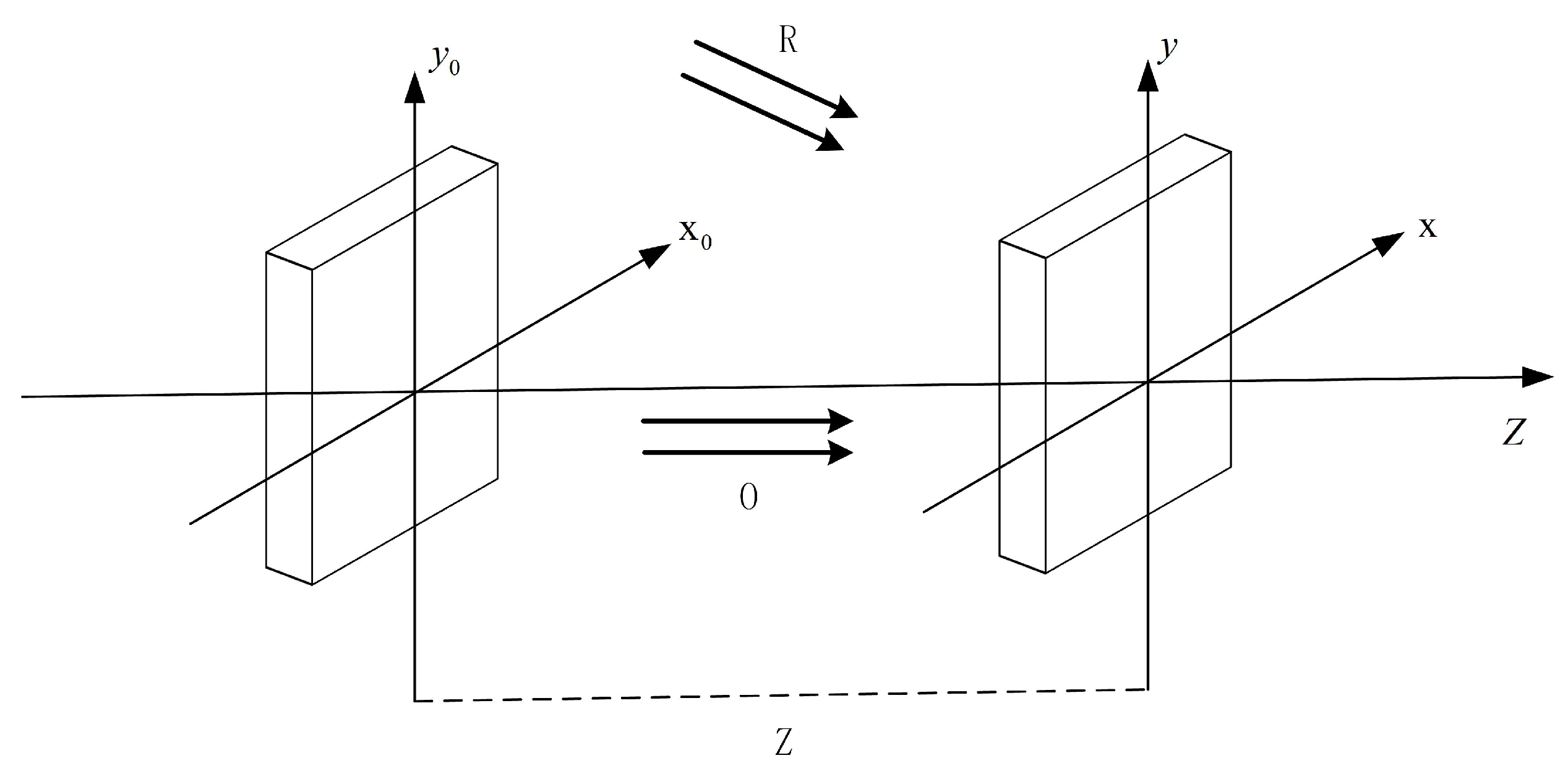
2.1. Principles of Digital Holography

Digital holography is a technique that uses the principle of interference to record and reconstruct the diffracted wavefront from an object as interference fringes [21,22]. A beam of light is split into two parts by a beam splitter. One part is the reference beam, which is directed to a photodetector, while the other is reflected from the object and serves as the object beam. These two beams interfere with each other, and the charge-coupled device (CCD) records the information from the interference fringes. This information contains the object beam’s intensity and phase information [23]. By reconstructing the hologram, the intensity and phase information of the object wave can be obtained [24,25].

The digital hologram system model is shown in Figure 1, where the $x_0$-$y_0$ plane is the object plane, the x-y plane is the hologram plane and Z is the recording distance. The off-axis holographic object wave interferes with the reference beam at a certain angle. The interference between R (reference beam) and O (object beam) on the plane results in the formation of a hologram. Let us assume that the complex amplitude distributions of the object and reference waves on the x-y plane are each represented by:

$$\begin{array}{c}O(x,y)=o(x,y)exp(-j\phi (x,y\left)\right),\hfill \end{array}$$

(1)

$$\begin{array}{c}R(x,y)=r(x,y)exp(-j\psi (x,y\left)\right),\hfill \end{array}$$

(2)

In the equation, $O^{*}(x,y)$ and $r^{*}(x,y)$ represent the intensity information of the object wave and reference wave, respectively, $\phi (x,y)$ and $\psi (x,y)$ represents the phase information of the object wave and reference wave, respectively. The recorded interference intensity at the image sensor level is Equation (3):

$$\begin{array}{c}I={\left|O(x,y)+R(x,y)\right|}^2\hfill \\ ={\left|O(x,y)\right|}^2+{\left|R(x,y)\right|}^2+2R(x,y)O(x,y)cos[\psi (x,y)-\phi (x,y)],\hfill \end{array}$$

(3)

The complex amplitude of the hologram can also be written in the following form of Equation (4):

$$\begin{array}{c}I={\left|O(x,y)\right|}^2+{\left|R(x,y)\right|}^2+O^{*}(x,y)R(x,y)+O(x,y)R^{*}(x,y),\hfill \end{array}$$

(4)

In the equation, $O^{*}(x,y)$ and $R^{*}(x,y)$ represent the conjugate terms of the complex amplitudes of the object wave and the reference wave, respectively. $|O(x,y){|}^2$ and $|R(x,y){|}^2$ on the right-hand side of the equation represent the intensity values of the object and reference waves, respectively: $O^{*}(x,y)R(x,y)$ represents the twin image, which is the conjugate field of the object wave; $O(x,y)R^{*}(x,y)$ represents the real image, corresponding to the field of the object wave. These four components together form the hologram of the measured object. Hologram reconstruction is the process of recovering intensity $o(x,y)$ and phase $\phi (x,y)$ from I.

2.2. Principles of Deep-Learning Reconstruction

Deep learning simulates the interference and diffraction of light in digital holography to establish the mapping relationship between holograms and intensity and phase information [26]. The process of interference between the reference beam and the object beam to form a hologram is regarded as the forward-propagation process of the digital holographic imaging system. For deep-learning networks, once the mapping function $R:I\to O$ is established, the reverse propagation for reconstruction from O to I can be completed. Therefore, the reconstruction process can be represented as:

$$\begin{array}{c}O(x,y)=P\left\{I\right(x,y\left)\right\},\hfill \end{array}$$

(5)

In Equation (5), P represents the mapping from the hologram to the object wavefront. In the network, P includes not only the process of removing conjugate images but also the process of diffraction propagation. Therefore, the objective function of the network model is:

$$\begin{array}{c}{\varphi }_0={arg}_{\varphi }min{\displaystyle \sum _{n=1}^N}L\left(O_n,P_{\varphi }\left\{I_n\right\}\right),\hfill \end{array}$$

(6)

In Equation (6), ${\varphi }_0^{}$ represents the optimal solution to the network weight parameters, L is the loss function, and N is the total number of training samples. In deep learning, the establishment of the mapping function is achieved through the process of fitting the data with a neural network $P_{\varphi }$ defined by the weight parameters $\varphi$, gradually obtaining a mapping model that closely approximates the true mapping function. The implementation steps of this process are usually as follows: first, obtaining many digital holograms along with their corresponding intensity and phase maps as the dataset, then constructing a neural network to fit this dataset. The network applies multi-layer convolutional operations to learn the image features of many intensity images, phase images, and their corresponding digital holograms. Ultimately, it establishes a (nonlinear) mapping relationship between the intensity and phase images of the optical field and the hologram images, thus achieving the reconstruction of intensity and phase information from digital hologram images.

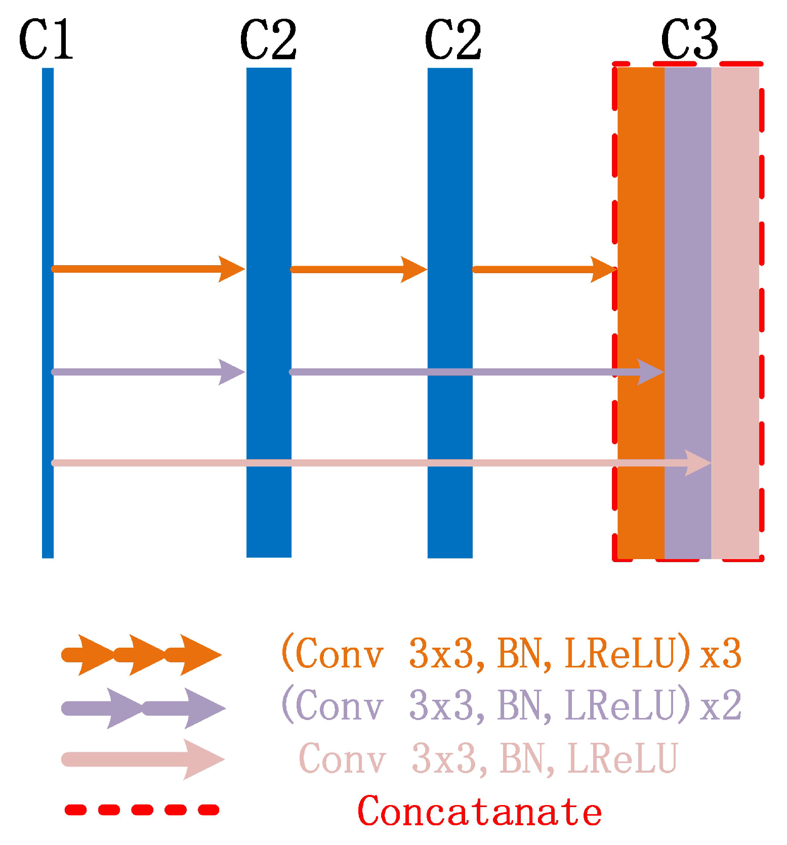
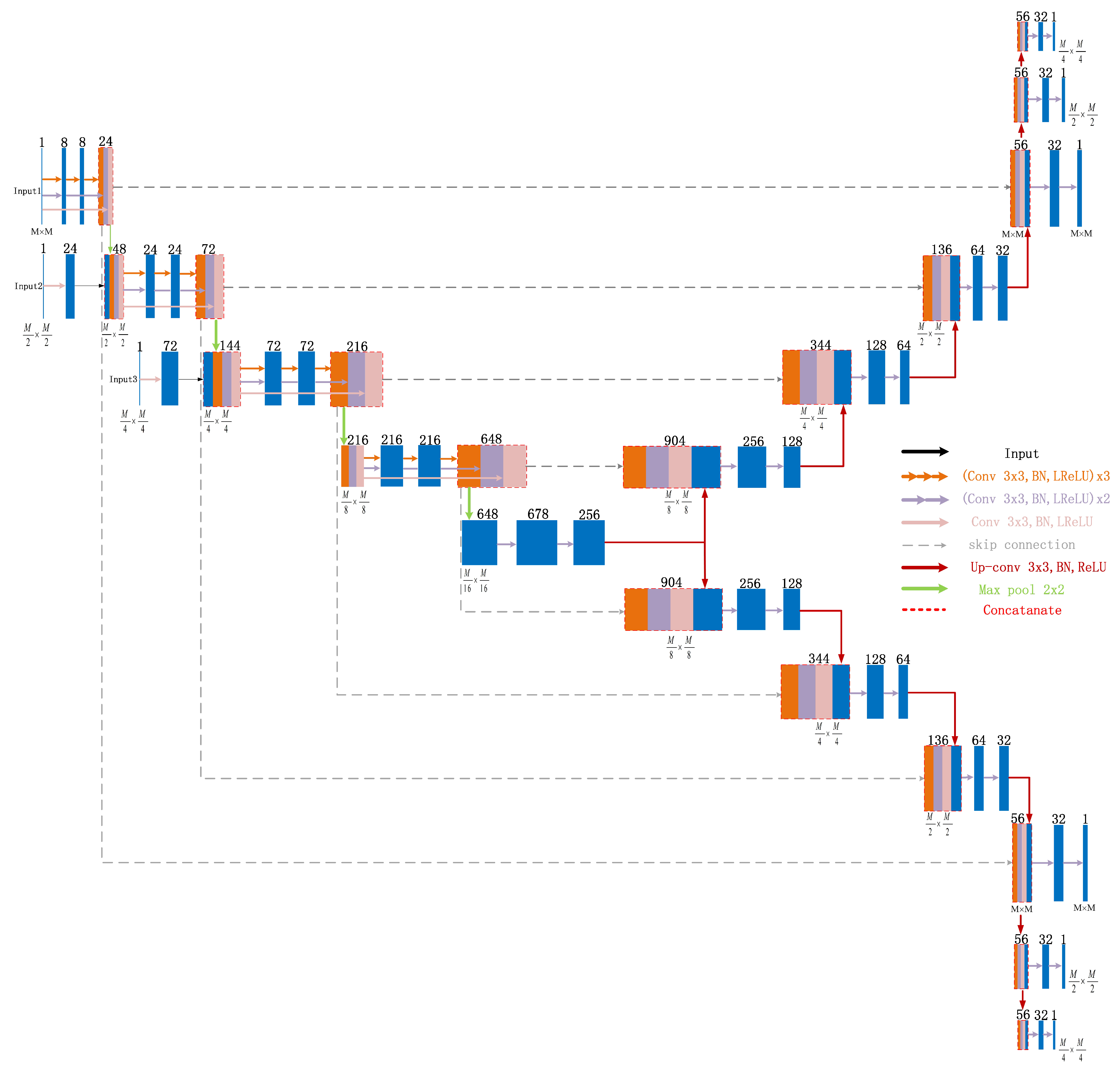
2.3. Mimo-Net Network Structure

Deep-learning-based hologram reconstruction methods have received widespread attention [27,28,29], among which the Y-Net is a particularly significant class [30]. The Mimo-Net proposed in this paper consists of the Y-Net, a multiscale feature-extraction module, and multiscale reconstruction fusion. The network structure is symmetric and can satisfy different requirements. As shown in Figure 2, the Mimo-Net consists of one down-sampling path, two up-sampling paths (one for intensity and one for phase), and skip links.

(1) The down-sampling path consists of a multiscale feature-extraction module and a max-pooling layer, which can gradually reduce the size of the feature maps while increasing the level of feature abstraction.

(2) Multiscale feature-extraction module. As shown in Figure 3, it consists of three parallel convolutional layers and cascades of small convolutional kernels for feature extraction. Three feature maps are extracted using single 3 × 3 convolution, double 3 × 3 convolutions, and triple 3 × 3 convolutions. Batch normalization (BN) [31] and activation function [32] are applied to reduce internal covariate shift and speed up network training. Choosing Leaky Rectified Linear Unit (LReLU) as the activation function can reduce the oscillation and better fit the model. Finally, the feature maps from the three branches are concatenated. In the convolution layer, the series of two 3 × 3 convolution layers is equivalent to one 5 × 5 convolution layer, the series of three 3 × 3 convolution layers is equivalent to one 7 × 7 convolution layer, and the receptive field size of three 3 × 3 convolution layers is equivalent to one 7 × 7 convolution layer. However, the number of parameters of three 3 × 3 convolution layers is only about half that of 7 × 7, and the former can have three nonlinear operations, while the latter has only one nonlinear operation, which makes the former have stronger feature learning ability [33]. The multiscale feature-extraction module deepens the model with increased non-linearity and improved learning capacity. This results in a more extensive representation space and more vital feature-extraction capability, efficiently extracting features of different sizes in holograms.

(3) Multiscale reconstruction. In the leading hologram feature-extraction network, three input branches are sequentially constructed to extract multiscale features and perform feature fusion, as shown in Figure 3. In this network, holograms of three different scales are selected: 256 × 256, 128 × 128, and 64 × 64. The 256 × 256 scale hologram is used as the input for multiscale feature extraction in the leading network. After the maximum pooling layer with a kernel size of 2 × 2, the scale is reduced by half. Another branch is added, with the same input channels, where the 128 × 128 hologram is merged with the down-sampled image for further multiscale feature extraction and max-pooling. Another branch is added, with the same input channels, where the 64 × 64 hologram is merged with the down-sampled image for further down-sampling learning. Each down-sampling and corresponding up-sampling performs feature fusion. The up-sampling output undergoes multiple max-pooling and convolution operations, resulting in three outputs that simultaneously produce intensity and phase information at 256 × 256, 128 × 128, and 64 × 64 scales. Max-pooling is used to preserve edge detail, multiscale input is used to increase the receptive field of the model, and feature fusion is used to incorporate complementary information. Throughout the process, large-scale and small-scale feature extraction reinforce each other to achieve multiscale feature learning and quickly obtain global features while extracting detailed features.

(4) Up-sampling path. The Mimo-Net network in this paper has two symmetric up-sampling paths, which extract intensity and phase information, respectively, to restore resolution and achieve dual-channel output. Deconvolution is used to restore the image to its original size after four rounds of up-sampling. This process uses a cascaded 3 × 3 convolution, reducing the number of channels by half. It uses the concatenation of feature maps with the exact dimensions to improve resolution.

(5) Skip connections. The down-sampled feature maps are connected to the corresponding up-sampled paths via skip connections. In the Mimo-Net network proposed in this paper, skip connections are applied after the fusion of multiple input features, enabling information exchange between different inputs and integrating multiscale information. This effectively solves performance degradation problems in deep networks and ensures stable network training.

3. Experiment and Result Analysis

Three sets of experiments were carried out. Under the same conditions, the Y-Net model was used for three reconstructions with scales of 256 × 256, 128 × 128, and 64 × 64, while the Mimo-Net model was used for a single reconstruction with scales of 256 × 256, 128 × 128, and 64 × 64. The results of the two models were then compared.

3.1. Experiment Setup and Dataset Generation

The experimental platform is based on the Windows 10 operating system. The experimental configuration is shown in

Table 1. Experimental environment.

Hardware Configuration	Parameter
CPU	i5 9400F
RAM	32G
GPU	RTX3060
GPU Memory	12G
Framework	TensorFlow2.0

. The programming software used is Python 3.9. During the experimental training process, the epoch is set to 100, the batch size is set to 10, and the Adam optimizer [34] and RMSE loss function are selected for the experiment.

Digital holograms are created through the interference of objects and reference light. Digital hologram datasets are generated through computer algorithms that simulate holographic diffraction and interference. We have selected from a dataset of handwritten images such that 12,000 images are evenly divided into two folders. The images in the first folder are then enlarged to the corresponding scale, and normalized to obtain their intensity information. The images in the second folder are magnified to match the intensity scale and then normalized [35] for phase processing. To obtain the distribution of object amplitudes, the object undergoes phase modulation. Interfering with the reference light wave with the object plane diffraction field results in 6000 digital holograms with a scale of 256 × 256. Performing subsequent local feature extractions retains the important information from the center of each hologram, with scales of 128 × 128 and 64 × 64, respectively. Figure 4 displays the procedure used for local feature extraction. In total, 6000 digital holograms of 256 × 256, 128 × 128, and 64 × 64 scale were obtained. From each scale, 4800 holograms were chosen for the training set and 1200 for the test set.

3.2. Evaluation Index

The root mean square error (RMSE) is a frequently applied loss function in deep learning. In a dataset, it is the square root of the mean of the squared differences between the actual and predicted values. It offers an intuitive way to gauge the difference between the actual data and real values. The formula for RMSE is Equation (7):

$$\begin{array}{c}RMSE=\sqrt{\frac{1}{N}{\displaystyle \sum _{i=1}^N}{(\stackrel{\wedge }{y_i}-y_i)}^2}\hfill \end{array},$$

(7)

When training neural networks with multi-task learning and multi-objective optimization, it is necessary to balance multiple loss functions [36]. The loss functions for the intensity and phase images are:

$$\begin{array}{c}{L}_I=\sqrt{\frac{1}{N}{\displaystyle \sum _i^N}{∥\stackrel{\wedge }{I_i}-I_i∥}^2}\hfill \end{array},$$

(8)

$$\begin{array}{c}{L}_P=\sqrt{\frac{1}{N}{\displaystyle \sum _i^N}{∥\stackrel{\wedge }{P_i}-P_i∥}^2}\hfill \end{array},$$

(9)

The equation uses $\stackrel{\wedge }{I_i}$ and $I_i$ to represent the real intensity image and reconstructed intensity image, respectively, additionally $\stackrel{\wedge }{P_i}$ and $P_i$ represent the real phase image and reconstructed phase image, respectively. The symbol i denotes the number of training data samples, and N represents the size of the sampling. To balance multi-task optimization and strengthen the relationship between the intensity and phase images, the loss function computes a weighted sum to allow backpropagation through the neural network.

If the Y-Net network model is optimized for two tasks, the loss function is as follows:

$$\begin{array}{c}{L}_{IP}={\lambda }_1{L}_I+{\lambda }_2{L}_P\hfill \end{array},$$

(10)

Reference [20] states that for Y-Net, the loss function weight values are ${\lambda }_1$ = 0.01 and ${\lambda }_2$ = 1. When optimizing the Mimo-Net network model for the six tasks, the loss function can be expressed as Equations (11):

$$\begin{array}{c}{L}_{IP}={\lambda }_1{L}_{I1}+{\lambda }_1{L}_{I2}+{\lambda }_1{L}_{I13}+{\lambda }_2{L}_{P1}+{\lambda }_2{L}_{P2}+{\lambda }_2{L}_{P3}\hfill \end{array},$$

(11)

Here, $L_{I1}$, $L_{I2}$ and $L_{I3}$ represent the mean squared errors of intensity images with scales of 256 × 256, 128 × 128, and 64 × 64, respectively, $L_{P1}$, $L_{P2}$ and $L_{P3}$ represent the mean squared errors of phase images with scales of 256 × 256, 128 × 128, and 64 × 64, respectively. The weight of the intensity loss function is denoted as ${\lambda }_1$, and the weight of the phase loss function is denoted as ${\lambda }_2$. During training, it is necessary to minimize the comprehensive loss of all tasks by assigning different weights to each task. This helps to achieve the minimum total loss function $L_{IP}$.

A set of optimal weights is chosen as ${\lambda }_1=0.0005$, ${\lambda }_2=0.01$ after continuous testing and training.

3.3. Experimental Results and Analysis

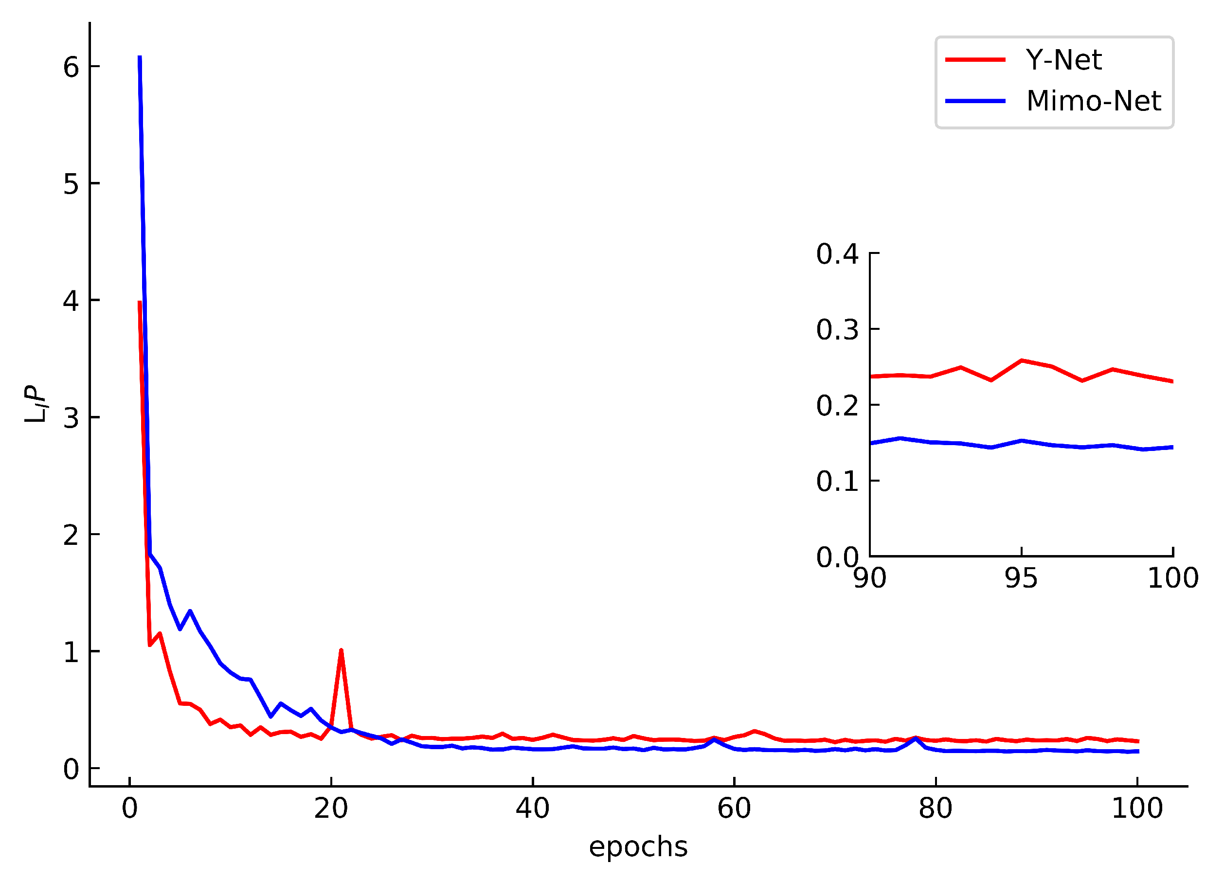
3.3.1. Comparison of Mimo-Net and Y-Net Training Results

Under the same software and hardware environment and dataset conditions, using 256 × 256, 128 × 128, and 64 × 64 scale datasets to train the Mimo-Net network model, the Mimo-Net test set loss is obtained. Y-Net network models were trained on datasets of 256 × 256, 128 × 128, and 64 × 64 scales, respectively, and the average test set losses of the three models were calculated. The comparative curve of test set losses for both network models is shown in Figure 5, where the y-axis represents the $L_{IP}$ and the x-axis represents the epochs, ranging from 0 to 100. When the models reached an epoch value of 20, the Mimo-Net network showed a relatively stable trend, while the Y-Net network still showed more significant fluctuations. On the right side of the figure, with epoch values ranging from 90 to 100, the loss values of both networks are amplified for comparison. The Mimo-Net network has better overall convergence, accuracy, and stability, indicating successful training. The final loss value for Mimo-Net tends to be closer to 0.15, while for Y-Net it tends to be closer to 0.23. The Mimo-Net network shows an improvement in accuracy of 34.78%.

Record training time for Y-Net and Mimo-Net. Y-Net requires three training rounds to reconstruct intensity and phase information at three different scales. Mimo-Net, on the other hand, only needs to be trained once to reconstruct intensity and phase information simultaneously at scales of 256 × 256, 128 × 128, and 64 × 64. The recorded times are shown in

Table 2. Y-Net and Mimo-Net reconstruct the training time of intensity and phase information at three scales.

Net	Scales	Times/s	Total Times/s
	256 × 256	1687
Y-Net	128 × 128	582	2713
	64 × 64	444
Mimo-Net	256 × 256, 128 × 128, 64 × 64	1008	1008

.

Table 2 shows that training Y-Net to reconstruct intensity and phase information at three different scales took 2713 s, while Mimo-Net reconstruction took 1008 s. Therefore, the reconstruction time of the Mimo-Net network was reduced by 62%, leading to an improvement in reconstruction efficiency.

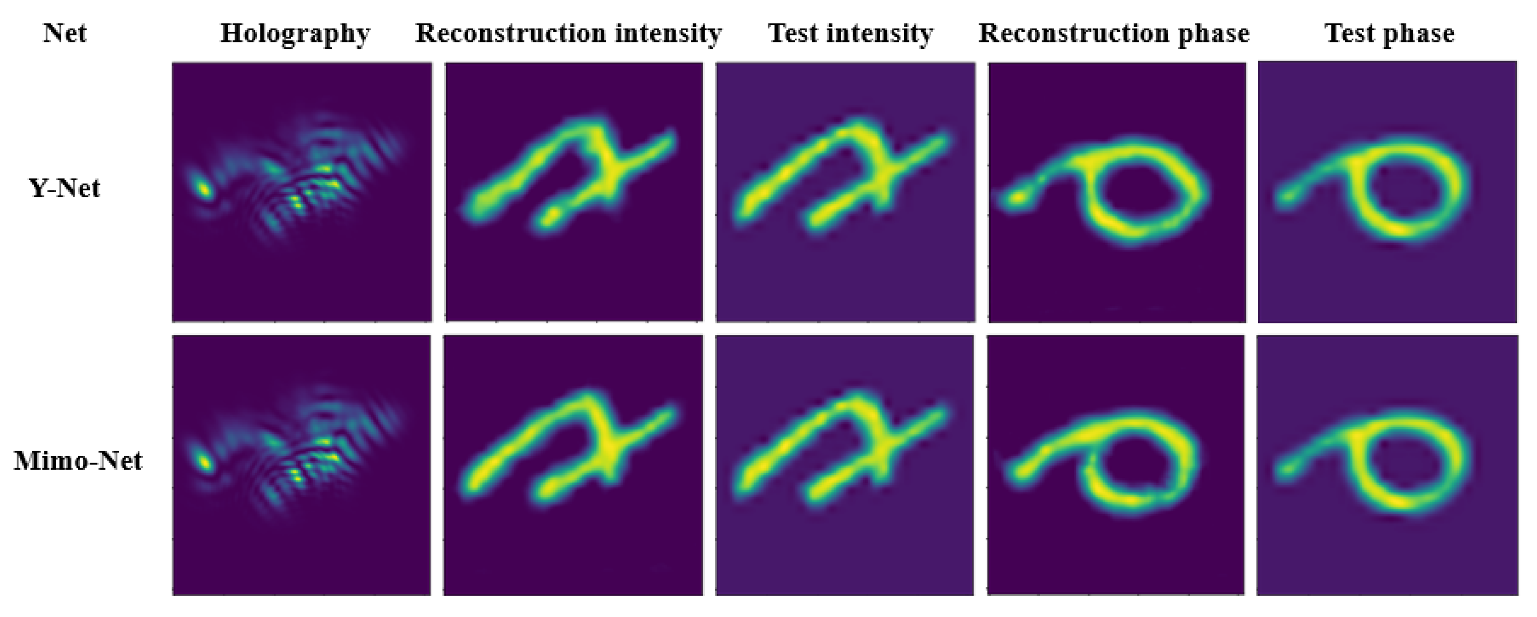
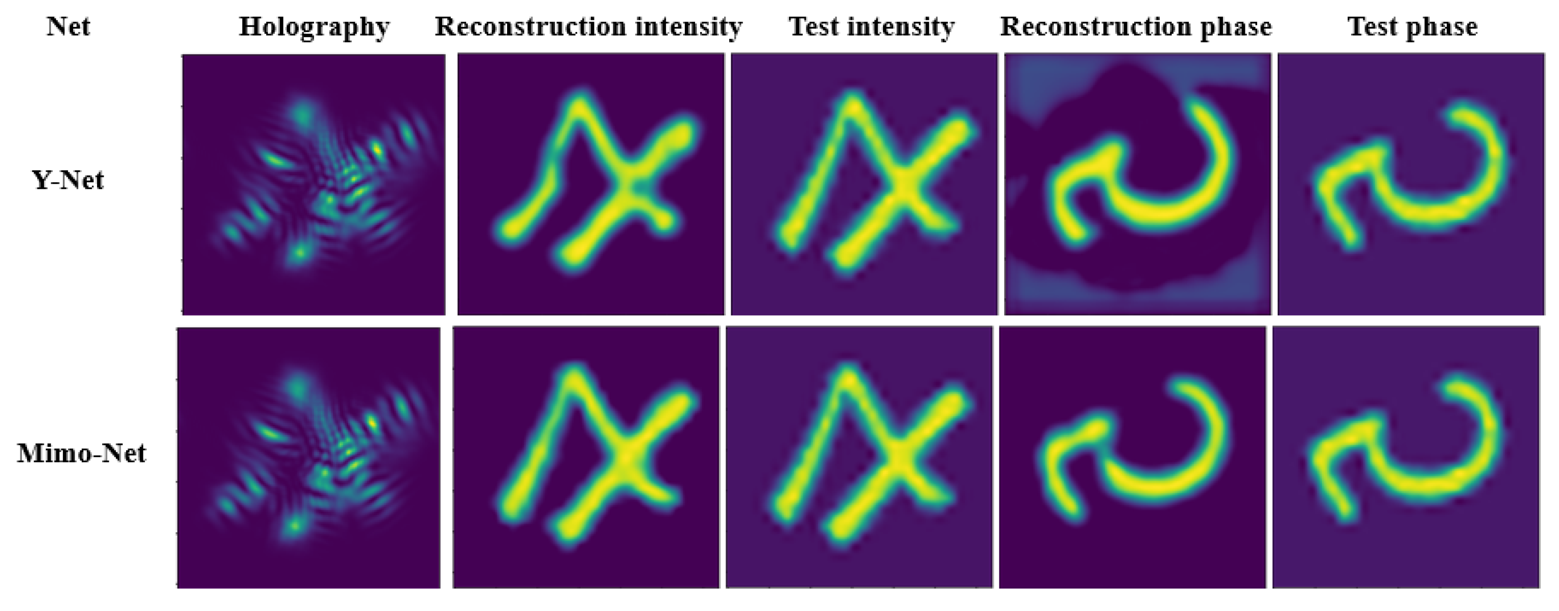
3.3.2. Comparison of Mimo-Net and Y-Net at 256 × 256 Scale

The reconstructed results of the Mimo-Net and Y-Net models were compared using images at 256 × 256-scale, the enlarged comparison figures are shown in Figure 6.

Figure 6 shows that the intensity and phase images reconstructed by the proposed Mimo-Net network have better results than the reconstructed images from the Y-Net network.

Table 3. 256 × 256 scale PSNR and SSIM.

Parameter	Intensity of Y-Net	Intensity of Mimo-Net	Phase of Y-Net	Phase of Mimo-Net
PSNR/dB	31.5431	33.9632	31.0891	31.3922
SSIM	0.9251	0.9463	0.9208	0.9252

shows the peak signal-to-noise ratio (PSNR) and structural similarity (SSIM) between the reconstructed images from the Mimo-Net and Y-Net networks and the original images.

Table 3 shows that the Mimo-Net network model has improved the PSNR of the reconstructed intensity and phase images by 2.4201 dB and 0.3031 dB, respectively, compared to the Y-Net network. The SSIM values have also increased by 0.0212 and 0.0044, respectively. Therefore, the Mimo-Net network exhibits better reconstruction performance.

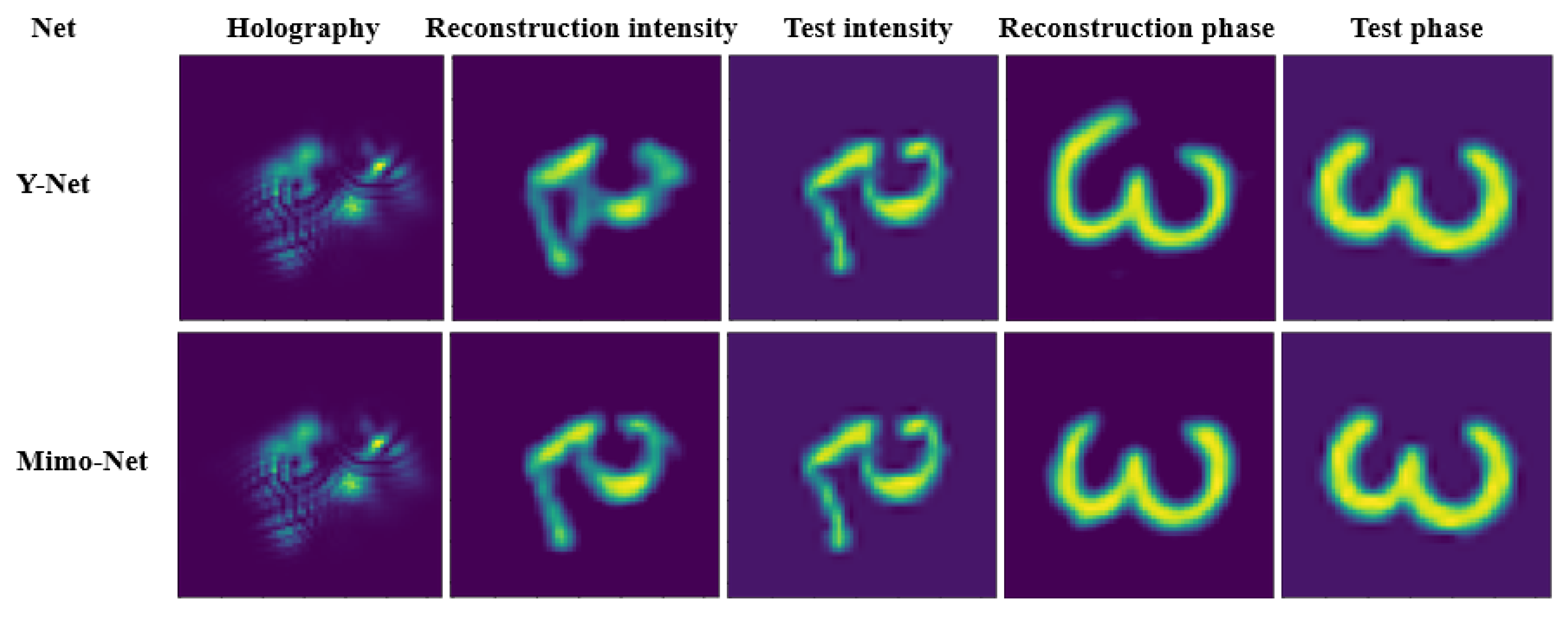
3.3.3. Comparison of Mimo-Net and Y-Net at 128 × 128 Scale

The reconstructed results of the Mimo-Net and Y-Net models were compared using images at 128 × 128 scale, the enlarged comparison figures are shown in Figure 7.

Figure 7 shows that the intensity image reconstructed by the proposed Mimo-Net network is better improved than that reconstructed by the Y-Net network, and the phase image is also improved

Table 4. 128 × 128 scale PSNR and SSIM.

Parameter	Intensity of Y-Net	Intensity of Mimo-Net	Phase of Y-Net	Phase of Mimo-Net
PSNR/dB	29.7061	32.4975	31.3524	31.5966
SSIM	0.9499	0.9676	0.9239	0.9403

shows the PSNR and SSIM values of the images reconstructed by the Mimo-Net network and the Y-Net network compared to the original images.

Table 4 shows that the strength and phase images reconstructed by the Mimo-Net network model have improved PSNR values by 2.7914 dB and 0.0177 dB, respectively, compared to the Y-Net network. The SSIM values have also increased by 0.2442 and 0.0164, respectively. Therefore, the Mimo-Net network exhibits better reconstruction performance.

3.3.4. Comparison of Mimo-Net and Y-Net at 64 × 64 Scale

The reconstructed results of the Mimo-Net and Y-Net models were compared using images at 64 × 64-scale, the enlarged comparison figures are shown in Figure 8.

Figure 8 shows that the intensity image of Y-Net network reconstruction is incomplete, with burrs and protrusions at the edge of the phase image, while the intensity and phase images of Mimo-Net network reconstruction are relatively complete, and the reconstruction effect is also improved.

Table 5. 64 × 64 scale PSNR and SSIM.

Parameter	Intensity of Y-Net	Intensity of Mimo-Net	Phase of Y-Net	Phase of Mimo-Net
PSNR/dB	29.5614	31.9453	28.4567	29.5390
SSIM	0.8794	0.9249	0.8943	0.9320

presents the PSNR and SSIM values of the images reconstructed by the Mimo-Net network and the Y-Net network compared to the original images.

Table 5 shows that the strength and phase images reconstructed by the Mimo-Net network model have improved PSNR values by 2.3839 dB and 1.0823 dB, respectively, compared to the Y-Net network. The SSIM values have also increased by 0.0455 and 0.0377, respectively. Therefore, the Mimo-Net network exhibits better reconstruction performance.

4. Summary and Analysis

This paper proposes an improved deep-learning model called Mimo-Net, which achieves the reconstruction of both intensity and phase information of three-scale digital holograms using a single network architecture. For digital holograms with concentrated useful information, feature extraction can be performed from global to local scales to reconstruct three-scale digital holograms, capturing feature information from different receptive fields and better integrating features of different scales. Compared to the Y-Net model, the Mimo-Net model only needs to be trained once to reconstruct the intensity and phase of three different-scale digital holograms. Through comparative experiments, the Mimo-Net network demonstrates higher accuracy in the reconstruction process compared to the Y-Net network, indicating the effectiveness of the proposed network model. However, the structural similarity and peak signal-to-noise ratio of the reconstructed phase information are not satisfactory compared to the reconstructed intensity information. Further improvements are needed in the network structure and parameters to enhance the accuracy of the reconstructed phase information while ensuring high precision and reducing hardware requirements for the network.

References

1. Sheridan, J.T.; Kostuk, R.K.; Gil, A.F.; Wang, Y.; Lu, W.; Zhong, H.; Tomita, Y.; Neipp, C.; Francés, J.; Gallego, S.; et al. Roadmap on holography. J. Opt. 2020, 22, 123002. [Google Scholar] [CrossRef]
2. Chernykh, A.V.; Ezerskii, A.S.; Georgieva, A.O.; Petrov, N.V. Study on object wavefront sensing in parallel phase-shifting camera with geometric phase lens. In Proceedings of the SPIE, San Diego, CA, USA, 1–5 August 2021; Volume 11898, p. 118980X. [Google Scholar]
3. Kim, M.K. Principles and techniques of digital holographic microscopy. SPIE Rev. 2010, 1, 018005. [Google Scholar] [CrossRef]
4. Rabosh, E.V.; Balbekin, N.S.; Timoshenkova, A.M.; Shlykova, T.V.; Petrov, N.V. Analog-to-digital conversion of information archived in display holograms: II. photogrammetric digitization. JOSA A 2023, 40, B57–B64. [Google Scholar] [CrossRef]
5. Marquet, P.; Rappaz, B.; Magistretti, P.J.; Cuche, E.; Emery, Y.; Colomb, T.; Depeursinge, C. Digital holographic microscopy: A noninvasive contrast imaging technique allowing quantitative visualization of living cells with subwavelength axial accuracy. Opt. Lett. 2005, 30, 468–470. [Google Scholar] [CrossRef]
6. Stepanishen, P.R.; Benjamin, K.C. Forward and backward projection of acoustic fields using FFT methods. J. Acoust. Soc. Am. 1982, 71, 803–812. [Google Scholar] [CrossRef]
7. Dyomin, V.; Davydova, A.; Kirillov, N.; Polovtsev, I. Features of the Application of Coherent Noise Suppression Methods in the Digital Holography of Particles. Appl. Sci. 2023, 13, 8685. [Google Scholar] [CrossRef]
8. LeCun, Y.; Bengio, Y.; Hinton, G. Deep learning. Nature 2015, 521, 436–444. [Google Scholar] [CrossRef] [PubMed]
9. Zhao, F.; Zhu, L.; Fang, C.; Yu, T.; Zhu, D.; Fei, P. Deep-learning super-resolution light-sheet add-on microscopy (Deep-SLAM) for easy isotropic volumetric imaging of large biological specimens. Biomed. Opt. Express 2020, 11, 7273–7285. [Google Scholar] [CrossRef] [PubMed]
10. Bochkovskiy, A.; Wang, C.Y.; Liao, H.Y.M. Yolov4: Optimal speed and accuracy of object detection. arXiv 2020, arXiv:2004.10934. [Google Scholar]
11. Huang, Y.; Lu, Z.; Shao, Z.; Ran, M.; Zhou, J.; Fang, L.; Zhang, Y. Simultaneous denoising and super-resolution of optical coherence tomography images based on generative adversarial network. Opt. Express 2019, 27, 12289–12307. [Google Scholar] [CrossRef] [PubMed]
12. Svistunov, A.S.; Rymov, D.A.; Starikov, R.S.; Cheremkhin, P.A. HoloForkNet: Digital Hologram Reconstruction via Multibranch Neural Network. Appl. Sci. 2023, 13, 6125. [Google Scholar] [CrossRef]
13. Zhang, G.; Guan, T.; Shen, Z.; Wang, X.; Hu, T.; Wang, D.; He, Y.; Xie, N. Fast phase retrieval in off-axis digital holographic microscopy through deep learning. Opt. Express 2018, 26, 19388–19405. [Google Scholar] [CrossRef]
14. Ren, Z.; Xu, Z.; Lam, E.Y. End-to-end deep learning framework for digital holographic reconstruction. Adv. Photonics 2019, 1, 016004. [Google Scholar] [CrossRef]
15. Xiao, W.; Wang, Q.; Pan, F.; Cao, R.; Wu, X.; Sun, L. Adaptive frequency filtering based on convolutional neural networks in off-axis digital holographic microscopy. Biomed. Opt. Express 2019, 10, 1613–1626. [Google Scholar] [CrossRef]
16. Barbastathis, G.; Ozcan, A.; Situ, G. On the use of deep learning for computational imaging. Optica 2019, 6, 921–943. [Google Scholar] [CrossRef]
17. Sinha, A.; Lee, J.; Li, S.; Barbastathis, G. Lensless computational imaging through deep learning. Optica 2017, 4, 1117–1125. [Google Scholar] [CrossRef]
18. Rivenson, Y.; Zhang, Y.; Günaydın, H.; Teng, D.; Ozcan, A. Phase recovery and holographic image reconstruction using deep learning in neural networks. Light. Sci. Appl. 2018, 7, 17141. [Google Scholar] [CrossRef]
19. Wang, H.; Lyu, M.; Situ, G. eHoloNet: A learning-based end-to-end approach for in-line digital holographic reconstruction. Opt. Express 2018, 26, 22603–22614. [Google Scholar] [CrossRef]
20. Wang, K.; Dou, J.; Kemao, Q.; Di, J.; Zhao, J. Y-Net: A one-to-two deep learning framework for digital holographic reconstruction. Opt. Lett. 2019, 44, 4765–4768. [Google Scholar] [CrossRef]
21. Picart, P.; Li, J.C. Digital Holography; John Wiley & Sons: Hoboken, NJ, USA, 2013. [Google Scholar]
22. Benton, S.A.; Bove, V.M., Jr. Holographic Imaging; John Wiley & Sons: Hoboken, NJ, USA, 2008. [Google Scholar]
23. Schnars, U.; Jüptner, W. Direct recording of holograms by a CCD target and numerical reconstruction. Appl. Opt. 1994, 33, 179–181. [Google Scholar] [CrossRef]
24. Kreis, T.M.; Adams, M.; Jüptner, W.P. Methods of digital holography: A comparison. In Proceedings of the Optical Inspection and Micromeasurements II, SPIE, Munich, Germany, 16–19 June 1997; Volume 3098, pp. 224–233. [Google Scholar]
25. Grilli, S.; Ferraro, P.; De Nicola, S.; Finizio, A.; Pierattini, G.; Meucci, R. Whole optical wavefields reconstruction by digital holography. Opt. Express 2001, 9, 294–302. [Google Scholar] [CrossRef] [PubMed]
26. Georgieva, A.; Ezerskii, A.; Chernykh, A.; Petrov, N. Numerical displacement of target wavefront formation plane with DMD-based modulation and geometric phase holographic registration system. Atmos. Ocean. Opt. 2022, 35, 258–265. [Google Scholar] [CrossRef]
27. Zeng, T.; Zhu, Y.; Lam, E.Y. Deep learning for digital holography: A review. Opt. Express 2021, 29, 40572–40593. [Google Scholar] [CrossRef] [PubMed]
28. Rivenson, Y.; Wu, Y.; Ozcan, A. Deep learning in holography and coherent imaging. Light. Sci. Appl. 2019, 8, 85. [Google Scholar] [CrossRef] [PubMed]
29. Park, S.; Kim, Y.; Moon, I. Automated phase unwrapping in digital holography with deep learning. Biomed. Opt. Express 2021, 12, 7064–7081. [Google Scholar] [CrossRef]
30. Vithin, A.V.S.; Vishnoi, A.; Gannavarpu, R. Phase derivative estimation in digital holographic interferometry using a deep learning approach. Appl. Opt. 2022, 61, 3061–3069. [Google Scholar] [CrossRef]
31. Ioffe, S.; Szegedy, C. Batch normalization: Accelerating deep network training by reducing internal covariate shift. In Proceedings of the International Conference on Machine Learning, PMLR, Lille, France, 6–11 July 2015; pp. 448–456. [Google Scholar]
32. Hara, K.; Saito, D.; Shouno, H. Analysis of function of rectified linear unit used in deep learning. In Proceedings of the 2015 International Joint Conference on Neural Networks (IJCNN), Killarney, Ireland, 12–17 July 2015; pp. 1–8. [Google Scholar]
33. Wang, L.; Li, Y.; Wang, S. DeepDeblur: Fast one-step blurry face images restoration. arXiv 2017, arXiv:1711.09515. [Google Scholar]
34. Kingma, D.P.; Ba, J. Adam: A method for stochastic optimization. arXiv 2014, arXiv:1412.6980. [Google Scholar]
35. Morgan, H.; Druckmüller, M. Multi-scale Gaussian normalization for solar image processing. Sol. Phys. 2014, 289, 2945–2955. [Google Scholar] [CrossRef]
36. Chen, C.; Lee, B.; Li, N.N.; Chae, M.; Wang, D.; Wang, Q.H.; Lee, B. Multi-depth hologram generation using stochastic gradient descent algorithm with complex loss function. Opt. Express 2021, 29, 15089–15103. [Google Scholar] [CrossRef]
Figure 1. Digital hologram system model.
Applsci 13 09806 g001
Figure 2. Mimo-Net architecture. There are three inputs on the left and six outputs (intensity and phase) on the right. The pink arrow represents the 3 × 3 convolution, the purple arrow represents the double 3 × 3 convolution, and the pink arrow represents the triple 3 × 3 convolution. Each block has the number of channels and the size of the feature map.
Applsci 13 09806 g002
Figure 3. Multi-feature-extraction module. C1, C2, and C3 indicate the number of channels, which represents the quantity of different learned features. Parallel convolution followed by concatenation.
Applsci 13 09806 g003
Figure 4. Local feature-extraction process. From 256 × 256 scales to 128 × 128 scales to 64 × 64 scales.
Applsci 13 09806 g004
Figure 5. Comparison image of test set loss values between Y-Net and Mimo-Net networks.
Applsci 13 09806 g005
Figure 6. Comparison of Mimo-Net and Y-Net network reconstruction results at 256 × 256 scale.
Applsci 13 09806 g006
Figure 7. Comparison of Mimo-Net and Y-Net network reconstruction results at 128 × 128 scale.
Applsci 13 09806 g007
Figure 8. Comparison of Mimo-Net and Y-Net network reconstruction results at 64 × 64 scale.
Applsci 13 09806 g008