Electric Load Forecasting Based on Deep Ensemble Learning

Abstract

Short-to-medium-term electric load forecasting is crucial for grid planning, transformation, and load scheduling for power supply departments. Various complex and ever-changing factors such as weather, seasons, regional economic structures, and enterprise production cycles exert uncontrollable effects on the electric grid load. While the causal convolutional neural network can significantly enhance long-term sequence prediction, it may suffer from problems such as vanishing gradients and overfitting due to extended time series. To address this issue, this paper introduces a new power load data anomaly detection method, which leverages a convolutional neural network (CNN) to extract temporal and spatial information from the load data. The features extracted are then processed using a bidirectional long short-term memory network (BiLSTM) to capture the temporal dependencies in the data more adeptly. An enhanced random forest (RF) classifier is employed for anomaly detection in electric load data. Furthermore, the paper proposes a new model framework for electricity load forecasting that combines a dilated causal convolutional neural network with ensemble learning. This combination addresses issues such as vanishing gradients encountered in causal convolutional neural networks with long time series. Extreme gradient boosting (XGBoost), category boosting (CATBoost), and light gradient boosting machine (LightGBM) models act as the base learners for ensemble modeling to comprehend deep cross-features, and the prediction results generated by ensemble learning serve as a new feature set for secondary ensemble modeling. The dilated convolutional neural network broadens the receptive field of the convolutional kernel. All acquired feature values are concatenated and input into the dilated causal convolutional neural network for training, achieving short-to-medium-term electric load forecasting. Experimental results indicate that compared to existing models, its root mean squared error (RMSE) and mean squared error (MSE) in short-term and mid-term electricity load forecasting are reduced by 4.96% and 12.31%, respectively, underscoring the efficacy of the proposed framework.

1. Introduction

Power system load forecasting, which encompasses power demand and active power predictions, involves predicting future system loads based on historical data, weather conditions, and the implications of current policies and regulations [1]. Electricity load forecasting is essential in power planning, transmission, and distribution within the grid sector. Short-term forecasts (less than two weeks) form the foundation for unit start-ups and shutdowns and scheduling and operational plans within the grid. Medium-term forecasts (spanning several months) can guide rational grid operation and maintenance decisions, ensuring consistent electricity supply for businesses and everyday life; these forecasts also offer a valuable foundation for grid operation and scheduling decisions across different industries. Long-term forecasts (looking years ahead) provide data vital for decision making concerning the grid system’s renewal and transformation, aiming to enhance societal benefits. By predicting the electrical load for businesses, large industries, specialized industries, and general industries, one can understand the operational status of each sector, which in turn aids in the resumption and subsequent growth of enterprises.

Forecasting and analyzing the power output of regional power systems allows for accurate electricity supply [2]. By systematically analyzing electricity consumption forecast data, power supply companies can plan and allocate future electric energy more effectively, enhancing the precision and efficiency of their planning. This approach helps avoid issues like blind, transitional, or insufficient power planning. Moreover, electricity consumption can also serve as an indicator of local economic development. By utilizing electricity forecasting, government departments can obtain valuable insights into economic growth, which can subsequently inform and support the formulation of government economic policies.

Complex factors, such as volatile climate conditions, can introduce uncontrollable effects on power load forecasting, rendering traditional models’ predictions uncertain. As power systems evolve, their structural levels become more diverse, necessitating further research into the challenges of power load forecasting.

1.1. Related Works

Power load forecasting can be categorized into traditional and intelligent methods. Traditional methods typically encompass the elasticity coefficient, consumption unit, catalog, and load density methods [3]. While these methods are not sufficiently accurate for prediction, some power companies still employ them due to practical considerations. Techniques such as regression analysis and time series analysis are also used for daily forecasting. Further details are provided below.

1.1.1. Traditional Forecasting Methods

Regression analysis involves the establishment of a regression equation to predict the future trend of the dependent variable based on the analysis of both dependent and independent variables. This model is straightforward to construct and offers quick predictions. For instance, in 2021, Gong et al. [4] introduced a kernel function to the lasso linear regression method, applying it to nonlinear problems to address the regression analysis of non-time series data. Its accuracy improved compared to standard lasso regression, yielding enhanced results. Wang et al. [5], in their research, introduced a hybrid support vector regression approach. They investigated the coupling and inter-dependency between the model parameters. Moreover, they optimized the hyper-parameters and altered the model’s configuration using nested strategies and state-transformation algorithms. This method was successfully applied to predict medium- and long-term electric loads in a real industry in China. The essence of the regression method is to analyze vast amounts of actual data to understand the relationship between these factors and the electric load. The goal is to use this relationship to predict the future trajectory of the electric load. These influencing factors are straightforward to analyze and understand, and the prediction accuracy is commendably high. However, these influencing factors can change due to environmental shifts, policy alterations, and other uncertainties. These elements introduce a high degree of randomness. If anomalous data are used as the foundation for prediction, they can adversely affect the accuracy of future power load forecasts.

The time series method is an illustrative approach based on historical electricity data. The amount of data required for this method allows for electricity forecasting without the need for an enormous scale. For example, In 2021, Chodakowska. E. et al. [6] investigated the impact of noise on the inadequate identification of autoregressive integrated moving average (ARIMA) model factors and proposed a series of solutions. They experimented with actual power load samples derived from Poland, evaluating the robustness of ARIMA models to noise in predicting the time series of electric loads. Additionally, they determined the limiting noise level for predictive capability. Time series are ordered sequences of data points over time, and they predict future changes based on past electricity loads. One advantage of this model is its simplicity in understanding and execution. However, if forecasting relies solely on changes in electricity loads, achieving accurate predictions becomes challenging. This is mainly because electricity loads exhibit randomness and seasonality, making the forecast less than ideal.

1.1.2. Intelligent Forecasting Methods

Intelligent forecasting models encompass machine learning and its subfield, deep learning. Machine learning is a field of artificial intelligence, with its central idea being to allow computers to learn patterns and regularities from data, enabling tasks such as prediction, classification, and clustering. Through machine learning, computers can automatically uncover valuable information from vast amounts of data, thereby assisting in decision making, enhancing efficiency, and solving complex problems. Deep learning is a subset of machine learning and represents a significant branch. This contemporary technique builds upon traditional neural networks, offering enhanced classification and prediction accuracy. Intelligent methods are widely acknowledged in academia and industry [7] and have applications in the electrical fields. For example, Ke et al. [8] established a prediction model based on the genetic algorithm-backpropagation (GA-BP) neural network. They formed a continuous linear time series for training by incorporating a sliding window and other techniques. This approach mitigated the overfitting problem often seen with more traditional methods and demonstrated that the proposed framework achieved higher forecasting accuracy than conventional methods. Xia et al. [9] designed a short-term load forecasting method for power systems based on gradient boosting trees. This method preprocesses data by quantifying short-term load-influencing factors using fuzzy probabilities, applies difference decomposition to handle short-term load data, and establishes a robust regression gradient boosting tree in the direction of the negative gradient of the loss function to obtain the load forecasting results. Tasarruf et al. [10] proposed a hybrid approach utilizing both the Prophet and long short-term memory (LSTM) models. Initially, the Prophet model forecasts the raw load data by leveraging both linear and nonlinear data. However, some nonlinear data remain, which are then trained using the LSTM. Ultimately, the predictive outputs from both the Prophet and LSTM are trained through a backpropagation neural network (BPNN) to further enhance the prediction accuracy. Wu et al. [11] proposed an attention-based convolutional neural network (CNN) model that combines both LSTM and bidirectional long short-term memory (BiLSTM). By utilizing CNN and the attention mechanism, we extract key factors influencing the load. Subsequently, the LSTM and BiLSTM are employed to forecast future electricity load data. Aguilar Madrid et al. [12] proposed a set of machine learning (ML) models to enhance the accuracy of electric load forecasting, including multiple linear regression (MLR), k-nearest neighbor regressor (KNN), epsilon support vector regression (SVR), the random forest regressor (RF), and the extreme gradient boosting regressor (XGB). Experiments show that the model constructed using XGB outperforms those built with other algorithms. Lin et al. [13] employed an attention-based LSTM network model for electric load forecasting. Firstly, they constructed a feature-based attention encoder to compute the correlation between input features at each time step and the electric load. Secondly, they developed a time-based attention decoder to delve into temporal dependencies. Subsequently, the LSTM model integrated these attention outcomes. Finally, the pinball loss function was used to obtain probabilistic forecasts. Veeramsetty et al. [14] proposed a machine learning model that utilizes gated recurrent units (GRU) and random forest (RF). The GRU is employed for predicting power load, while the RF is used to reduce the input dimensionality of the model. This is the first time that GRU and RF have been jointly applied for short-term load forecasting. Zhang et al. [15] introduced a predictive model based on the LSTM neural network and the light gradient boosting machine (LightGBM) integrated with variational mode decomposition (VMD). Initially, VMD is employed to decompose features into modal components representing various scales, which reduces the non-stationarity of the original sequence. Concurrently, the decomposed residuals represent the strongly nonlinear parts of the load data. By leveraging powerful algorithms, these features are predicted. Each modal component is forecasted using single-feature prediction through LSTM. Subsequently, all components are incorporated as multi-features into LightGBM for load forecasting. Fang et al. [16] introduced a multifrequency composite electric load forecasting model that blends CNN, GRU, and multiple linear regression (MLR). Initially, the time series load data undergo ensemble empirical mode decomposition (EEMD), reconstructing it into high and low frequencies. Notably, significant meteorological factors are incorporated within the high-frequency domain, which is then predicted using the CNN-GRU model. In contrast, the low-frequency section employs multiple linear regression for forecasting. Ultimately, predictions derived from each model are superimposed, yielding the final forecasting outcome. Li et al. [17] established a combined framework based on LSTM and XGBoost, using the inverse error method to combine both results. Wang et al. [18] developed a time series model that combines a convolutional neural network with adaptive learning named ConvAdaRNN. This model first employs a CNN to extract relevant influencing factors of the electrical load. It then segments the dataset using its temporal characteristics based on the minor correlation in the time series. The AdaRNN model is utilized for the final prediction, and as a result, ConvAdaRNN achieves better prediction accuracy.

2. Materials and Methods

This paper proposes an anomaly detection method based on the CNN-BiLSTM-RF model for electric load data. This method employs CNN to extract temporal and spatial information from the load data. The extracted features are then processed through a Bi-LSTM to capture the temporal dependencies in the data more effectively. An improved random forest is utilized as a classifier for anomaly detection, and a panel logistic regression model is employed to analyze the causes of sudden changes in the electric load across various industries [19]. After ranking the features based on significance, features with higher importance are assigned greater weights, while those with lower priority receive reduced weights.

Subsequently, the paper presents a deep ensemble learning model named DCC-EL, which integrates dilated causal convolutional neural networks with ensemble learning and mitigates model overfitting through cross-validation [20]. Initially, XGBoost, CATBoost, and LightGBM models are the base learners in ensemble learning to understand deep cross features. The prediction outcomes from ensemble learning are adopted as a new feature set for a secondary ensemble. Simultaneously, the dilated convolutional neural networks extend the receptive field of the convolutional kernel. Features and their assigned weights are then introduced into the DCC-EL model to predict future power load values. The DCC-EL model incorporates feature weights in its predictions.

2.1. Data Description

The data used in this study were provided by the Shandong Provincial Big Data Bureau of China and focused on power system load data for a regional power grid in Shandong Province, China, spanning almost three years. The raw dataset includes total active power, industry type (business, big industry, non-general industry, general industry), significant weather data, and more. The data were collected at a frequency of 15 s, resulting in 600,000 data samples. Of these, 520,000 samples were used as input for the DCC-EL framework for training, and 80,000 samples were reserved for validation. We re-encoded the weather data to better align with the model input, using a ten-day window length for prediction.

2.2. CNN-BiLSTM-RF Anomaly Detection Model

This paper introduces a novel ensemble model for anomaly detection in electric loads, named CNN-BiLSTM-RF. The architecture of this model is illustrated in Figure 1. The CNN-BiLSTM-RF model consists of three layers: the convolutional neural network layer, the bidirectional long short-term memory network layer, and the random forest layer. The convolutional neural network layer primarily utilizes CNN to extract features from the load data, capturing temporal and spatial patterns. The bidirectional long short-term memory network layer employs BiLSTM to model the extracted features, aiming to capture the temporal dependencies in the data more effectively. Lastly, the random forest layer uses an RF classifier to detect anomalies in the electric load data.

2.2.1. The Convolutional Neural Network Layer

Convolutional neural network layers are utilized to extract local features from time series data [21]. Through convolution operations and activation functions, CNN can effectively capture the spatial and temporal correlations in the input data. These local features are crucial for anomaly detection in electric load data, as anomalous values often lead to local changes in the data.

In the convolutional layer, each filter employs the same convolutional kernel to perform convolution operations on the input data from the preceding layer, producing a feature vector [22]. The convolution operation effectively captures the local features of the input data by performing calculations on the input data via a sliding window method. The j-th output feature vector is described as follows:

$$x_j^l=f({\displaystyle {\sum }_d{x}_d^{l-1}\ast w_{j,d}^l+b_j^l})$$

(1)

where $x_j^l$ represents the j-th output feature vector, denoting the output of the j-th neuron in the l-th layer of the convolutional neural network; $x_d^{l-1}$ represents the d-th input feature vector of the (l − 1)th layer, i.e., the output of the d-th neuron in the (l − 1)th layer of the convolutional neural network; $w_{j,d}^l$ represents the weight connecting the d-th neuron of the (l − 1)th layer and the j-th neuron of the l-th layer; the bias term for the j-th neuron in the l-th layer.

The input in the convolutional neural network layer consists of preprocessed power load data, represented as a one-dimensional time series. In this series, each timestep corresponds to a power load measurement. The length of the input data is denoted as “input_length”, and the feature dimension is referred to as “input_channels”. This paper employs one-dimensional convolutional neural networks (1D CNNs) to process such time series data. The rationale behind using 1D CNNs is their ability to capture local features within the time series. Only a small time window of the input data is considered during a single convolution operation. Such a mode of processing enables the model to detect local patterns and trends within the data more effectively.

To better capture multi-layered features in the data, the model employs three Conv1D layers stacked together to learn the data features. After each convolutional operation, the ReLU activation function introduces nonlinearity, assisting the neural network in recognizing complex features and patterns. Following the convolution, the extracted features are directed to a pooling layer to simplify their representation. In this study, we utilize the K-Max pooling method. The following formula represents the max-pooling operation:

$$Y[i,j]={\max }_{m,n\in [0,K-1]}X[i\cdot K+m,j\cdot K+n]$$

(2)

where Y is the output feature map, and i and j represent the rows and columns of the output feature map, respectively. m and n represent the rows and columns within the pooling window.

This operation captures the essential feature information from each filter by selecting the top-K maximum values. The purpose of the K-Max pooling operation is to extract the most representative features, allowing the model to understand better the input data’s important aspects [23]. In this manner, the most significant features are retained while reducing irrelevant information, thus enhancing the model’s performance and accuracy in processing sequence data. After three stacking layers, the feature map is flattened into a one-dimensional vector, which is then processed by the fully connected layer. Lastly, a fully connected dense layer is added, mapping the flattened feature vector to the output space to produce the final output of the convolutional neural network layers.

2.2.2. The Bidirectional Long Short-Term Memory Network Layer

The bidirectional long short-term memory network layer is used to capture long-term dependencies in time series data [24]. Given the temporal correlations and sequence dependencies in electricity load data, the Bi-LSTM layer helps the model understand and learn the time patterns in the data. The bidirectional structure considers past and future information, enhancing the model’s comprehension of time series data.

As illustrated in Figure 2, the BiLSTM consists of two distinct LSTM units: one propagating forward in time and the other backward. The outputs from these two LSTMs are concatenated at the end. This design accommodates past and future contextual information, integrating insights from both directions into the hidden state at each time step. As a result, it can extract more nuanced semantic features, enhancing the model’s representative capability.

In the Bi-LSTM neural network, forward information update is:

$$\overrightarrow{h_t}=H(W_{x{\overrightarrow{h}}_t}{x}_t+W_{\overrightarrow{h}\overrightarrow{h}}\overrightarrow{h_{t-1}}+b_{\overrightarrow{h}})$$

(3)

Backward information update is:

$$\overleftarrow{h_t}=H(W_{x\overleftarrow{h_t}}{x}_t+W_{\overleftarrow{h}\overleftarrow{h}}\overleftarrow{h_{t+1}}+b_{\overleftarrow{h}})$$

(4)

Combining forward and backward neural networks update is:

$$y_t=W_{\overrightarrow{h}y}\overrightarrow{h_t}+W_{\overleftarrow{h}y}\overleftarrow{h_t}+b_y$$

(5)

where t is the time sequence, x is the input at the corresponding time index t, y is the output at the corresponding time index th is the hidden vector at the corresponding time index t, W represents the weight matrix at the corresponding index, b is the bias function at the corresponding index, and H is the activation function.

Hence, the Bi-LSTM layer can be viewed as a mechanism for comprehensively understanding the input sequence. It takes into account the contextual information at each position within the series. It amalgamates these data into a unified feature representation, aiding the model more effectively in identifying anomalies within electricity load data.

2.2.3. The Random Forest Layer

The random forest layer constitutes the final stage of the CNN-BiLSTM-RF model. Once the input sequence has traversed through the convolutional neural networks layer and the bidirectional long short-term memory network layer, it produces an output that models and extracts features from the series. Each output is treated as a sample, and each time step is considered a feature. These outputs then serve as inputs to the random forest layer. The random forest layer comprises multiple decision trees, each constructed by randomly selecting subsets of features and data [25,26]. Each decision tree categorizes the input into distinct classes or labels. When making predictions, every decision tree within the random forest layer assesses the information and provides a forecast. This paper utilizes an enhanced version of random forest, with the forest’s construction detailed in references [27,28]:

First, define a forest θ₀ that consists of B₀ trees, define i as a node in the tree T, and define F₀ as the initial feature set. The label category of this node is defined as p(c), and the node is split using an entropy-based method; then, the entropy of the node is:

$$E={\displaystyle \sum _{\forall c}p(c)}\ln \frac{1}{p(c)}$$

(6)

Randomly select features from the feature set F₀, denoted as A. If there is feature j in A and node i is split using feature j, assign a local weight to feature j:

$$w^T(j)=\frac{{\displaystyle \sum _{i=1}^{N}Q(i,j)}}{N}$$

(7)

where N is the sum of all nodes in tree T. The higher the value of w^T(j), the higher the quality of feature splitting the node.

Next, calculate the weight of the tree based on the out-of-bag error (OOB error):

$${\gamma }^T=\frac{1/{\delta }^T}{\underset{T}{\max }(1/{\delta }^T)}$$

(8)

Here, δ^T represents the out-of-bag error in tree T. A high value of γ^T indicates that the classification error of tree T is smaller.

For feature j, its global weight is:

$$w(j)=\frac{{\displaystyle \sum _{\forall T}{w}^T(j){\gamma }^T}}{\underset{j}{\max }{\displaystyle \sum _{\forall T}{w}^T(j){\gamma }^T}}$$

(9)

Based on the size of the global weights, the features are reordered, with the top c_n number of features selected as important features and placed in the set Γ_n. The remaining features are considered as unimportant features and put in Γ_n′. Using a_n and s_n to represent the mean and standard deviation of the global weights of the unimportant features in Γ_n′, the features with weights less than (a_n − 2s_n) are stored in a new set R_n. The features that exist in R_n are directly discarded from the set Γ_n′.

Let q be the minimum probability of a good split node or the probability of finding at least one important feature among all possible features. Using u and v to represent the number of important and unimportant features, respectively, the probability of finding an unimportant feature is:

$$r=1-q=\frac{C(v,f)}{C(u+v,f)}$$

(10)

where f is the number of features selected each time. If v < f, then there exists q = 1, r = 1 − q = 0.

Suppose it is defined as:

$$q_u=\frac{\partial q}{\partial u}, q_v=\frac{\partial q}{\partial v}$$

(11)

Then, there is:

$$q_u=-\frac{\partial r}{\partial u}, q_v=-\frac{\partial r}{\partial v}$$

(12)

$$\frac{\partial r}{\partial u}=\frac{\partial \frac{C(v,f)}{C(u+v,f)}}{\partial u}=\frac{\frac{\partial C(v,f)}{\partial u}\cdot C(u+v,f)-C(v,f)\cdot \frac{\partial C(u+v,f)}{\partial u}}{{(C(u+v,f))}^2}$$

(13)

$$\frac{\partial r}{\partial v}=\frac{\partial \frac{C(v,f)}{C(u+v,f)}}{\partial v}=\frac{\frac{\partial C(v,f)}{\partial v}\cdot C(u+v,f)-C(v,f)\cdot \frac{\partial C(u+v,f)}{\partial v}}{{(C(u+v,f))}^2}$$

(14)

In the differentiation process, the binomial coefficient’s derivative is undefined at integer points due to its discrete nature. As such, discrete differences are utilized instead of the derivative to derive the approximate solution. Assuming both u and v are integers, we compute the change in r when u increases by 1 (while keeping v constant) and when v increases by 1 (with u remaining constant). This leads to the following:

$$\frac{\Delta r}{\Delta u}=\frac{r(u+1,v)-r(u,v)}{\Delta u}=\frac{C(v,f)\cdot (\frac{1}{C(u+1+v)}-\frac{1}{C(u+v)})}{\Delta u}=-\frac{C(v,f)\cdot \frac{f}{(u+1+v)(u+v)}}{\Delta u}$$

(15)

Due to the definition of r, when u increases by 1, i.e., Δu = 1, then there is:

$$q_u\approx -{\left(\frac{\Delta r}{\Delta u}\right)}_v=\frac{v!(u+v-1-f)!f}{(v-f)!(u+v)!}$$

(16)

By the same reasoning, then there is:

$$q_v\approx -{\left(\frac{\Delta r}{\Delta v}\right)}_u=-\frac{(v-1)!(u+v-1-f)!uf}{(v-f)!(u+v-1)!(u+v)}$$

(17)

Therefore, q_u > 0, while q_v < 0.

$$\frac{\Delta r}{\Delta v}=\frac{r(u,v+1)-r(u,v)}{\Delta v}$$

(18)

If N_av is the average number of nodes per tree, then the probability that all nodes will be well-split is $q^{N_{av}}$, and the probability that at least one tree has all nodes well-split is defined as the strength of the forest ƞ_s, that is:

$${\eta }_s={\displaystyle \sum _{T=1}^{B}C(B,T){(q^{N_{av}})}^T{(1-q^{N_{av}})}^{B-T}}=1-{(1-q^{N_{av}})}^B$$

(19)

There can be at most B/2 pairs of tree groups for a forest with B trees. The probability p′ that at least one common feature exists in any two trees is:

$$p^{\prime }=1-\frac{C(u+v,f)C(u+v-f,f)}{C(u+v,f)C(u+v,f)}=1-\frac{C(u+v-f,f)}{C(u+v,f)}$$

(20)

In any two trees, the probability p that at least one common feature exists among the nodes in their total number of nodes N_av is:

$$p={(p^{\prime })}^N={(1-\frac{C(u+v-f,f)}{C(u+v,f)})}^{N_{av}}$$

(21)

At this time, the p-value is much less than 1; therefore, $\frac{\partial p}{\partial u}$ and $\frac{\partial p}{\partial v}$ are tending towards 0.

Correlation is a measure of similarity between trees. Next, we calculate the correlation between any two trees in the forest. If at least one feature of any pair of nodes from any two different trees is defined as correlation ƞ_c, then there is:

$${\eta }_c={\displaystyle \sum _{T=1}^{B/2}C(B/2,T)p^T}{\left(1-p\right)}^{(B/2)-T}=1-{(1-p)}^{B/2}$$

(22)

Based on the strength and correlation of the forest, the accuracy ƞ of forest classification can be:

$$\eta =\lambda ({\eta }_s-{\eta }_c)=\lambda ({(1-p)}^{B/2}-{(1-q^{N_{av}})}^B)$$

(23)

where λ is a constant, N_av is a constant. Q and p are functions of u and v, respectively, and ƞ is a function of u, v, and B. Then, there is:

$$d\eta =\lambda \left[\frac{\partial ({\eta }_s-{\eta }_c)}{\partial B}dB+\frac{\partial ({\eta }_s-{\eta }_c)}{\partial u}du+\frac{\partial ({\eta }_s-{\eta }_c)}{\partial v}dv\right]$$

(24)

Calculate each item separately:

$$\frac{\partial ({\eta }_s-{\eta }_c)}{\partial B}=\frac{{(1-p)}^{B/2}}{2}\ln (1-p)-{(1-q^{N_{av}})}^B\ln (1-q^{N_{av}})$$

(25)

$$\frac{\partial ({\eta }_s-{\eta }_c)}{\partial u}=-\frac{B}{2}{(1-p)}^{(B/2)-1}\frac{\partial p}{\partial u}+B{N}_{av}{q}^{N_{av}-1}{(1-q^{N_{av}})}^{B-1}\frac{\partial q}{\partial u}$$

(26)

$$\frac{\partial ({\eta }_s-{\eta }_c)}{\partial v}=-\frac{B}{2}{(1-p)}^{(B/2)-1}\frac{\partial p}{\partial v}+B{N}_{av}{q}^{N_{av}-1}{(1-q^{N_{av}})}^{B-1}\frac{\partial q}{\partial v}$$

(27)

Let $z=\frac{\partial ({\eta }_s-{\eta }_c)}{\partial B}$, $l=B{N}_{av}{q}^{N_{av}-1}{(1-q^{N_{av}})}^{B-1}$, when q < 1, l > 0. $\frac{\partial p}{\partial u}$ and $\frac{\partial p}{\partial v}$ are tending towards 0. Therefore:

$$d\eta \approx \lambda (z\Delta B+l{q}_u\Delta u+l{q}_v\Delta v)$$

(28)

It has been inferred before that q_u > 0 and q_v < 0. To improve the classification accuracy, we need dƞ > 0; that is, we need Δu > 0, Δv < 0 and

$$|z\Delta B|<|l{q}_u\Delta u+l{q}_v\Delta v| \Rightarrow |\Delta B|<|\frac{l{q}_u\Delta u+l{q}_v\Delta v}{z}|$$

(29)

According to Δu > 0, Δv < 0, increasing the proportion of important features and reducing unimportant features can help improve classification accuracy. Adding more trees is likely to improve classification performance within a specific range.

The number of unimportant features v needs to be reduced to improve classification accuracy. When v < f, it can be inferred that q = 1; hence, q_u = 0, q_v = 0, ƞ_s = 1. That is:

$$d\eta \approx \lambda (\frac{{(1-p)}^{B/2}}{2}\ln (1-p))\Delta B$$

(30)

When v < f, the strength of the forest reaches a stable state and no longer changes. At this time, p < 1, if ΔB is increased, dƞ will be smaller, i.e., the classification accuracy decreases. Therefore, increasing the number of trees will only further increase the correlation of the forest, but the classification accuracy will decrease. Thus, v < f is used as the threshold point of the algorithm. When v < f, the algorithm stops.

2.3. DCC-EL Forecasting Framework

A new prediction framework DCC-EL is proposed based on the combination of dilated causal convolutional neural network and ensemble learning. The framework structure is shown in Figure 3.

2.3.1. Ensemble Learning Layer

The principle of ensemble learning is to combine multiple weak and less accurate learners through integration techniques to create a single, precise, highly strong learner [29]. These individual models are termed ‘weak learners’, whereas the combined model is known as the ‘strong learner’ [30]. The training and validation sets are partitioned uniformly to prevent information leakage during the learning phase. Through ensemble learning strategies [31], training three distinct models: XGBoost, CATBoost, and LightGBM, can form a robust learner. The final prediction is a weighted average of the results from these combined models:

$$y(x)=\frac{1}{M}{\displaystyle {\sum }_{i=1}^M{w}_i{y}_i(x)}$$

(31)

Among them, y(x) represents the prediction result of the ensemble model, M represents the number of models used in the ensemble, x represents the sample to be predicted, y_i(x) represents the prediction result of the i-th model, and w_i represents the weight of i-th model, which should satisfy that all weights must be non-negative. The sum of all weights is one, that is:

$$w_i\ge 0,{\displaystyle {\sum }_{i=1}^M{w}_i}=1$$

(32)

Boosting is an ensemble learning technique that begins with a weak learner and enhances it through iterative weighting and training. During this iterative process, base models are trained sequentially. For each iteration, the training set for the base model is adjusted based on a specific strategy, and the base models’ predictions are linearly combined to generate the final prediction outcome [32]. The relevant formula is presented below:

$$f(x)={\displaystyle \sum _{m=1}^M{\alpha }_m}{h}_m(x)$$

(33)

Among them, M represents the number of classifiers, α_m denotes the weight of the m-th weak learner, and h_m(x) means the m-th weak learner.

2.3.2. Dilated Causal Convolutional Neural Network Model Layer

To predict the time point y_t given a feature sequence x₁…x_t−1 and a corresponding time series y₁…y_t−1 using a causal convolutional neural network, it is necessary to jointly predict x₁…x_t−1 and y₁…y_t−1 to make y_t close to the actual value. However, for a causal convolutional neural network, each layer’s output is composed of the previous layer’s output and the input of the last position, which may lead to gradient vanishing or exploding. Therefore, this paper introduces the dilated convolutional neural network [33]. The dilated convolutional neural network is a deep learning model based on convolutional operations. Compared with ordinary convolution, the dilated convolutional neural network introduces a dilation rate to expand the receptive field of the convolution kernel, which is defined as follows:

$${(K{\otimes }_{d}X)}_{i,j}={\displaystyle \sum _{k=1}^K{\displaystyle \sum _{l=1}^L{X}_{i-kd,j-ld}{K}_k}}$$

(34)

Among them,${\otimes }_d$ represents the dilated convolution operation, K represents the convolutional kernel, X represents the input data, k represents the size of the convolutional kernel, and L represents the dilation rate.

The formula for calculating dilated convolution is as follows:

$$h_i={\displaystyle \sum _{j=1}^k{x}_{i+(j-1)d}{w}_j}+b$$

(35)

Among them, h_i represents the i-th output element after convolution, i + (j − 1)d represents the i + (j − 1)d-th input element, w_j represents the j-th weight of the convolution kernel, and b represents the bias term.

The loss function in the dilated convolutional neural network is defined as:

$$ℒ(\theta )=-\frac{1}{N}{\displaystyle \sum _{i=1}^N{\displaystyle \sum _{j=1}^C{y}_{ij}}}\log ({\widehat{y}}_{ij})$$

(36)

Among them, θ represents the model parameters, N represents the number of samples, C represents the number of classes, y_ij represents the actual label of the j-th class of the i-th sample, and ŷ_ij represents the predicted probability of the j-th class in the i-th sample.

2.3.3. DCC-EL Ensemble Model

In the context of power load forecasting, as illustrated in Figure 4, a singular module is deployed for feature extraction. This study employs a one-dimensional DCC to scan and identify relevant time series variation features, such as wind speed and temperature, thereby automatically extracting associated time series information. Subsequently, an ensemble model is incorporated as one of the sub-modules, and the power load label is presented as a single-target regression task. This approach, which emphasizes deep feature extraction more than multi-target regression tasks, is adopted because of the single-target model’s precision and loss function. Consequently, the ensemble model’s ability to learn cross-features from data to target results in rich feature information after profound mining [34]. By leveraging these pre-trained cross-features in conjunction with the attributes of DCC, the learning threshold of the DCC’s standalone model within the combined model can be diminished. This approach accentuates the feature information that the power load prediction model might overlook, rendering it more apt for the forecasting task in this specific context.

In the construction of the DCC-EL model, an ensemble learning strategy was initially adopted, with top-tier base learners such as XGBoost, CATBoost, and LightGBM integrated. The advantage of this ensemble approach was found in its capacity to analyze data from multiple dimensions, with prediction accuracy significantly enhanced and robust resilience imparted to the model. Through these base learners, intersecting features from the data were delved into and extracted, laying a solid foundation for modeling complex nonlinear relationships.

Subsequently, to capture the temporal dependencies of time series data precisely, the dilated causal convolution neural network was incorporated. The essence of this network is its unique dilated convolution design, allowing the characteristics of input data to be perceived across a broader time window, recognized as crucial for extracting long-term dependency patterns in the data.

After deep feature mining through ensemble learning and temporal modeling with the dilated causal convolution network, high-precision forecasts of power load were achieved by the DCC-EL model. It is worth noting that during the prediction process, the importance of each feature was integrated to allocate weights, ensuring a heightened focus on those characteristics seen as having a pivotal impact on the outcome. This strategy not only further bolstered prediction accuracy but also enhanced the interpretability of the model, aiding in a better understanding of the causal relationships underpinning the forecasted results.

The specific procedure is outlined as follows:

(1) Ensemble learning for crossover feature extraction: The input layer feeds data into the ensemble learning model for power load prediction. Each sample is predicted via crossover prediction to determine the leaf node position of each sample within the ensemble learning model. For instance, if the model comprises three subtrees, and the number of leaf nodes for Tree1, Tree2, and Tree3 is 3, 3, and 4, respectively, and if sample data fall onto the 1st, 2nd, and 3rd leaf nodes, respectively, the resulting crossover feature for the sample data would be represented as the vector [1,0,0,0,1,0,0,0,1,0].

(2) Feature engineering: Extensive feature processing, primarily for weather and time, is undertaken in this step. For example, wind speed, which has a distinct ordinal quality, is encoded sequentially. Temporal characteristics are extracted, encompassing essential elements such as year, month, and day; seasonal distinctions like spring, summer, autumn, and winter; and details like holiday factors, weekend status, the specific day of a holiday, days leading up to a holiday, and days following a holiday. As holidays progress, data trends may decrease; fluctuations might be observed pre- or post-holiday. The day is segmented into seven intervals: morning, noon, afternoon, evening, night, late night, and early morning. Finally, these engineered features are merged with the crossover features from ensemble learning to compile the complete feature set.

(3) DCC training: A three-layer structure is predominantly employed within the DCC module. The activation function is set to Relu. The neuron count in each layer is adjusted according to tower variations to facilitate accurate future load data predictions.

3. Results

The proposed CNN-BiLSTM-RF model and DCC-EL framework experiments are trained and tested on Centos 7 operating system with Intel(R) Xeon(R) Gold 6154 CPU, 128G RAM, NVIDIA TITAN V GPU and 24 G video memory, and the programming language is Python.

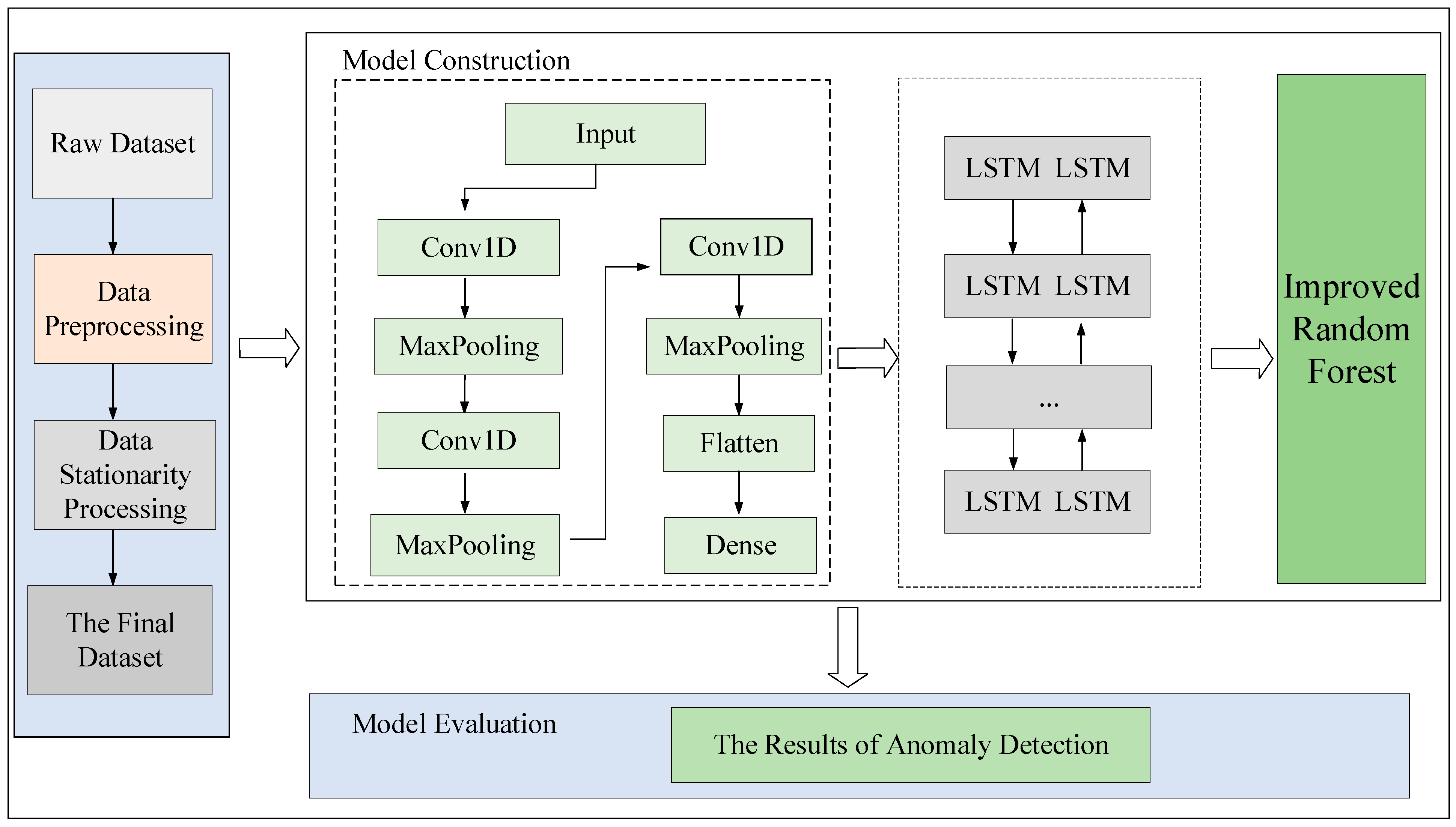
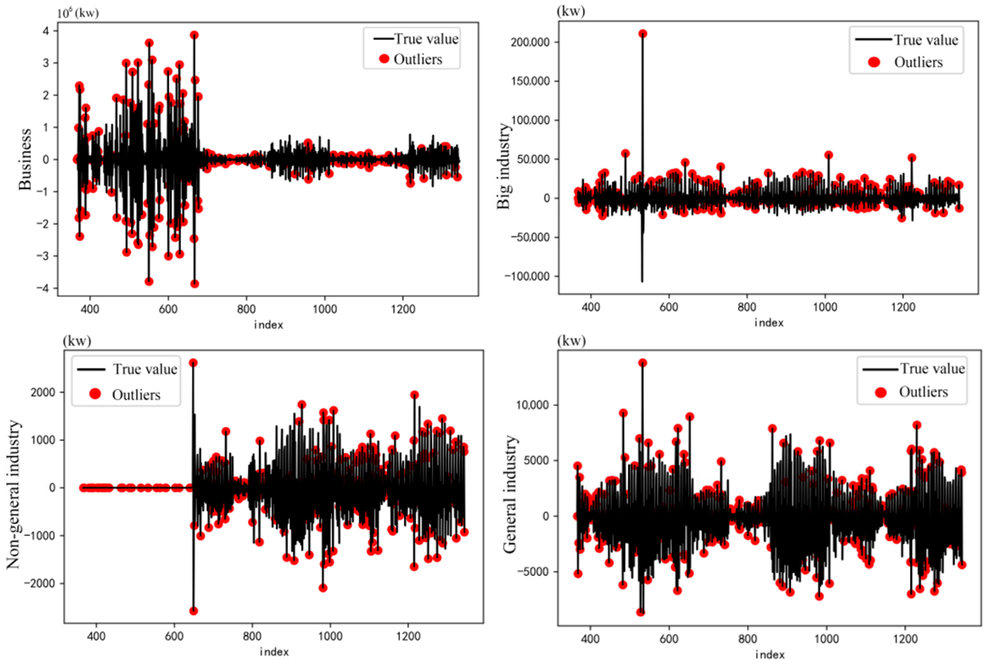
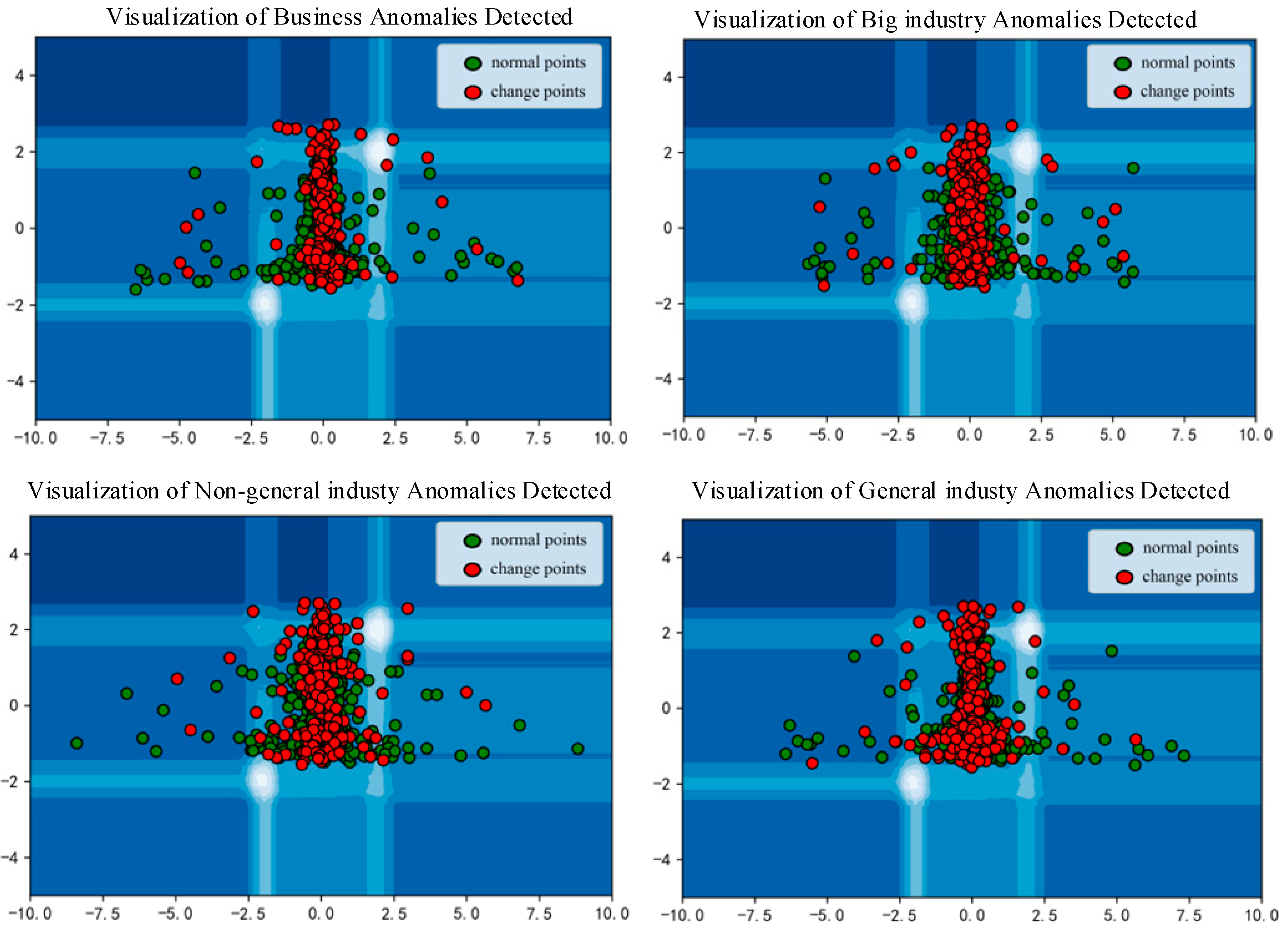
We first conducted anomaly detection on the data to prioritize essential features during the initial training. Using the CNN-BiLSTM-RF model, we detected anomalies across four major industries: commercial, large industrial, non-general industrial, and general industrial. The parameter settings for the CNN-BiLSTM-RF model are detailed in

Table 1. CNN-BiLSTM-RF neural network model parameter settings.

Parameters	Value
Hidden layers in CNN	3
Filtters	64
Channels	3
Active function	ReLU
Units in LSTM	100
Learning-rate	0.001
Dropout	0.2

. We then applied the 3Sigma rule, identifying data points that deviated by more than three times the historical data standard deviation as abnormal. Finally, we pinpointed change points by intersecting results from the two methods, as illustrated in Figure 5. This visualization depicts the anomalies detected across the four major industries, further detailed in Figure 6.

The change points represent the difference between the current change points and the load from the previous moment. These change points and their amplitudes are indicated in the series of daily maximum loads, as depicted in Figure 5, where the red points denote the identified change points. Based on the data in Figure 6, one can observe that within the series of daily maximum loads, the business sector exhibits the largest change amplitude at 4 × 10⁶. In contrast, the industrial non-ordinary industry has the smallest amplitude, registering only at 2 × 10³.

We use weather changes as the explanatory variable, denoting ‘unchanged’ as 0 and ‘changed’ as 1. Logistic regression (LR) is a regression method that employs maximum likelihood estimation to address problems wherein the explanatory variable is categorical:

$$y=\frac{1}{1+e^{-({\omega }^{T}x+b)}}$$

(37)

Table 2. Results of logistic regression of panel data for different industry load change.

	Industry	Business	Big Industry	Non-General Industry	General Industry
Variables
Maximum temperature		−0.00751	0.0279	0.0978	0.0835
		(0.0756)	(0.0746)	(0.0793)	(0.0889)
Minimum temperature		−0.0748	−0.106	−0.233 **	−0.345 ***
		(0.0850)	(0.0806)	(0.0921)	(0.108)
Daytime wind direction		0.0958	−0.0900	0.0848	0.0584
		(0.153)	(0.115)	(0.154)	(0.158)
Start_weather		−0.107 **	−0.00316	0.00849	−0.00196
		(0.0476)	(0.0495)	(0.0497)	(0.0477)
End_weather		0.0216	0.0987 *	−0.0525	−0.0663
		(0.0482)	(0.0575)	(0.0497)	(0.0477)
Constant		4.927 ***	3.950 ***	5.129 ***	8.500 ***
		(0.914)	(0.873)	(0.951)	(1.360)

Standard errors in parentheses, *** p < 0.01, ** p < 0.05, * p < 0.1.

displays logistic regression results for the change-driving factors of key indicators across four primary industrial categories: business, big industry, non-general industry, and general industry. The first row represents the regression coefficient for each feature indicator, while the second row shows the standard error value.

From the logistic regression results presented in Table 2 for the panel data, it is evident that the factors influencing sudden load changes differ across industries. Start_weather has the most significant influence in the business sector, whereas in the big industry sector, end_weather plays a more crucial role. The minimum temperature predominantly influences both the non-general and general industries.

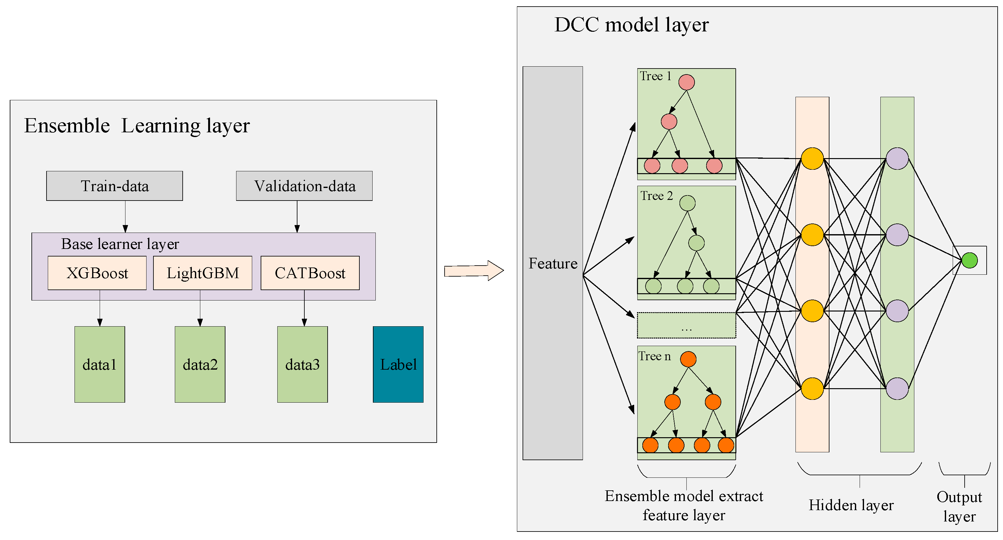
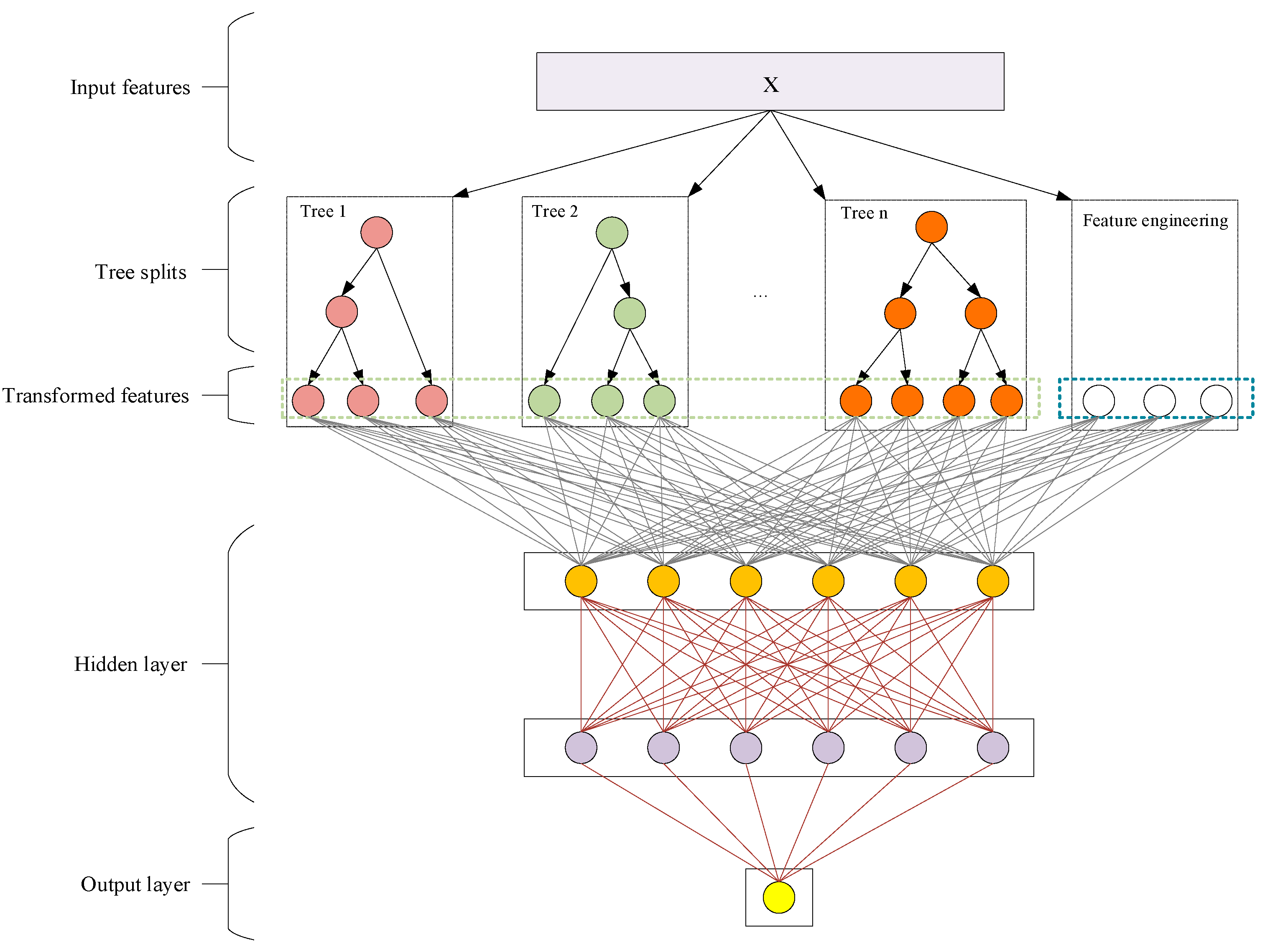
Upon ranking the features based on their significance, those of greater importance are assigned higher weights, while those of lesser significance receive lower weights. These features and their designated weights are subsequently inputted into the DCC-EL model to predict future power load values. The DCC-EL model incorporates these feature weights during its prediction process.

Table 3. DCC-EL model parameter settings.

Parameters	Value
Filtters	32
Kernel_size	3
Dilation_rate	2
Batch_size	32
Active function	Relu
Learning-rate	0.005
Dropout	0.2

details the parameter settings for the DCC-EL model.

The proposed DCC-EL model’s prediction results are compared to existing integrated learning methods. The performance of the model predictions is measured using error metrics, including mean square error (MSE), root mean square error (RMSE), mean absolute error (MAE), and mean fundamental percentage error (MAPE). The calculation methods for these four evaluation metrics are provided in Equations (38)–(41):

$$\mathrm{MSE}=\frac{1}{n}{\displaystyle \sum _{i=1}^n(}{\widehat{y}}_i-y_i{)}^2$$

(38)

$$\mathrm{RMSE}=\sqrt{\frac{1}{n}{\displaystyle \sum _{i=1}^n}({\widehat{y}}_i-y_i{)}^2}$$

(39)

$$\mathrm{MAE}=\frac{1}{n}{\displaystyle \sum _{i=1}^n|{\widehat{y}}_i-y_i|}$$

(40)

$$\mathrm{MAPE}=\frac{100\%}{n}{\displaystyle \sum _{i=1}^n|\frac{{\widehat{y}}_i-y_i}{y_i}}|$$

(41)

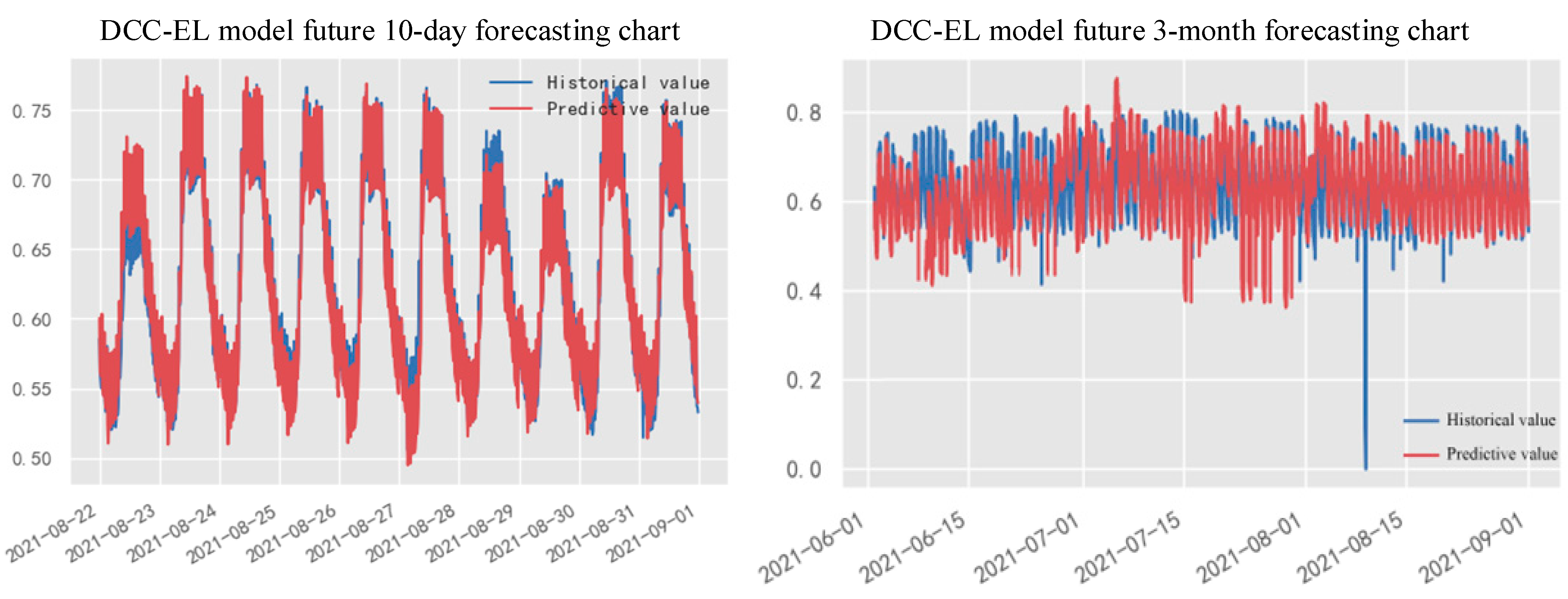
The normalized power load data were input into the DCC-EL framework for prediction, and the experimental results are illustrated in Figure 7. These charts display the power load prediction results for time intervals of ten days and three months, respectively. The horizontal axis indicates dates, while the vertical axis represents the normalized power load data. The red line depicts the predicted values derived from the DCC-EL framework, and the blue line showcases the actual power load values. For the ten-day prediction, the visual representation of the predicted values aligns closely with the actual values. However, in the three-month forecast, some variances are noticeable between the predicted and actual values. This discrepancy arises from the time sensitivity of the DCC-EL framework in mid-term load forecasting, which occasionally results in instability. Therefore, it necessitates periodic model adjustments to accommodate data fluctuations.

Table 4. Accuracy of electricity load forecast by models for the next ten days.

Model	MSE	RMSE	MAE	MAPE
Tasarruf [10]	0.0291	0.1707	0.1242	13.2469
Wu [11]	0.033	0.1817	0.062	13.1549
Veeramsetty [14]	0.0355	0.1884	0.07	14.6417
Zhang [15]	0.027	0.1643	0.054	11.0954
Fang [16]	0.0255	0.1597	0.045	8.1457
DCC	0.0347	0.1863	0.0315	16.1546
DCC-EL	0.0121	0.1101	0.0206	7.9724

and

Table 5. Accuracy of electricity load forecast by models for the next three months.

Model	MSE	RMSE	MAE	MAPE
Tasarruf [10]	0.7118	0.8443	0.6701	21.6826
Wu [11]	0.7687	0.8763	0.6595	25.8729
Veeramsetty [14]	0.7856	0.8862	0.7015	28.9389
Zhang [15]	0.689	0.8116	0.6073	24.6917
Fang [16]	0.6552	0.8093	0.6073	20.1958
DCC	0.9482	0.9738	0.5494	28.1497
DCC-EL	0.5321	0.7295	0.3567	18.4589

present the error measurements for power load predictions across six models compared to our proposed framework for time intervals of ten days and three months, respectively. Notably, the DCC model represents the dilated causal convolutional model that has not undergone feature extraction or secondary integration by the ensemble model, explicitly used for ablation studies. The other five models, referenced in the related work section of this paper, serve as benchmarks for our control experiments. Table 4 illustrates that the proposed method reduced RMSE by 4.96% and MAPE by 17.33% compared to the best results of the five models mentioned in the introduction. Table 5 illustrates that the proposed method realized a 12.31% reduction in MSE for three-month interval predictions, and the power load predictions using the DCC-EL framework generally outperform the five models.

The analysis of the control experiment results is as follows:

(1) Compared with Tasarruf’s model [10] in a control experiment, the DCC-EL model proposed in this study reduced the RMSE and MSE for predicting power loads over ten days and three months by 6.06% and 17.97%, respectively. The discrepancy in the experimental results might arise from the process of model integration, especially transitioning from Prophet to LSTM and then to BPNN. The handling and transformation of data during these stages could lead to loss or distortion of information. Such a loss can stem from various factors. For instance, each model may interpret data differently and assign varying weights to them. Minor inconsistencies might also emerge during the data conversion process between models. More critically, for such a model setup, if the outputs from the different models are not appropriately amalgamated or aligned, it could adversely impact the final prediction, especially when significant differences exist between these outputs.

(2) Compared with Wu’s model [11] in a control experiment, the DCC-EL model reduced the RMSE and MSE for predicting power loads over ten days and three months by 7.16% and 23.66%, respectively. The reason for the discrepancies in the experimental results may be that the combination of multiple models makes the debugging of the model more complicated. When there are issues with the model or its predictive performance is unsatisfactory, it is challenging to determine which part is problematic, increasing the difficulty of debugging. The complex relationships between the various models might also result in the model performing well on the training data but poorly on unseen data. Hence, this combination of models might elevate the risk of overfitting.

(3) Compared with Veeramsetty’s model [14] in a control experiment, the DCC-EL model reduced the RMSE and MSE for predicting power loads over ten days and three months by 7.83% and 25.35%, respectively. The reasons for the discrepancies in the experimental results may be that while RF can assign importance to features, if the GRU relies heavily on certain features, simply reducing dimensions using RF might result in the loss of crucial information. Additionally, with new data, while random forest might adapt quickly, the GRU might require retraining, potentially leading to challenges in updating the model.

(4) Compared with Zhang’s model [15] in a control experiment, the DCC-EL model reduced the RMSE and MSE for predicting power loads over ten days and three months by 5.42% and 15.69%, respectively. The reasons for the discrepancies in the experimental results may be as follows: first, the data may need appropriate preprocessing to fit the input requirements of VMD, LSTM, and LightGBM, which could complicate implementation. Similarly, the outputs might require proper post-processing for integration and interpretation. Moreover, using VMD for feature decomposition could introduce additional uncertainties, and the model’s stability might be affected by various model integration methods.

(5) Compared with Fang’s model [16] in a control experiment, the DCC-EL model reduced the RMSE and MSE for predicting power loads over ten days and three months by 4.96% and 12.31%, respectively. The reasons for the discrepancies in the experimental results may be: Firstly, ensemble empirical mode decomposition requires appropriate parameter settings and technical expertise for the comparison model. Otherwise, it may lead to inaccurate decomposition of high and low frequencies. Secondly, the low-frequency part might encompass nonlinear changes caused by long-term trends, periodicity, seasonality, or other intricate factors. Employing multivariate linear regression might fall short of capturing such nonlinear relationships or more complicated patterns. If these nonlinear relationships or patterns are crucial in the low-frequency section, relying solely on multivariate linear regression could result in predictive errors.

(6) The ablation experiment for DCC in the DCC-EL model showed that the performance of the DCC-EL model is far superior to that of the DCC model. This is because the DCC-EL model adopts an ensemble learning strategy, combining multiple base learners, allowing it to better integrate the characteristics and advantages of different models. This enables DCC-EL to learn a richer feature representation and better capture the complex relationships in the data, thereby improving predictive performance. Furthermore, during the prediction process, the DCC-EL model considers the weight of features, assigning weights to them based on their importance, making the model pay more attention to features that significantly impact the prediction results. This helps reduce the interference of unimportant features on prediction, enhancing the model’s stability and accuracy.

When using the proposed DCC-EL framework for power load prediction, the results surpassed those of the other six models across nearly all four evaluation metrics (MSE, RMSE, MAE, and MAPE), underscoring the efficacy of the DCC-EL framework.

4. Conclusions and Future Work

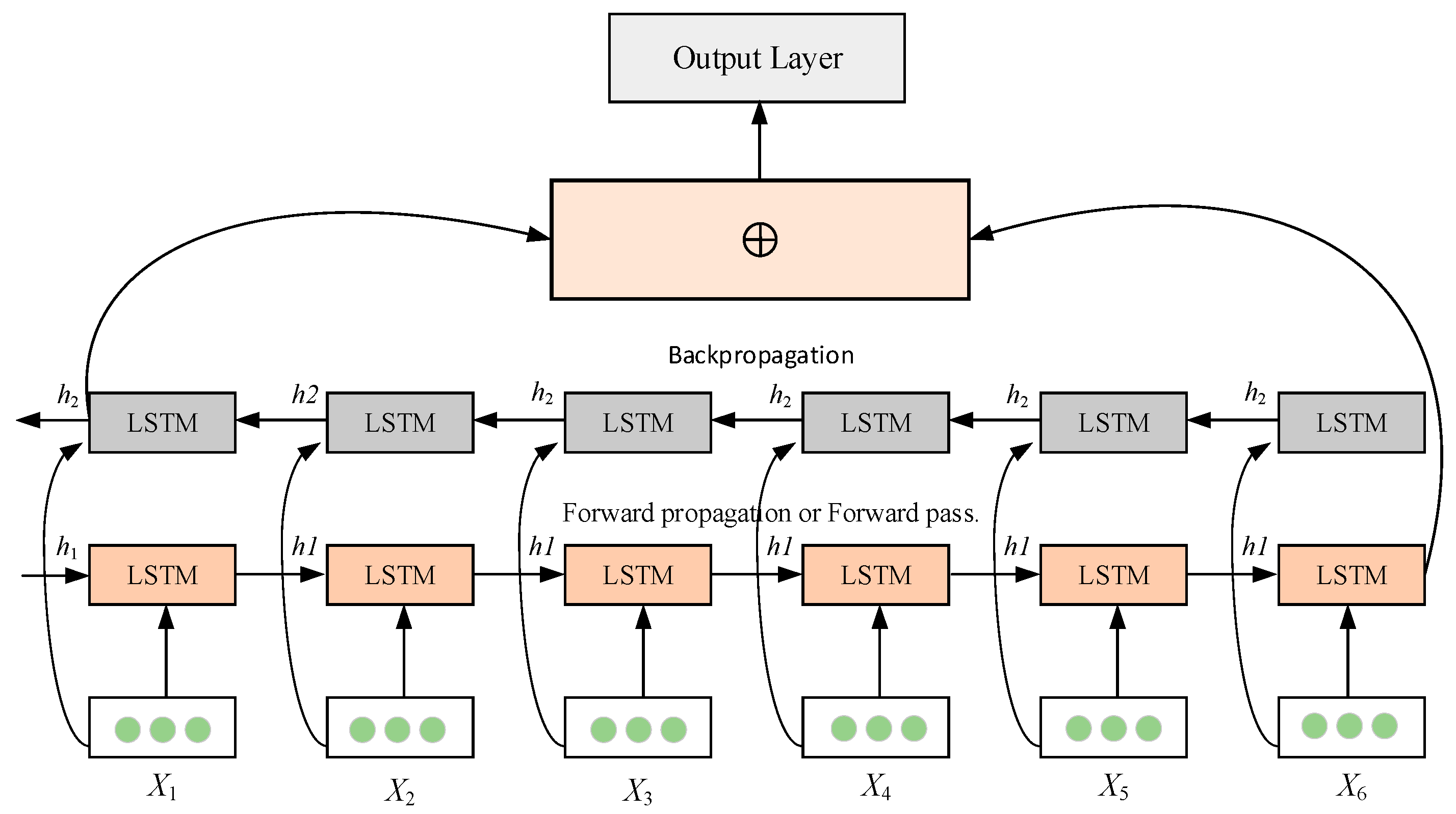
In summary, this paper introduces an innovative hybrid framework, namely CNN-BiLSTM-RF and DCC-EL, for anomaly detection in electricity load and short-to-mid-term electricity load forecasting. The proposed framework integrates the advantages of deep learning and ensemble learning. It employs CNN for feature extraction, BiLSTM to capture temporal dependencies, and improved RF for classification during the anomaly detection phase. Subsequently, the DCC-EL model is utilized to forecast future electricity load values, leveraging features extracted by the ensemble learning model.

Experimental results indicate that compared to existing models, its RMSE and MSE in short-term and mid-term electricity load forecasting are reduced by 4.96% and 12.31%. This demonstrates that our model can more accurately capture and predict the complex patterns within electricity load data, providing a reliable foundation for energy management and grid planning.

However, like any model, ours also has limitations and potential areas for improvement. Future work will focus on applying this framework to more intricate electricity load-forecasting scenarios, exploring its robustness, and enhancing prediction accuracy by integrating more advanced technologies. We also anticipate developing strategies that allow our model to adapt to data changes over time, further improving its forecasting performance.

References

1. Xian, H.; Che, J. Multi-space collaboration framework based optimal model selection for power load forecasting. Appl. Energy 2022, 314, 118937. [Google Scholar] [CrossRef]
2. Kan, Y.Z.; Sun, D.Y.; Luo, Y.; Qin, D.; Shi, J.; Ma, K. Optimal design of the gear ratio of a power reflux hydraulic transmission system based on data mining. Mech. Mach. Theory 2019, 142, 103600. [Google Scholar] [CrossRef]
3. Barocio, E.; Korba, P.; Sattinger, W.; Segundo Sevilla, F.R. Online coherency identification and stability condition for large interconnected power systems using an unsupervised data mining technique. IET Gener. Transm. Distrib. 2019, 13, 3323–3333. [Google Scholar] [CrossRef]
4. Gong, F.; Gong, T.; Yu, Y.; Sheng, Y.; Liu, K.; Kong, X. An Electricity Load Forecasting Algorithm Based on Kernel Lasso Regression. In Proceedings of the 2021 IEEE 4th International Electrical and Energy Conference (CIEEC), Wuhan, China, 28–30 May 2021; pp. 1–4. [Google Scholar]
5. Wang, Z.; Zhou, X.; Tian, J.; Huang, T. Hierarchical parameter optimization based support vector regression for power load forecasting. Sustain. Cities Soc. 2021, 71, 102937. [Google Scholar] [CrossRef]
6. Chodakowska, E.; Nazarko, J. Nazarko, ARIMA Models in Electrical Load Forecasting and Their Robustness to Noise. Energies 2021, 14, 7952. [Google Scholar] [CrossRef]
7. Yan, K.; Wang, X.; Du, Y.; Jin, N.; Huang, H.; Zhou, H. Multi-Step Short-Term Power Consumption Forecasting with a Hybrid Deep Learning Strategy. Energies 2018, 11, 3089. [Google Scholar] [CrossRef]
8. Ke, L.; Guo, W.; Shen, X.; Tan, Z. Research on the Forecast Model of Electricity Power Industry Loan Based on GA-BP Neural Network. Int. Conf. Adv. Energy Eng. 2012, 14, 1918–1924. [Google Scholar] [CrossRef]
9. Xia, T.; Zhou, Y.; Zhan, S.; Lin, H.; Zhang, T.; Lan, Y. Research on short-term load forecasting of power system based on gradient lifting tree. Int. J. Power Energy Convers. 2022, 13, 235–247. [Google Scholar] [CrossRef]
10. Tasarruf, B.; Chen, H.; Muhammad, F.; Zhu, L. Short term electricity load forecasting using hybrid prophet-LSTM model optimized by BPNN. Energy Rep. 2022, 8, 1678–1686. [Google Scholar]
11. Wu, K.; Wu, J.; Feng, L.; Yang, B.; Liang, R.; Yang, S.; Zhao, R. An attention-based CNN-LSTM-BiLSTM model for short-term electric load forecasting in integrated energy system. Int. Trans. Electr. Energy Syst. 2021, 31, e12637. [Google Scholar] [CrossRef]
12. Aguilar Madrid, E.; Antonio, N. Short-Term Electricity Load Forecasting with Machine Learning. Information 2021, 12, 50. [Google Scholar] [CrossRef]
13. Lin, J.; Ma, J.; Zhu, J.; Cui, Y. Short-term load forecasting based on LSTM networks considering attention mechanism. Int. J. Electr. Power Energy Syst. 2022, 137, 107818. [Google Scholar] [CrossRef]
14. Veeramsetty, V.; Reddy, K.R.; Santhosh, M.; Mohnot, A.; Singal, G. Short-term electric power load forecasting using random forest and gated recurrent unit. Electr. Eng. 2022, 104, 307–329. [Google Scholar] [CrossRef]
15. Zhang, W.; Yu, C.; Wang, S.; Li, T.; He, T.; He, X.; Chen, J. Short-term power load forecasting based on VMD-LSTM-LightGBM with multi-feature integration. South. Power Grid Technol. 2023, 17, 74–81. [Google Scholar]
16. Fang, N.; Li, J.; Chen, H.; Li, X. Short-term power load forecasting based on CNN-GRU-MLR with multi-frequency combination. Comput. Simul. 2023, 40, 118–124. [Google Scholar]
17. Li, C.; Chen, Z.; Liu, J.; Li, D.; Gao, X.; Di, F.; Li, L.; Ji, X. Power Load Forecasting Based on the Combined Model of LSTM and XGBoost. In Proceedings of the 2019 the International Conference on Pattern Recognition and Artificial Intelligence (PRAI’19). Association for Computing Machinery, Wenzhou, China, 26–28 August 2019; pp. 46–51. [Google Scholar]
18. Wang, Z.; Shao, E.; Wang, C. Conv-AdaRNN: A Power Load Forecasting Method Based on CNN and AdaRNN. In Proceedings of the 2022 5th International Conference on Hot Information-Centric Networking (HotICN), Guangzhou, China, 24–26 November 2022; pp. 72–76. [Google Scholar]
19. Zhou, Q.; Zhu, Z.; Xian, G.; Li, C. A novel regression method for harmonic analysis of time series. ISPRS J. Photogramm. Remote Sens. 2022, 185, 48–61. [Google Scholar] [CrossRef]
20. Kohavi, R. A study of cross-validation and bootstrap for accuracy estimation and model selection. In International Joint Conference on Artificial Intelligence; Morgan Kaufmann Publishers Inc.: Burlington, MA, USA, 1995. [Google Scholar]
21. Hu, L.; Wang, J.; Guo, Z.; Zheng, T. Load Forecasting Based on LVMD-DBFCM Load Curve Clustering and the CNN-IVIA-BLSTM Model. Appl. Sci. 2023, 13, 7332. [Google Scholar] [CrossRef]
22. Le, C.; Bengio, Y.; Hinton, G. Deep learning. Nature 2015, 521, 436–444. [Google Scholar]
23. Dogan, Y. A New Global Pooling Method for Deep Neural Networks: Global Average of Top-K Max-Pooling. Trait. Signal 2023, 40, 577–587. [Google Scholar] [CrossRef]
24. Siami-Namini, S.; Tavakoli, N.; Namin, A.S. The performance of LSTM and BiLSTM in forecasting time series. In Proceedings of the 2019 IEEE International Conference on Big Data (Big Data), Los Angeles, CA, USA, 9–12 December 2019; IEEE: Piscataway, NJ, USA, 2019; pp. 3285–3292. [Google Scholar]
25. Breiman, L. Random Forests. Mach. Learn. 2001, 45, 5–32. [Google Scholar] [CrossRef]
26. Speiser, J.L.; Miller, M.E.; Tooze, J.; Ip, E. A comparison of random forest variable selection methods for classification prediction modeling. Expert Syst. Appl. 2019, 134, 93–101. [Google Scholar] [CrossRef] [PubMed]
27. Paul, A.; Mukherjee, D.P.; Das, P.; Gangopadhyay, A.; Chintha, A.R.; Kundu, S. Improved Random Forest for Classification. IEEE Trans. Image Process. 2018, 27, 4012–4024. [Google Scholar] [CrossRef]
28. Chaudhary, A.; Kolhe, S.; Kamal, R. An improved random forest classifier for multi-class classification. Inf. Process. Agric. 2016, 3, 215–222. [Google Scholar] [CrossRef]
29. Li, X.N.; Yu, Q.; Yang, Y.; Tang, C.; Wang, J. An evolutionary ensemble model based on GA for epidemic transmission prediction. J. Intell. Fuzzy Syst. 2023, 44, 7469–7481. [Google Scholar] [CrossRef]
30. Dong, X.; Yu, Z.; Cao, W.; Shi, Y.; Ma, Q. A survey on ensemble learning. Front. Comput. Sci. 2020, 14, 241–258. [Google Scholar] [CrossRef]
31. Cho, J.; Yoon, Y.; Son, Y.; Kim, H.; Ryu, H.; Jang, G. A Study on Load Forecasting of Distribution Line Based on Ensemble Learning for Mid- to Long-Term Distribution Planning. Energies 2022, 15, 2987. [Google Scholar] [CrossRef]
32. Schapire, R.E.; Singer, Y. Improved boosting algorithms using confidence-rated predictions. Mach. Learn. 1999, 37, 297–336. [Google Scholar] [CrossRef]
33. Bai, S.; Kolter, J.Z.; Koltun, V. An empirical evaluation of generic convolutional and recurrent networks for sequence modeling. arXiv 2018, arXiv:1803.01271. [Google Scholar]
34. Yang, Y.; Gu, Z.H. Medium-term power load forecasting based on XGBOOST-DNN. Comput. Syst. Appl. 2021, 30, 186–191. [Google Scholar]
Figure 1. The structure diagram of the CNN-BiLSTM-RF method.
Applsci 13 09706 g001
Figure 2. Bi-LSTM architecture diagram.
Applsci 13 09706 g002
Figure 3. DCC-EL forecasting framework.
Applsci 13 09706 g003
Figure 4. Details of dilated causal convolutional neural network.
Applsci 13 09706 g004
Figure 5. Visualization of the four major industries’ anomalies detected.
Applsci 13 09706 g005
Figure 6. Visualization of the four major industries’ anomalies detected by 3Sigma rule.
Applsci 13 09706 g006
Figure 7. DCC-EL model future ten-day and three-month forecasting chart.
Applsci 13 09706 g007