Abstract
The issue of congestion on urban roads stems from an imbalance between transport demand and supply. It has become imperative to address the problem from the traffic demand side. While managing effective traffic demand relies on understanding the individual preferences of drivers, the current method for gathering preferences (i.e., through questionnaires) is both expensive and may not accurately capture the characteristics of respondents due to their varying interpretations of the options. To overcome these challenges, we proposed a path recommendation method that takes individual travel preferences into consideration by employing automatic license plate recognition (ALPR) data for the extraction of individual travel preferences. We initially identified key factors influencing the path selection behaviors of drivers, including path attributes, travel attributes, and individual attributes. Subsequently, we constructed a path satisfaction model based on individual preferences, employing an improved analytic hierarchy process (AHP). Furthermore, we utilized the pth percentile approach, rather than expert scores, in order to determine the relative importance of each indicator in the improved AHP. By applying the proposed model to the ALPR data from Xuancheng City, we successfully extracted the path selection preferences of drivers. We designed various scenarios to verify the reliability of the model, and the experimental results demonstrated that the proposed path satisfaction model can effectively capture the influence of underlying indicators on the path selection behavior of individuals with diverse travel preferences, considering different driver types and path attributes. Moreover, compared to the real trajectory, the recommended paths yielded an overall satisfaction improvement of over 10%, confirming the reliability and practicality of our proposed model.
1. Introduction
In recent years, China witnessed rapid urbanization, leading to the expansion of urban areas and significant advancements in urban road construction. However, the increasing number of motor vehicles outpaced the provision of urban road infrastructure, resulting in severe traffic congestion issues [1]. For instance, in Guangzhou, the number of motor vehicles reached 3.309 million (increased by 7.4%) in 2021 [2]; however, the total road length in the city was 11,464 km, which only increased by 31 km (or 0.3%) [3]. The fundamental problem underlying traffic congestion is the mismatch between traffic supply and demand, in terms of both time and space. Therefore, to address traffic congestion, it is necessary to consider solutions from both the supply [4,5] and demand sides [6,7]. While increasing the traffic supply can be achieved through expanding the length and density of roads, it cannot provide immediate relief. Furthermore, such measures are constrained by the urban layout, traffic structure, and land uses. Therefore, at present, managing traffic demand is crucial for tackling urban congestion. One key aspect in this line is providing personalized path recommendations that cater to individual travel preferences, which can play a pivotal role in balancing the spatial and temporal distribution of travel demand, thereby enhancing traveler satisfaction, enriching ways of traffic management, alleviating traffic congestion, and improving urban traffic efficiency.
Previous studies on personalized path recommendations for drivers considered various factors. Traditional studies considered optimization objectives such as the shortest path, shortest travel time, or lowest fuel consumption, and utilized algorithms such as Dijkstra’s algorithm [8] or the A* algorithm [9]. Subsequent studies incorporated time-varying characteristics of the traffic system, proposing dynamic path planning methods which are applicable to changing road network environments [10]. Other research focused on the selection of parking lots as part of the path recommendation process, constructing two-layer planning models that incorporate the length of the path from the starting point and end point to the parking lot [11]. Additionally, some studies analyzed the behavioral habits of drivers—such as braking, acceleration, and steering—by utilizing onboard vehicle operation sensors, in order to recommend optimal paths in alignment with the driver’s habits [12].
While these studies discussed factors influencing path choice from different perspectives and constructed models to describe these objective factors, subjective variations exist among drivers, even under the same objective conditions. Therefore, it is necessary to construct a model that captures the subjective preferences of drivers accurately and reconstructs the decision-making process accordingly. Previous research, rooted in expected utility theory, assumed that drivers possess all relevant information and made optimal choices. However, in reality, people cannot obtain all the relevant information and tend to make instantaneous decisions. To address this, random utility theory was developed, incorporating a random error term into the expected utility to simulate human cognitive behavior. Based on this theory, an improved logit model was introduced to analyze driver’s path choice characteristics under different preferences [13]. Additionally, recognizing the bounded rationality of decision making, some researchers utilized prospect theory and cumulative prospect theory from the field of psychology to describe the limited rationality in decision-making processes [14]. Based on prospect theory, scholars such as Zhang et al. [15] and Ghader [16] incorporated risk preference factors and road network familiarity into path choice behavior models, in order to provide recommendations to travelers.
Regarding the data used in path choice behavior research, two main types have been considered [17]. Active data collection methods include stated preference (SP) surveys and revealed preference (RP) surveys, while passive data comprises GPS data, automatic license plate recognition (ALPR) data, and other sources that capture the travel trajectories of travelers. For example, Humagain [18] collected data on ideal and actual commuting times through questionnaire surveys issued to commuters, allowing for exploration of the factors influencing their commuting time satisfaction. Liu et al. [19] collected data on individual attributes, information preferences, and path choice preferences through RP surveys, then analyzed the influence of individual attributes and information type preferences on the commuter path choice using structural equation modeling. Correa et al. [20] compared user travel paths between origin–destination (OD) pairs considering the K-shortest paths, using GPS data to explore the relationship between traveler path choice behavior and general traffic conditions. While active data obtained through questionnaires can target the specific information needed for research, they suffer from small sample sizes, high acquisition costs, and potential biases due to respondents misunderstanding the options.
According to the analysis above, personalized path recommendation research emphasizes the comprehensive extraction of individual preferences, accurate description of path choice behavior, and analysis of the interactions between influencing factors. However, there is still a need for further research on the use of passive data collection techniques, such as ALPR data, for the extraction of individual preferences and construction of path selection models.
To maximize the information available in ALPR data and reduce the cost of acquiring individual preferences, we proposed a method that utilizes such data to extract individual travel preferences and recommend paths accordingly. The structure of this article is shown in Figure 1. Firstly, we analyzed the influence of the path, traffic conditions, and individual factors on driver path selection behavior, providing calculation methods for each influencing factor based on ALPR data. Secondly, the traditional AHP was improved by determining the importance of each indicator using the pth percentile importance score. Finally, by combining the path satisfaction calculation method with path attributes and individual preferences, personalized path recommendations can be made for travelers.
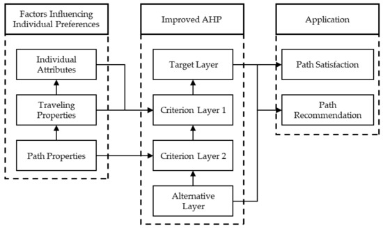
Figure 1.
Structure of the article.
The main contributions of this paper are as follows:
- A path satisfaction calculation method based on ALPR data was proposed based on ALPR data. By analyzing the trajectory data obtained through ALPR data, the driver type was identified and their path selection preferences were extracted. This approach makes the quantification of individual preferences at low cost, providing a new avenue for quantifying preferences using ALPR data.
- An indicator importance scoring method was proposed. We suggested using the pth percentile method to evaluate the importance of the indicators instead of relying on expert evaluations which are used in traditional AHP. This approach enhanced objectivity and stability in the construction of the comparison matrix, thus improving the accuracy of the model.
- To validate the effectiveness of the proposed method, we designed and conducted experiments, and the results demonstrated the efficacy and superiority of the proposed method in capturing individual preferences and generating personalized path recommendations.
2. Factors Influencing Individual Preferences
2.1. Path Properties
In this paper, we recognized that both the physical characteristics of a path and the traffic conditions along the path play crucial roles in influencing a driver’s travel experience. As a result, these factors significantly impact the driver’s choice of a path. To investigate this relationship, we utilized ALPR data as the basis for our analysis. We carefully selected relevant attributes that represent both the static features of paths and the dynamic attributes associated with traffic conditions for our research. By considering these representative attributes, we aimed to gain a comprehensive understanding of how these factors shape the preferences of drivers when selecting their travel paths.
Before introducing the properties, we defined path as a sequence of road segments from the origin to the destination. Thus, the path can be expressed as follows: , where represents a road segment.
2.1.1. Static Properties
Various static attributes of paths were considered, in order to understand their impact on driver path choice [12,21,22]. These static attributes include:
- 1.
- Path length
This attribute represents the total distance of the roads that a driver travels from origin to destination. Shorter paths are generally preferred by drivers, as they intuitively reflect lower travel costs. The path length is calculated by summing the lengths of road segments:
where represents the length of the road .
- 2.
- Number of path lanes
This attribute reflects the overall number of lanes on a path. It is calculated as the weighted average of the number of lanes on each road segment, considering their respective lengths. Drivers tend to choose paths with more lanes, which are generally indicative of higher road levels or capacities. The number of lanes in the path, is calculated as follows:
where represents number of lanes in the road .
- 3.
- Number of path intersections
This attribute measures the total number of intersections present along a path. It provides an indication of the potential risk of delays during the trip. Drivers generally prefer paths with fewer intersections, as this can minimize their chances of being affected by signal control and experiencing travel-time delays. The number of intersections in a path consists of road segments, , is calculated as:
- 4.
- Path turning index
This attribute takes into account the number and directions of turns along the path. It reflects the driver’s turning actions and measures the ease of driving along the path. Different turning operations require varying levels of attention from drivers, with U-turns typically being the most challenging and straight movements being the easiest. Drivers tend to choose paths with smaller path turning index to complete their trips. The path turning index, , is calculated as:
where represents the turning value for direction of road towards the next road , which is calculated as follows:
In other words, the turning value is assigned as follows: 1 for straight ahead, 2 for a right turn, 3 for a left turn, and 4 for a U-turn. In this paper, the turns were calculated based on the road network information. They were recorded as and , where represents the north deviation angle between the direction of traffic and the north direction (clockwise direction is positive) when entering the intersection or exiting the road, while represents the north deviation angle when entering the road or exiting the intersection. The north deviation angle falls within the value range of . The upstream section, denoted by , represents the direction of travel from into the intersection. On the other hand, represents the direction of travel from the intersection into the downstream . The turning angle, denoted as , is calculated as follows:
The turning is determined based on the turning angle. An angle of 0° corresponds to straight driving, 90° to a right turn, 180° to a U-turn, and 270° to a left turn. However, in reality, urban road networks often have angles between road that do not strictly align with these values. Therefore, it is necessary to adjust the angle restrictions. A related study [23] suggested that urban roads tend to connect at angles less than 30°. It can be assumed that drivers do not exert extra effort within this angle range. Hence, the floating range for straight driving and U-turns was increased by 30°. Similar adjustments were made for left and right turns, accordingly. Thus, the calculation method for the steering when driving from road section to road section is as follows:
Take Figure 2 as an example. Assuming that each road segment in the path has a length of one unit and that the number of lanes on each road is 2, 2, 3, and 3, respectively, according to Equations (1)–(7), the length of the path is 4, the number of path lanes is 2.5, the number of path intersections is 0.75, and the path turning factor is 1.5.
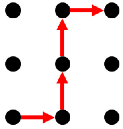
Figure 2.
Schematic diagram of the path.
2.1.2. Dynamic Properties
The traffic state attributes include the dynamic and potentially time-varying characteristics of a path that influence the selection of a path by a driver. These attributes include path travel time, as well as maximum and average path density [21,22].
- 1.
- Path Travel Time
Traditionally, path travel time and path length serve as optimization objectives in relevant research. Path travel time is a crucial indicator that reflects the overall travel conditions and results from the interplay of various traffic factors.
- 2.
- Maximum and Average Path Density
In addition to considering path travel time, drivers also take into account the traffic state along a path when making path choices. A favorable traffic state is more likely to be selected by drivers. Moreover, the path density, which characterizes the traffic state, can impact the comfort level of travelers. Drivers prefer paths with smaller maximum and average path densities. The average path density, denoted as , can be calculated as follows:
where is density of at a specific time window, which is calculated as follows:
where is total time cost of all cars passed during a time window of (5 min).
The maximum path density, denoted as , is calculated as follows:
2.2. Traveling Properties
Traveling attributes [24], including the travel purpose, expected duration, and frequency, play a significant role in shaping a driver’s travel behavior. These attributes, either independently or in combination, have an impact on path selection and the likelihood of path changes.
- 1.
- Purpose of trip and expected length of trip
The arrival time of commuting trips is typically fixed and, so, the desired travel time for these drivers is determined by the time difference between their departure time and the desired arrival time. When the expected travel time is lengthy, drivers usually opt for paths based on their regular habits. Conversely, when the expected travel time is short, they prioritize the travel time factor of the path, sometimes overlooking other relevant factors. Furthermore, when selecting paths for medical and business trips, drivers tend to plan ahead and avoid paths with high levels of uncertainty. On the other hand, drivers embarking on leisure and recreation trips do not have strict expectations regarding travel time and display a degree of spontaneity when choosing their paths.
- 2.
- Frequency of trips
The frequency of trips is indicative of a driver’s travel experience and their familiarity with the road network. Drivers who travel more frequently tend to select travel paths based on their established driving habits. Conversely, drivers who travel less frequently tend to rely on external path recommendations, as they may have limited knowledge of the road network and traffic conditions.
2.3. Individual Attributes
Individual driver attributes have a significant role in the path selection preferences of drivers. These preferences are influenced by various factors, including gender, age, driving experience, occupation, and personality. Differences in path preferences can be observed in terms of sensitivity to path travel time stability, tendency to stick to historical paths, path difficulty, and preference for traffic conditions. In this study, instead of relying on questionnaires, we utilized ALPR data to determine individual driver attributes. To quantify drivers with specific attributes, we introduced a counting function, denoted as , which calculates the number of times the condition is satisfied for all travel trajectories of the same driver under the same OD pair for seven consecutive days. Assuming that the driver associated with the same license plate number remains consistent in the detection data, we can quantify drivers based on each attribute, as follows.
- 1.
- Stability of travel time
Drivers who prioritize stable travel time have a higher demand for reliable travel time and place certain requirements on the arrival time or travel duration under the same OD pair. This preference is often observed when considering regular travel behaviors such as commuting or going to school. The identification of drivers who prioritize stable travel time is determined as follows:
where and represent the latest arrival time and maximum travel duration, respectively, for the same OD pair over seven consecutive days; and represent the arrival time and travel duration for a specific trip, respectively; and and are the respective time and count thresholds. The expression represents the count of occurrences where the time difference between the latest arrival time and the current arrival time, or the difference between the maximum travel duration and the current travel duration is less than within all travel trajectories of a driver for the same OD pair over seven consecutive days. Based on relevant research [25], the values chosen for and in this study were 15 min and 2 times, respectively. In other words, drivers who had a count greater than or equal to two for occurrences where the floating difference in arrival time or travel duration for the same OD pair over seven consecutive days was less than 15 min were considered to possess the attribute of travel time stability. The strength of this attribute is determined by the value on the left side of Equation (11).
- 2.
- Historical Inertia
Historical inertia, in the context of a driver’s path choice between OD pairs, exemplifies the stability exhibited by experienced drivers who possess a certain level of familiarity with the travel path. These seasoned drivers boast a wealth of knowledge regarding traffic information and possess a heightened sense of confidence in their own judgment. Consequently, they are less inclined to deviate from their established travel paths. A driver who would be regarded as being with historical inertia should meet the following condition:
where denotes the path with the highest number of trips for a specific driver over a 7-day period, while represents a specific trip path. Additionally, β was assigned a value of 2 in this study. It is important to note that we considered drivers as having exhibited historical inertia if they repeated the same trip path under the same OD pair at least twice within a span of seven consecutive days.
- 3.
- Path Difficulty
Path difficulty is an indicator of a driver’s preference for a comfortable path, which is primarily influenced by factors such as the path turning index, the number of path lanes, and the number of path intersections. However, when compared to historical inertia and trip time stability, path difficulty is considered a relatively minor factor. Its significance diminishes when prioritizing time stability and historical inertia. In this study, a driver’s preference for path difficulty was quantified by calculating the percentile of path ease for the driver’s travel trajectory within the target OD pair, relative to all trajectories recorded in the historical data for that OD:
where is calculated as:
where represents the percentile rank of the number of lanes the driver traverses in their travel trajectory over 7 consecutive days within the OD pair. It should be noted that, when calculating the pth percentile, the values are sorted in ascending order. Therefore, it is necessary to process such that the percentile of the number of lanes aligns with the direction of intersection indicators (here, a smaller indicates better traffic conditions). Similarly, , , and have the same interpretation. Furthermore, was set to 2, which means that, if the number of instances where the difficulty percentile of the path was less than 50 within the 7-day period at least two times, a preference for easier roads could be concluded.
- 4.
- Traffic Status
Traffic status preference reflects the degree to which drivers tolerate traffic congestion, which is influenced by the average and maximum path densities. When there is a significant change in traffic conditions, drivers with different preferences exhibit varying levels of willingness to change their paths. In the historical trajectory data, the traffic state preference of a driver is determined by calculating the percentile of the path traffic status within the travel trajectory of the target OD pair, relative to the traffic states observed in all recorded trajectories:
where represents the percentile rank of the lane density in the driver’s travel trajectory over 7 consecutive days for a specific OD pair. This determines the position of the lane density, , among all the trajectories within that OD pair. Setting β to 2 means that the driver’s chosen path had a density percentile lower than 50 on at least two instances within the 7-day period. This criterion suggests that the driver prefers paths with less traffic congestion, indicating a tendency to select paths with lower density percentiles.
3. A Path Satisfaction Model Considering Individual Preferences
In the previous section, the factors affecting path satisfaction were categorized into path-level and individual-level factors. It was observed that drivers with varying individual attributes exhibited distinct preferences for these factors, leading to variations in path satisfaction. Extracting the individual preferences of different drivers poses an evaluation challenge involving multiple levels and factors. To address this issue, we enhanced the AHP by introducing an individual preference extraction approach based on ALPR data. This method aimed to capture and analyze the unique preferences of each driver, taking into account their individual attributes, thus enabling a more comprehensive understanding of the factors influencing path satisfaction.
3.1. Hierarchical Analysis Method
The AHP [26] is a multi-criteria decision-making method proposed by Saaty, an esteemed American operations researcher. The key feature of AHP is in its ability to quantify complex and fuzzy evaluation problems. This is achieved by breaking down objectives into layers and factors, comparing and calculating these factors within the same layer. In this process, weight values are assigned to each factor, providing a quantitative basis for evaluating the overall problem and ultimately selecting the optimal solution. In practical applications, the AHP consists of four essential steps. First, a hierarchical model is constructed to capture the relationships between the evaluation object and its related indicators. Second, a comparison matrix is constructed to establish the relative importance of these indicators. Subsequently, the weight-solution and consistency test are carried out to ensure accuracy and reliability. Finally, based on the quantitative results, the optimal solution is determined.
- 1.
- Building a hierarchical model
The process of constructing a hierarchical model involves continuously deconstructing the original problem through logical analysis. This process entails breaking down the complex problem into important influencing factors, forming the next layer, and deciding whether further deconstruction is necessary based on the actual situation. By following this approach, the indicators are gradually refined according to different layers, resulting in the construction of a systematic hierarchical model, as depicted in Figure 3.
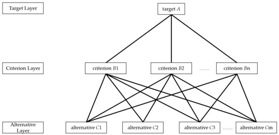
Figure 3.
Hierarchical model.
In this paper, when constructing the model for individual travel satisfaction, we ensured the systematicity and completeness of the indicator system while refining it. This process led to the identification of several bottom-layer indicators. A complex problem is typically decomposed into three layers:
The first layer is the target layer, which represents the primary objective that needs to be quantitatively described. The construction of the layer analysis model aims to determine the magnitude of each layer indicator’s impact on the target layer, quantitatively representing this impact for ease of selection or decision making.
The second layer is the criterion layer. The criterion layer represents the objectives or criteria that must be followed to solve a problem or evaluate an objective. It establishes a link to the upper layer, providing a basis for decision making, and serves as a refined indicator of the upper layer’s objective. Additionally, the criterion layer extends downward, generating more refined and detailed indicators.
The third layer is the alternative layer, which is often the bottom layer. The alternative layer comprises potential solutions related to the target layer and forms the subject of decision making in the hierarchical analysis. Indicators within the alternative layer are usually more intuitive and clear, allowing for easier quantitative analysis. This enables the qualitative judgment of the target layer to be translated into quantitative calculations.
- 2.
- Construction of comparison matrix
Hierarchical analysis facilitates the decomposition of complex problems during the model construction process. The hierarchical model comprises secondary indicators, tertiary indicators, and even more detailed sub-indicators at the fourth and fifth layers. However, it is important to note that the indicators in the same layer may not be of equal importance. When faced with multiple indicators in the upper layer, decision makers are typically tasked with determining their relative importance. This often relies on their experience, logical reasoning, and scientific judgment to assign value to different indicators, thereby transforming qualitative issues into quantitative ones.
The traditional AHP achieves this objective by employing a numerical scale ranging from 1 to 9, as illustrated in Table 1. This scale allows for clear differentiation of value judgments, where the values 1, 3, 5, 7, and 9 represent distinct levels of importance. Intermediate values (e.g., 2, 4, 6, and 8) occupy fuzzy spaces, allowing for more nuanced assessments.

Table 1.
The comparative scale values and their meanings.
The comparison matrix is constructed by conducting pairwise comparisons and assigning numerical scores to facilitate the conversion of qualitative problems into quantitative ones. For example, consider the target layer A and criterion layer B. We defined the comparison matrix as follows:
Then, the matrix satisfies the following characteristics:
where denotes the comparison outcome between the ith and the jth indicator.
Typically, each expert constructs a comparison matrix. Therefore, prior to constructing the comparison matrix, an expert questionnaire should be prepared [27], allowing the experts to score the importance of the indicators using values on a scale of 1–9, based on their comparison.
- 3.
- Weighting solution
Determine the maximum eigenvalue of matrix A and its corresponding eigenvector . Once the eigenvector W’ is obtained, its elements can be normalized to derive , representing the weight values of each criterion in the target layer A relative to the criterion layer B.
- 4.
- Consistency identification
The initial comparison values within each layer’s comparison matrix serve as the foundation for subsequent calculations in the AHP. In theory, as the number of criteria to be evaluated increases, the potential for conflicting pairwise comparison outcomes also increases. This arises because the scoring process only considers pairwise relationships between indicators and fails to capture the overall relationships among all criteria. For instance, contradictory results such as A > B, B > C, and A < C may arise. Hence, it becomes essential to conduct a consistency identification on the eigenvector. The consistency identification ensures that the results obtained through constructing the AHP and its comparison matrix are valid, provided the consistency criteria (CR < 0.1) are met. If the consistency check results do not meet the criteria, it is necessary to reconstruct the comparison matrix. The consistency check is performed using Formulas (18) and (19).
Consistency Index :
where is the maximum eigenvalue of A.
Consistency ratio :
where RI is the average random consistency index, the values for which are given in Table 2.
Table 2.
Average consistency index.
3.2. Path Satisfaction Model Based on Improved AHP Algorithm
We utilized ALPR data as the foundation for constructing the AHP in this study. This section presents the methodology for constructing the path satisfaction model, incorporating improvements to the AHP. The subsequent explanation outlines the path satisfaction model in alignment with the research objectives of this paper. Based on the analysis conducted previously, pertinent indicators were organized and a four-layer model was constructed, taking path satisfaction as the main objective. The hierarchical model is visually represented in Figure 4.
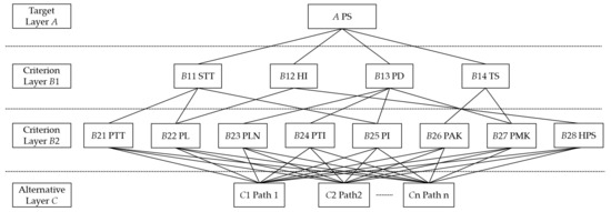
Figure 4.
Path satisfaction hierarchy model.
The path satisfaction model was structured into four layers. The target layer (A) represents path satisfaction. The criterion layer (B1) comprises individual driver attributes, including stability of travel time (STT) preference, historical inertia (HI) preference, path difficulty (PD) preference, and traffic status (TS) preference. The importance score for B1 was determined based on the corresponding characteristics in the historical trajectories of drivers. The criterion layer (B2) primarily consists of dynamic and static path attributes, such as path travel time (PTT), path length (PL), number of path lanes (PLN), path turning index (PTI), number of path intersections (PI), average path density (PAK), maximum path density (PMK), and historical path similarity (HPS). The importance score for B2 was determined by comparing the indicators for a driver’s chosen path with all trajectories within the specified time period. The alternative layer encompasses the alternative path set, comprising historical trajectories between OD pairs and several shortest paths between ODs. It is important to note that the connections in Figure 4 and the inclusion relationships in Table 3 only represent the main lower-layer indicators that influence the upper-layer indicators. During the actual calculation process, each upper-layer indicator considered all lower-layer indicators as contributing factors. The indicators without any connections had the lowest importance.
Table 3.
Main connection relationships for indicators in each layer.
To improve the objectivity in evaluating the mutual importance of indicators, we proposed an enhanced process for the construction of comparison matrices. Instead of relying on expert scoring, we utilized ALPR data as the basis for establishing a comparison matrix for each individual driver. This approach aims to simplify the construction process and make it more objective.
In the traditional AHP, the elements of the comparison matrix are assigned values on a scale of 1–9. This requires judging both the relative importance of indicators and the degree of importance, resulting in a cumbersome construction process. To address this, we simplified the elements in the comparison matrix by using three values: −1, 0, and 1. These values characterize the degree of importance among indicators. We reference the work of Li et al. [28], which inspired this simplification.
The indicators affecting the comparison matrix A included all indicators in the criterion layer B1. Thus, the comparison matrix A was a matrix:
where is determined according to the relative importance of indicator when compared to indicator . To determine the value of , we introduced an importance score :
The importance rating of each indicator is crucial, as it determines the strength of importance and the weight given by drivers to that particular factor, ultimately affecting their overall satisfaction with the chosen path. Therefore, it is essential to accurately calculate the importance rating of each indicator which, in turn, affects the accuracy of the weight values assigned to the lower-layer indicators. The calculation methods for the of the lower-layer indicators vary across different layers. The particular calculation methods are detailed below.
- 1.
- value of indicators from criterion layer B1 affecting target layer A
The indicators that were compared from criterion layer B1 were B11 STT, B12 HI, B13 PD, and B14 TS. Referring to Equations (11)–(15), the importance score for B11 temporal stability is calculated as
Similarly, the calculation methods for the importance scores , , and of B12 HI, B13 PD, and B14 TS are calculated as follows:
- 2.
- value of indicators from criterion layer B2 affecting criterion layer B1
To calculate the value for each indicator in criterion layer B2, the following indicators were considered: B21 PTT, B22 PL, B23 PLN, B24 PTI, B25 PI, B26 PAK, B27 PMK, and B28 HPS.
Using to represent the percentile value of the mean of indicator in a driver’s 7-day travel trajectories within the OD, among all the corresponding indicators of the trajectories within the same OD, the calculation method for the importance score of each indicator in criterion layer B2 is as follows:
Among the indicators B21, B22, B24, B25, B26, and B27, a higher percentile rank indicated a worse driving experience, implying a lower preference by drivers. Therefore, the percentile ranks of these indicators were utilized as their importance scores. For the indicators in criterion layer B2 that are not listed in Table 3 and which differ from the discussed indicators in criterion layer B1, their importance scores were set to 0. Subsequently, the comparison matrix was derived by determining the scale values between indicators based on Equation (21).
As an example, consider the of the indicators in criterion layer B2 to be 10, 20, 30, 40, 50, 60, 70, and 80. When calculating the comparison matrix for indicator B11, according to the table, the main connecting relationships for B11 are B21, B22, and B25. Hence, the importance scores of the remaining indicators are set to 0, resulting in the updated importance scores being 10, 20, 0, 0, 50, 0, 0, and 0. By performing further calculations using Equation (21), the comparison matrix for indicator B11 can be obtained, as follows:
- 3.
- value of indicators from alternative layer C affecting criterion layer B2
The evaluation of indicators from criterion layer B2 entails assessing the indicators associated with each path in alternative layer C. The method used to calculate the value for each path follows the same approach discussed previously and will not be repeated here. However, it is crucial to highlight that the percentile ranking of the indicators for each path, in this context, denotes the placement of those indicators relative to the corresponding indicators of all trajectories for the OD pair over a seven-day period.
The construction of the comparison matrix for each indicator in all the layers for the lower-layer indicators has been completed at this point. For the static path decision problem, the weights of all paths in the alternative path set for the target layer can be obtained, following which the path with the greatest weight can be selected as the recommended path.
However, it is important to note that the weight value obtained in this process is a relative quantity that varies with the number of alternative paths in the solution layer C. Therefore, a more stable method is required to represent the path satisfaction.
During the operation of the AHP, the weight values for indicators in any layer with respect to the target layer can be obtained. In a practical implementation, the solution layer can be temporarily disregarded. This allows us to calculate the weights of each criterion in layer B2 for the target layer, denoted as . Additionally, each path can be evaluated using the previously described method to obtain relative importance scores, represented by . This value vector indicates the ratings of path L for each criterion in layer B2. To calculate the satisfaction level S of the path, the following method can be used:
4. Personalized Path Recommendation Method
Drivers often make multiple path selection decisions during a single trip, influenced by factors such as real-time traffic conditions. To address this, we proposed a personalized path recommendation method integrating the path satisfaction model and explored a preliminary approach for secondary path recommendation. The workflow of the personalized path recommendation method is depicted in Figure 5.
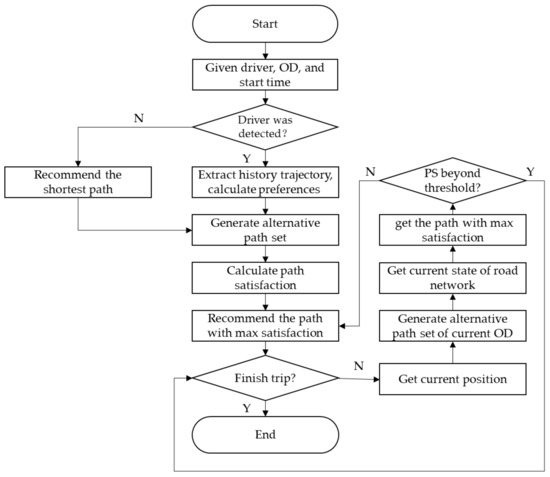
Figure 5.
Personalized path recommendation process.
We aimed to recommend the path with the highest satisfaction to the specific driver given the driver’s information, the OD, and the departure time. First, we extracted the preferences of the driver and the weights of path satisfaction indicators for the driver; otherwise, the driver was assigned preference for the shortest path. Next, a set of candidate paths was generated and the satisfaction S of each path in the set was calculated. Finally, the path with the highest satisfaction was recommended to the driver. At regular intervals, or when passing through an intersection, it was checked whether the current trip was completed. If not, the driver’s current location was obtained and the OD and candidate path set were updated. The road network status was also updated and the satisfaction was re-calculated. If the change in satisfaction exceeded a threshold, paths with higher satisfaction were recommended to the driver. This process continued at each step in time, until the driver completed their current trip.
4.1. Alternative Path Sets
The construction of the candidate path set should take into account the driver’s driving habits and economic considerations, in order to explore better path options. Therefore, the candidate path set was formed by selecting paths with higher frequencies of travel within the OD pair over a period of 7 days, shortest paths between the OD pair, and randomly generated paths. This approach ensured that a variety of potential paths were considered, including those commonly used by the driver, the most efficient ones, and some random alternatives.
4.2. Secondary Path Recommendation Threshold
During a driver’s journey, unforeseen changes in the road network and shifts in driver preferences can occur, leading to potential changes in driver satisfaction to the remaining paths. Therefore, it becomes necessary to provide secondary recommendations for unfinished paths between OD pair while the driver is en route. However, it is important to note that the driver’s perceived path satisfaction may not be highly accurate or continuous, meaning that minor changes in satisfaction may not be sufficient to prompt a decision to change the established path.
Psychology-related studies have shown that an individual’s response to stimulus changes is not solely determined by the magnitude of the change itself, but also by the intensity of the stimulus; that is, the amount of change will only trigger a response from the individual when it reaches a certain ratio in relation to the initial stimulus. In the context of path recommendations, this suggests that a significant change in satisfaction should be required before suggesting an alternative path to the driver.
Therefore, the personalized path recommendation method takes into account this psychological aspect and ensures that a substantial change in satisfaction (i.e., beyond a certain threshold) is required before offering secondary recommendations. This approach balances the need for responding to significant changes in driver satisfaction while avoiding unnecessary path changes triggered by minor variations.
where is the amount of stimulus change, is the current stimulus size, and is the Weber ratio constant. Studies related to the path choice behavior of travelers [29] have shown that the size of this Weber constant is distributed from 5 to 20%. In particular, 10% was chosen as the threshold in this paper, such that only when the change rate of path satisfaction exceeded 10% was a new path recommended to the driver; namely, the threshold of path change was
5. Case Studies
5.1. Research Data
The research area selected for this study was obtained from the road network within Xuancheng City, China, which is characterized by a relatively simple road network structure and comprehensive urban road traffic detection equipment. This enabled the collection of extensive urban traffic information, making it easier to access individual driver information and path data for analysis. The research area encompassed 143 road sections, 91 intersection junctions, and 65 effective electronic bayonets.
To specify the starting and ending points for the study, Figure 6 shows the origin O, located on the northwest side of the road network, and the destination D, located on the southeast side of the road network. This OD pair was situated on opposite sides of the central city of Xuancheng and potential paths passed through the central city area, thus covering a relatively complex road traffic environment. This complexity allowed for observation of travel behaviors among various commuters and was considered representative of the overall transportation patterns. Hence, this OD pair was selected as the target for this study.
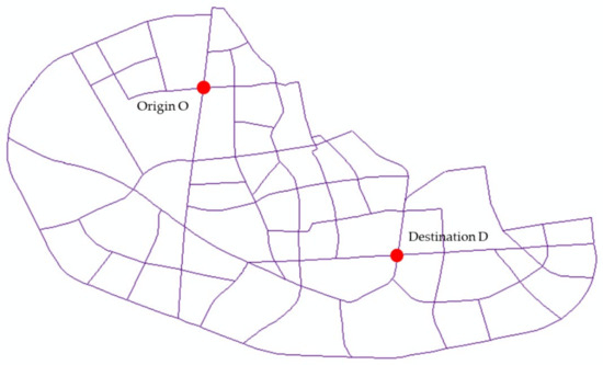
Figure 6.
Target OD pair.
During the specified time period from 12 August 2019 (Monday) to 18 August 2019 (Sunday), a total of 4473 vehicle travel tracks were extracted for the target OD pair in Xuancheng City. It is important to note that the ALPR data only provide information about the intersections passed by the vehicles during their travel, while not directly capturing longer stops or pauses during the journey. Additionally, there may be errors in license plate identification and inaccurate detection timestamps, which can lead to abnormal travel time data.
To ensure the reliability of the travel trajectories, we utilized the average path travel time to exclude obviously incorrect data. Specifically, travel trajectories with an average path speed of less than 5 km/h (common walking speed) or greater than 120 km/h (common maximum speed limit) were considered unreliable. After applying these filters, a total of 4428 valid travel trajectories remained.
Among these valid travel trajectories between the target OD pair, a subset of 644 distinct paths was identified. The distribution of travel trajectories was uneven, with a majority of trajectories concentrated on a smaller proportion of paths. Table 4 presents the seven paths with the highest number of travel trajectories. Among the paths, 33 paths had more than 20 travel trajectories, indicating a relatively higher frequency of usage.
Table 4.
Main travel paths.
The paths in Table 4 are described in the form of node sequences, where the corresponding nodes in the road network are shown in Figure 7; notably, the node number of the origin O is 5122 and the destination D is 4724.
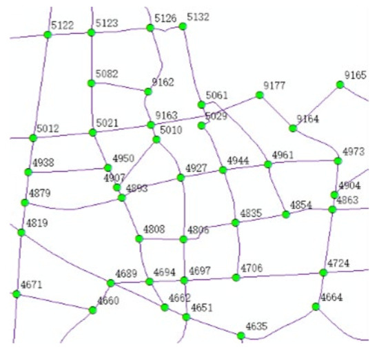
Figure 7.
Nodes and node IDs for OD pairs.
5.2. Calculation of Path Satisfaction of Individual Driver
5.2.1. Path Dynamic and Static Properties
First, the historical travel trajectory data between the target OD were utilized to calculate the dynamic and static attributes of the paths traversed by each trajectory. The dynamic attributes were associated with the departure moment. The static attributes of the three paths depicted in Figure 8 are presented in Table 5. Additionally, the dynamic attributes for the departure time of 12 August 2019 at 8:00 were obtained, which are provided in Table 6.
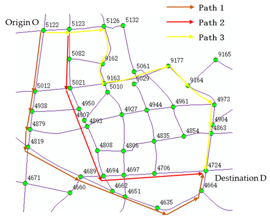
Figure 8.
Path diagram of Path 1, 2 and 3.
Table 5.
Static properties of paths.
Table 6.
Dynamic properties of paths.
Path 1 was the longest, measuring 4811.49 m. It was a straightforward path with fewer intersections and a low turning index. Being a city trunk road, it had multiple lanes and presented relatively high traffic density.
Path 2 had the shortest length, only 4084.65 m. However, it traversed narrow sections with fewer lanes and encountered more intersections. Consequently, it had a higher number of path intersections and a higher path turning index, resulting in increased path density.
Path 3 had a slightly shorter length than Path 1. Its static properties fell between those of paths 1 and 2. With lower traffic density, it was the most frequently chosen path for this OD pair.
These observations highlight the distinct characteristics of the paths between the same OD pair, providing diverse options for travelers with varying preferences.
5.2.2. Path Satisfaction
In this section, we analyze a particular driver’s travel preferences using the method outlined previously. In particular, we calculated the weight of indicators of the driver and determined the driver’s satisfaction with specific paths.
Based on the hierarchical model depicted in Figure 4, we initially computed the value of each indicator in criterion layer B1 through the use of ALPR data. The results are presented in Table 7.
Table 7.
Value for a particular driver’s indicators in criterion layer B1.
Table 7 indicates that the driver’s path selection behavior during the week lacked significant stability, in terms of travel time. While one trip aligned with the historical trajectory, the path difficulty and traffic status for two trips were lower compared to the overall level for all travel trajectories. Thus, it could be inferred that the driver’s preference for path selection was based on the criteria of path difficulty and traffic status.
Utilizing Equation (21), we generated the comparison matrix representing the relationship between the driver’s indicators from layer B1, as detailed in Table 8.
Table 8.
Comparison matrix of criterion layer B1 with respect to target layer A.
The weights of the criterion layer B1 with respect to target layer A were calculated as W_AB1 = (0.104, 0.171, 0.362, 0.362). The consistency ratio was CR = 6.58 × 10⁻¹⁶ < 0.1, indicating that the consistency test was passed.
The percentiles of each indicator in the criterion layer B2, based on all the trajectories, were calculated (see Table 9).
Table 9.
Percentiles for driver indicators in criterion layer B2.
Applying Equation (26) to these data, we calculated the importance scores for each indicator in the criterion layer B2 for the driver, as shown in Table 10.
Table 10.
Value of driver indicators in criterion layer B2.
The comparison matrix and weights for each indicator in criterion layer B2 with respect to criterion layer B1 were calculated, as described below. According to Equation (21), when calculating the comparison matrix of this driver’s criterion layer B2 with respect to criterion layer B11, it is necessary to update the importance scores of indicators applicable to B11 based on the main correlations. As the indicator B11 is mainly determined by B21 path travel time, B22 path length, and B25 number of path intersections, the value of these three indicators were retained and the importance scores of other indicators were set to 0, as shown in Table 11.
Table 11.
Updated value of indicators applied to B11.
The comparison matrix for the criterion layer B2 with respect to indicator B11 was calculated according to Equation (21), as shown in Table 12.
Table 12.
Comparison matrix of criterion layer B2 on indicator B11.
The weights of each indicators in the criterion layer B2 relative to criterion B11 were calculated as follows: . The consistency ratio was < 0.1, indicating that the consistency test was passed.
Additionally, the importance ratings for other criteria within the criterion layer B1 can be found in Table 13, Table 14 and Table 15.
Table 13.
Updated value of indicators applied to B12.
Table 14.
Updated value of indicators applied to B13.
Table 15.
Updated value of indicators applied to B14.
The comparison matrices for the criterion layer B2 relative to other indicators in the criterion layer B1 are presented in Table 16, Table 17 and Table 18.
Table 16.
Comparison matrix of criterion layer B2 with respect to indicator B12.
The weights of each criterion in the criterion layer B2 relative to the criterion B12 were calculated as follows: . The consistency ratio was < 0.1, indicating that the consistency test was passed.
Table 17.
Comparison matrix of criterion layer B2 with respect to indicator B13.
Table 17.
Comparison matrix of criterion layer B2 with respect to indicator B13.
| B13 | B21 | B22 | B23 | B24 | B25 | B26 | B27 | B28 |
|---|---|---|---|---|---|---|---|---|
| B21 | 0 | 0 | −1 | −1 | −1 | 0 | −1 | 0 |
| B22 | 0 | 0 | −1 | −1 | −1 | 0 | −1 | 0 |
| B23 | 1 | 1 | 0 | −1 | −1 | 1 | −1 | 1 |
| B24 | 1 | 1 | 1 | 0 | −1 | 1 | −1 | 1 |
| B25 | 1 | 1 | 1 | 1 | 0 | 1 | −1 | 1 |
| B26 | 0 | 0 | −1 | −1 | −1 | 0 | −1 | 0 |
| B27 | 1 | 1 | 1 | 1 | 1 | 1 | 0 | 1 |
| B28 | 0 | 0 | −1 | −1 | −1 | 0 | −1 | 0 |
The weights of each criterion in the criterion layer B2 relative to the criterion B13 were calculated as follows: . The consistency ratio was < 0.1, indicating that the consistency test was passed.
Table 18.
Comparison matrix of criterion layer B2 with respect to indicator B14.
Table 18.
Comparison matrix of criterion layer B2 with respect to indicator B14.
| B14 | B21 | B22 | B23 | B24 | B25 | B26 | B27 | B28 |
|---|---|---|---|---|---|---|---|---|
| B21 | 0 | 0 | 0 | 0 | 0 | −1 | −1 | 0 |
| B22 | 0 | 0 | 0 | 0 | 0 | −1 | −1 | 0 |
| B23 | 0 | 0 | 0 | 0 | 0 | −1 | −1 | 0 |
| B24 | 0 | 0 | 0 | 0 | 0 | −1 | −1 | 0 |
| B25 | 0 | 0 | 0 | 0 | 0 | −1 | −1 | 0 |
| B26 | 1 | 1 | 1 | 1 | 1 | 0 | −1 | 1 |
| B27 | 1 | 1 | 1 | 1 | 1 | 1 | 0 | 1 |
| B28 | 0 | 0 | 0 | 0 | 0 | −1 | −1 | 0 |
The weights of each criterion in the criterion layer B2 relative to the criterion B14 were calculated as follows: . The consistency ratio was < 0.1, indicating that the consistency test was passed.
The weights of the criterion layer B2 with respect to the target layer A were calculated as
Based on the results depicted in Figure 9, the weights of the criterion layer B2 relative to the target layer A were derived as follows: . It is notable that the maximum of path density had the greatest influence on the driver’s path selection behavior. Table 19 provides the weight table for each indicator within each hierarchy.
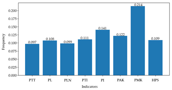
Figure 9.
Satisfaction weights.
Table 19.
Weight values for indicators at each layer.
The driver’s satisfaction with a path was influenced by both the dynamic and static properties of the path. Path 1 in Section 5.2.1 can be taken as an example. Table 20 displays the raw values of the indicators, the percentile values considering all trajectories, and the value of Path 1 at the departure time of 8:00. Using Equation (28), the driver’s satisfaction with Path 1 was calculated as 52.40.
Table 20.
Calculation results for index values related to Path 1.
As outlined in Section 4, the alternative path set was constructed and the satisfaction associated with each path was calculated. In Table 21, the top five paths with the highest satisfaction (along with some path attribute values) are presented.
Among these paths, the three factors that had the greatest impact on the driver were the PMK, PI, and PAK. Notably, the first path in Table 21 exhibited superior attributes, compared to the other paths; namely, it possessed a lower maximum density, a lower number of path intersections, and a low average density, resulting in higher satisfaction when compared to the other paths.
Table 21.
Path satisfaction (partial).
Table 21.
Path satisfaction (partial).
| Paths | PI | PMK | PAK | Satisfaction |
|---|---|---|---|---|
| 5122_5123_5126_5132_5061_4961_4854_4863_4724 | 1.97 | 16.54 | 11.96 | 66.90 |
| 5122_5012_5021_9163_9177_9164_4973_4904_4863_4724 | 1.87 | 23.52 | 13.11 | 54.23 |
| 5122_5123_5126_9162_9163_9177_9164_4973_4904_4863_4724 | 2.14 | 23.52 | 8.95 | 52.40 |
| 5122_5123_5126_5132_5061_4961_4973_4904_4863_4724 | 2.13 | 23.52 | 12.46 | 50.03 |
| 5122_5123_5126_9162_9163_5010_4927_4806_4697_4706_4724 | 2.30 | 30.21 | 15.19 | 41.21 |
5.3. Personalized Path Recommendation Results and Analysis
To validate the feasibility of this method, the aforementioned path recommendation method was utilized to recommend paths to drivers of various types, considering various departure times. A comparison was made with the shortest circuit algorithm, and the results were analyzed.
5.3.1. Differences in Path Selection for Different Types of Travelers
The path selection behavior of a driver during travel is influenced by their various preferences, which are reflected in this study through the weights assigned to the different factors affecting satisfaction. Table 22 presents the satisfaction weights of drivers a, b, c, and d. Driver a primarily considered path difficulty and traffic conditions; driver b relied on personal travel experience and tended to choose familiar paths, placing an emphasis on historical path similarity; driver c prioritized the stability of travel time and preferred paths with minimal risk of delay; and driver d did not exhibit a significant preference, as the influence of each attribute on satisfaction was relatively balanced.
Table 22.
Satisfaction weights for various drivers.
Figure 10 illustrates the path with the highest satisfaction for each driver, considering a departure time of 7:30. The paths are represented by lines of different color. Table 23 provides the actual values and value for the dynamic and static attributes associated with these paths. By analyzing the graphs and data, it is evident that, in the morning peak scenario, the drivers of different types exhibited distinct path selection behaviors. Driver a (who prioritized path difficulty and traffic conditions) selected Path 6 due to its lower average path density, higher maximum path density, and favorable ratings for steering coefficient and number of lanes. Driver b (driven by historical inertia) and driver c (who valued time stability) both chose Path 5, which exhibited attributes that aligned with their preferences. On the other hand, driver d (who had no significant preference) achieved the highest satisfaction with Path 4, as it had the highest importance rating. These results demonstrate that the recommended paths obtained through this method better cater to the individual travel needs of drivers.
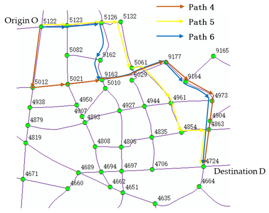
Figure 10.
Path diagram of Path 4, 5 and 6.
Table 23.
Calculation results for index values related to paths 4–6.
5.3.2. Differences in Path Satisfaction at Different Departure Moments
Traffic conditions are subject to time-dependent changes, and the dynamic attributes of a path are closely associated with these conditions. Consequently, the perception of path satisfaction is influenced by these variations, leading to changes in the recommended paths over time. Taking driver a as an example, we recommended different paths at various departure times throughout the day, assessing their respective satisfaction levels. Additionally, we included the satisfaction of the shortest path at different departure times for comparison purposes. The results of the path recommendations are presented in Figure 11.
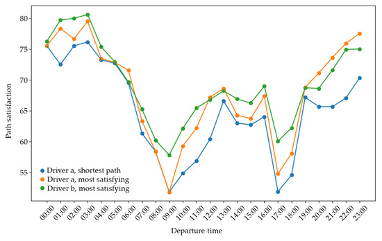
Figure 11.
Satisfaction associated with different paths at different departure times.
The figure illustrates that, for a given path, the fluctuation in path satisfaction primarily arose from changes in its dynamic attributes, including travel time, average path density, and maximum path density, while the static attributes of the shortest path remained unchanged. Table 5, Table 6, Table 7, Table 8, Table 9, Table 10, Table 11, Table 12, Table 13, Table 14, Table 15, Table 16, Table 17, Table 18, Table 19, Table 20, Table 21, Table 22, Table 23 and Table 24 further show how path satisfaction varied throughout the day in response to changes in urban traffic conditions. Two troughs can be observed during the morning and evening peak hours, gradually reaching a local maximum during off-peak hours and ultimately peaking in the early morning hours.
Comparing the satisfaction of paths when considering individual preferences with that when considering only path length, it became evident that satisfaction considering individual preferences consistently surpassed those based solely on length. Furthermore, the extent of the maximum satisfaction relative to the shortest path satisfaction was also influenced by the traffic conditions of the road network. Typically, when the traffic flow density reached its lowest point, the magnitude of the maximum satisfaction over the shortest path satisfaction also reached its peak. This indicated that residents who prioritize good traffic conditions and low path difficulty (such as driver a) may not necessarily have a favorable driving experience during idle and low vehicle density hours when traffic conditions are optimal. In such cases, a more effective approach would be to schedule trips during less congested hours, in order to avoid high traffic density periods. However, it should be noted that these findings were specific to drivers like driver a. Other driver types, such as driver b (see Figure 6, Figure 7, Figure 8, Figure 9 and Figure 10), could still achieve higher levels of satisfaction during peak hours through personalized path recommendations.
These findings highlight the importance of considering the travel preferences of both the drivers (aiming to enhance their travel satisfaction) and traffic managers (seeking to alleviate congestion and guide path selection). Tailoring solutions to address specific preferences is crucial in achieving the desired outcomes.
Table 24.
Comparison of path satisfaction and dynamic attributes.
Table 24.
Comparison of path satisfaction and dynamic attributes.
| Maximum Satisfaction Path | Shortest Length Path | Satisfaction Difference | |||||||
|---|---|---|---|---|---|---|---|---|---|
| Maximum Density | Average Density | Trip Time | Satisfaction | Maximum Density | Average Density | Trip Time | Satisfaction | ||
| 00:00:00 | 3.22 | 1.18 | 463.76 | 75.53 | 3.22 | 1.18 | 463.76 | 75.53 | 0.00% |
| 01:00:00 | 2.68 | 0.88 | 592.11 | 78.32 | 3.98 | 1.95 | 661.24 | 72.51 | 8.01% |
| 02:00:00 | 2.09 | 0.77 | 685.92 | 76.67 | 2.67 | 0.97 | 497.25 | 75.52 | 1.52% |
| 03:00:00 | 1.02 | 0.32 | 532.42 | 79.51 | 2.08 | 0.59 | 284.42 | 76.15 | 4.40% |
| 04:00:00 | 1.64 | 0.91 | 871.10 | 73.47 | 2.66 | 1.49 | 641.79 | 73.25 | 0.30% |
| 05:00:00 | 4.24 | 1.29 | 779.26 | 72.85 | 2.52 | 0.93 | 680.83 | 72.70 | 0.20% |
| 06:00:00 | 8.20 | 3.54 | 862.31 | 71.56 | 8.20 | 5.00 | 717.97 | 69.52 | 2.94% |
| 07:00:00 | 18.10 | 8.39 | 945.95 | 63.33 | 16.54 | 10.20 | 718.94 | 61.31 | 3.30% |
| 08:00:00 | 16.54 | 11.96 | 727.32 | 58.35 | 16.54 | 11.96 | 727.32 | 58.35 | 0.00% |
| 09:00:00 | 21.88 | 13.52 | 755.87 | 51.81 | 21.88 | 13.52 | 755.87 | 51.81 | 0.00% |
| 10:00:00 | 18.92 | 10.79 | 959.73 | 59.25 | 17.97 | 13.12 | 775.78 | 54.82 | 8.09% |
| 11:00:00 | 16.50 | 10.51 | 886.97 | 62.17 | 16.50 | 12.59 | 759.90 | 56.85 | 9.35% |
| 12:00:00 | 14.90 | 7.30 | 887.68 | 67.19 | 14.90 | 11.29 | 728.08 | 60.35 | 11.32% |
| 13:00:00 | 13.54 | 6.03 | 904.93 | 68.58 | 11.29 | 7.34 | 769.79 | 66.56 | 3.04% |
| 14:00:00 | 15.26 | 9.09 | 950.11 | 64.27 | 15.17 | 9.68 | 707.26 | 63.00 | 2.01% |
| 15:00:00 | 16.35 | 9.18 | 915.70 | 63.73 | 16.35 | 9.83 | 678.40 | 62.69 | 1.66% |
| 16:00:00 | 11.50 | 8.54 | 887.95 | 67.36 | 12.94 | 9.85 | 701.07 | 64.01 | 5.22% |
| 17:00:00 | 24.05 | 11.32 | 930.94 | 54.77 | 20.27 | 14.66 | 764.04 | 51.86 | 5.61% |
| 18:00:00 | 20.52 | 10.91 | 941.12 | 58.06 | 18.57 | 13.85 | 721.62 | 54.55 | 6.43% |
| 19:00:00 | 11.28 | 6.51 | 944.51 | 68.77 | 11.28 | 7.23 | 740.56 | 67.16 | 2.40% |
| 20:00:00 | 10.04 | 4.05 | 855.85 | 71.12 | 12.12 | 8.10 | 758.24 | 65.68 | 8.29% |
| 21:00:00 | 12.40 | 3.83 | 676.23 | 73.61 | 12.40 | 8.22 | 747.92 | 65.64 | 12.13% |
| 22:00:00 | 4.71 | 1.72 | 685.59 | 75.92 | 7.39 | 4.28 | 900.27 | 67.06 | 13.20% |
| 23:00:00 | 3.33 | 1.53 | 619.11 | 77.54 | 5.21 | 3.07 | 735.00 | 70.31 | 10.28% |
5.4. Results and Analysis of Mid-Trip Secondary Recommendations
Considering that the traffic conditions in a road network might change, it may become necessary to provide drivers with secondary path recommendations while they are already en route. Figure 12 exemplifies this scenario, taking Path 1 as an example, where drivers were offered secondary path recommendations. As node 4819 experienced significant daily traffic flow, the secondary path recommendation focused on its upstream node (node 4879). Prior to reaching node 4879, the new starting point was set at this node, while keeping the end node unchanged. Separate calculations were then performed to assess the path satisfaction from node 4879 to the end of the originally planned path and for the satisfaction with the newly recommended path. Table 25 presents some of the secondary path recommendation results, where “Change in Satisfaction” denotes the variation in the satisfaction compared to the actual path. The path numbers in the table correspond to those indicated in Figure 12.
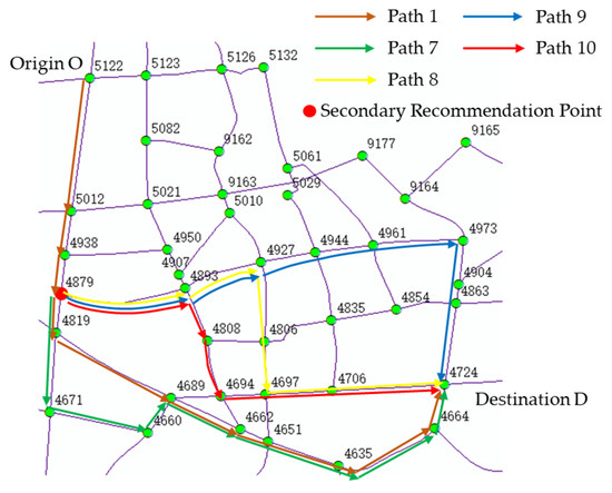
Figure 12.
Path diagram of Path 1, 7, 8, 9 and 10.
Table 25.
Comparison of satisfaction using original vs. secondary recommendations.
The above graphs illustrate selected results for secondary path recommendations from node 5122 and at node 4879 during the time period of 7:00–9:00 on a single day. Based on Equation (30), the chosen threshold for secondary path recommendations in this study was 10%. Therefore, among drivers e, f, and g, only driver e received a secondary path recommendation, resulting in a 42.17% increase in satisfaction. It is worth noting that, for this driver, among the underlying index factors—including path travel time (0.103), path length (0.133), number of path lanes (0.148), path turning coefficient (0.127), number of path intersections (0.128), average path density (0.102), maximum path density (0.115), and historical path similarity (0.144)—historical path similarity carried the highest weight and exerted the most significant influence on the driver. The new suggested path was entirely different from the original path, with a similarity value of 0. Normally, a completely different path should not be recommended. However, through numerical calculations and analysis, it was found that the new path (Path 5) exhibited a significant decrease in maximum path density when compared to the original planned path (Path 7), as well as a lower number of intersections, resulting in a substantial increase in satisfaction. This result demonstrates the necessity and feasibility of quantitative analysis of these indicators.
The above figure showcases only part of the recommendation results. Using a secondary path recommendation threshold of 10%, secondary path recommendations were provided for all 33 drivers who traveled through Path 1 during the aforementioned time period. Among them, 12 drivers experienced a satisfaction increase of more than 10%, indicating that 36.36% of drivers would benefit from a secondary recommendation, demonstrating room for further improvement in individual satisfaction. Prior to the secondary recommendation, the average path satisfaction for all 33 drivers was 45.37. After the recommendation, the average satisfaction increased to 51.16, representing a 12.76% increase. Notably, this exceeded the set threshold for individual perception. Additionally, among the twelve drivers who received the secondary recommendation, five of them (41.67%) were guided from denser main roads to less dense secondary roads, which contributed to traffic flow distribution and helped to alleviate the pressure on main roads.
6. Conclusions
In this paper, we proposed a path satisfaction model based on ALPR data and applied it to a path recommendation method based on individual preferences. The main conclusions of this work are as follows:
- 1.
- Proposed path satisfaction model based on ALPR data
ALPR data were used to extract individual preferences instead of questionnaire surveys, and the pth percentile was used to value indicators in the improved AHP, instead of expert scores. The constructed path satisfaction model could successfully identify the changes in road network status and driver preferences under the scenario designed, providing the basis for personalized path recommendation.
- 2.
- Personalized path recommendation case study
Based on real trajectory data, we extracted the preferences of drivers. Different scenarios were designed to verify the reliability of the satisfaction model, and the satisfaction model was used to conduct a preliminary analysis of the urban traffic conditions. The results demonstrated that the average satisfaction of all drivers was increased by 12.76%, 33.36% of drivers reached the threshold for a secondary recommendation, and 41.67% of the drivers who were given a secondary recommendation were advised to drive from arterial roads to minor roads, thus increasing their satisfaction while reducing the traffic pressure on the arterial roads.
In the future, work should be carried out to address the following areas:
- 1.
- While this study considered changes in traffic conditions due to time variations in making secondary path recommendations, it is worth exploring changes in traffic conditions due to path selections chosen by drivers with multi-agent and reinforcement learning methods.
- 2.
- The individual preferences extracted in this study were based on a fixed OD pair. It is important that whether these preferences can be directly used to all OD pairs, as well as to what extent adjustments are needed to make them applicable to other OD pairs. Further research could determine the conditions under which these preferences can be applied.
Author Contributions
Conceptualization, Y.L. and M.H.; methodology, Y.L. and M.H.; software, Y.L.; validation, Y.L. and M.H.; formal analysis, Y.L. and M.H.; investigation, Y.L. and M.H.; re-sources, M.H.; data curation, Y.L.; writing—original draft preparation, Y.L.; writing—review and editing, Y.L. and M.H.; visualization, Y.L.; supervision, M.H.; project administration, Y.L. All authors have read and agreed to the published version of the manuscript.
Funding
This research was funded by the National Key Research and Development Program of China, grant number 2020YFB1600400.
Institutional Review Board Statement
Not applicable.
Informed Consent Statement
Not applicable.
Data Availability Statement
Not applicable.
Acknowledgments
The authors would like to thank the National Key Research and Development Program of China (2020YFB1600400) for its support. The authors also wish to thank anonymous referees for their valuable comments.
Conflicts of Interest
The authors declare no conflict of interest.
References
- National Bureau of Statistics of the People’s Republic of China. China Statistical Yearbook; China Statistics Press: Beijing, China, 2021.
- Guangzhou Municipal Planning and Natural Resources Bureau (Guangzhou Municipal Oceanic Bureau) Home Page. Available online: http://ghzyj.gz.gov.cn/attachment/7/7104/7104800/7756059.pdf (accessed on 24 April 2023).
- The People’s Government of Guangzhou Municipality Home Page. Available online: https://www.gz.gov.cn/attachment/7/7143/7143318/8495357.pdf (accessed on 24 April 2023).
- Huang, L.; Huang, H.; Wang, Y. Resilience Analysis of Traffic Network under Emergencies: A Case Study of Bus Transit Network. Appl. Sci. 2023, 13, 8835. [Google Scholar] [CrossRef]
- Alawad, H.; An, M.; Kaewunruen, S. Utilizing an Adaptive Neuro-Fuzzy Inference System (ANFIS) for Overcrowding Level Risk Assessment in Railway Stations. Appl. Sci. 2020, 10, 5156. [Google Scholar] [CrossRef]
- Ge, Z.; Du, M.; Zhou, J.; Jiang, X.; Shan, X.; Zhao, X. An Assessment Scheme for Road Network Capacity under Demand Uncertainty. Appl. Sci. 2023, 13, 7485. [Google Scholar] [CrossRef]
- Wang, H.; Zhu, J.; Gu, B. Model-Based Deep Reinforcement Learning with Traffic Inference for Traffic Signal Control. Appl. Sci. 2023, 13, 4010. [Google Scholar] [CrossRef]
- Cao, X.H.; Li, X.Y.; Wei, X.G.; Li, S.; Huang, M.X.; Li, D.L. Dynamic Programming of Emergency Evacuation Path Based on Dijkstra-ACO Hybrid Algorithm. J. Electron. Inf. Technol. 2020, 42, 1502–1509. [Google Scholar]
- Li, Z.J.; Zheng, X.Q.; Wang, S.Q.; Yang, X. Application of Improved A* Algorithm for Path Searching in GIS. J. Syst. Simul. 2009, 21, 3116–3119. [Google Scholar]
- Chang, M.M.; Yuan, L.; Ding, Z.M.; Li, L.T. Adaptive Dynamic Path Planning Method Under Traffic Condition Awareness. J. Transp. Syst. Eng. Inf. Technol. 2021, 21, 156–162+247. [Google Scholar]
- Wang, W.W.; Zhao, X.M.; Li, X.G.; Xie, D.F. Empirical Study and Modeling of Variable Message Signs on Route Choice Behavior. J. Transp. Syst. Eng. Inf. Technol. 2013, 3, 60–64. [Google Scholar]
- Chen, P.Z.; Wu, J.H.; Li, N. A Personalized Navigation Path Recommendation Strategy Based on Differential Perceptron Tracking User’s Driving Preference. Comput. Intell. Neurosci. 2023, 2023, 8978398. [Google Scholar] [CrossRef]
- Liu, X.M.; Lu, X.Y.; Sun, Q.X. Traveler’S Behavior of Path Selection Based on Different Preferences. J. Chongqing Jiaotong Univ. (Nat. Sci.) 2017, 36, 102–106. [Google Scholar]
- Simon, H.A. A Behavioral Model of Rational Choice. Q. J. Econ. 1955, 69, 99–118. [Google Scholar] [CrossRef]
- Zhang, W.H.; Yan, P.; Huang, Z.P. Traveler’s Subjective Path Selection Model Considering Road Network Congestion Status. J. Chongqing Jiaotong Univ. (Nat. Sci.) 2019, 38, 90–95. [Google Scholar]
- Ghader, S.; Darzi, A.; Zhang, L. Modeling effects of travel time reliability on mode choice using cumulative prospect theory. Transp. Res. Part C. 2019, 108, 245–254. [Google Scholar] [CrossRef]
- Li, D.W.; Feng, S.Q.; Cao, Q.; Song, Y.C.; Lai, X.J.; Ren, G. Modeling Route Choice Behavior in the Era of Big Data. China J. Highw. Transp. 2021, 34, 161–174. [Google Scholar]
- Humagain, P.; Singleton, P.A. Investigating Travel Time Satisfaction and Actual Versus Ideal Commute Times: A Path Analysis Approach. J. Transp. Health 2020, 16, 100829. [Google Scholar] [CrossRef]
- Liu, K.; Zhou, J.; Bi, X.X.; Zhang, J.T. Impacts of Traffic Information Type Preference on Urban Travelers′ Route Choice. J. Transp. Inf. Saf. 2019, 37, 71–77. [Google Scholar]
- Correa, D.; Ozbay, K. Urban Path Travel Time Estimation Using GPS Trajectories from High-Sampling-Rate Ridesourcing Services. J. Intell. Transp. Syst. 2022, 2022, 1–16. [Google Scholar] [CrossRef]
- Wang, R.; Zhou, M.; Gao, K.; Alabdulwahab, A.; Rawa, M.J. Personalized Route Planning System Based on Driver Preference. Sensors 2022, 22, 11. [Google Scholar] [CrossRef]
- Dai, J.; Yang, B.; Guo, C.J.; Ding, Z.M. Personalized route recommendation using big trajectory data. In Proceedings of the IEEE 31st International Conference on Data Engineering, Seoul, Republic of Korea, 13–17 April 2015; pp. 543–554. [Google Scholar] [CrossRef]
- Yuan, P.C.; Juan, Z.C. Urban road network evolution mechanism based on the ‘direction preferred connection’ and ‘degree constraint’. Phys. A Stat. Mech. Appl. 2013, 20, 5186–5193. [Google Scholar] [CrossRef]
- Tseng, Y.Y.; Knockaert, J.; Verhoef, E.T. A revealed-preference study of behavioural impacts of real-time traffic information. Transp. Res. Part C 2013, 30, 196–209. [Google Scholar] [CrossRef]
- Long, X.Q.; Su, Y.J.; Yu, C.; Wu, D.X. Analyzing Methods of Vehicle’ Travel Using Plate Recognition Data. J. Transp. Syst. Eng. Inf. Technol. 2019, 19, 66–72. [Google Scholar]
- Saaty, T.L. How to Make a Decision: The Analytic Hierarchy Process. Eur. J. Oper. Res. 1990, 48, 9–26. [Google Scholar] [CrossRef]
- Mirzahossein, H.; Sedghi, M.; Habibi, H.M.; Jalali, F. Site selection methodology for emergency centers in Silk Road based on compatibility with Asian Highway network using the AHP and ArcGIS (case study: I. R. Iran). Innov. Infrastruct. Solut. 2020, 5, 113. [Google Scholar] [CrossRef]
- Li, Y.J.; Zhao, Z.Q. A Judgment Vector in Analytic Hierarchy Process. Syst. Eng. 2002, 2022, 83–87. [Google Scholar]
- Jang, S.; Rasouli, S.; Timmermans, H. Tolerance and Indifference Bands in Regret-Rejoice Choice Models: Extension to Market Segmentation in the Context of Mode Choice Behavior. Transp. Res. Rec. 2018, 2672, 23–34. [Google Scholar] [CrossRef]
Disclaimer/Publisher’s Note: The statements, opinions and data contained in all publications are solely those of the individual author(s) and contributor(s) and not of MDPI and/or the editor(s). MDPI and/or the editor(s) disclaim responsibility for any injury to people or property resulting from any ideas, methods, instructions or products referred to in the content. |
© 2023 by the authors. Licensee MDPI, Basel, Switzerland. This article is an open access article distributed under the terms and conditions of the Creative Commons Attribution (CC BY) license (https://creativecommons.org/licenses/by/4.0/).