Article

A Depression Recognition Method Based on the Alteration of Video Temporal Angle Features

1
College of Computer Science and Technology, Zhejiang University of Technology, Hangzhou 310023, China
2
Computer Intelligent System Laboratory, Zhejiang University of Technology, Hangzhou 310023, China
3
School of Information Science and Engineering, Hangzhou Normal University, Hangzhou 311121, China
*
Author to whom correspondence should be addressed.
Appl. Sci. 2023, 13(16), 9230; https://doi.org/10.3390/app13169230
Submission received: 17 July 2023 / Revised: 9 August 2023 / Accepted: 11 August 2023 / Published: 14 August 2023
(This article belongs to the Section Computing and Artificial Intelligence)

Abstract

:
In recent years, significant progress has been made in the auxiliary diagnosis system for depression. However, most of the research has focused on combining features from multiple modes to enhance classification accuracy. This approach results in increased space-time overhead and feature synchronization problems. To address this issue, this paper presents a single-modal framework for detecting depression based on changes in facial expressions. Firstly, we propose a robust method for extracting angle features from facial landmarks. Theoretical evidence is provided to demonstrate the translation and rotation invariance of these features. Additionally, we introduce a flip correction method to mitigate angle deviations caused by head flips. The proposed method not only preserves the spatial topological relationship of facial landmarks, but also maintains the temporal correlation between frames preceding and following the facial landmarks. Finally, the GhostNet network is employed for depression detection, and the effectiveness of various modal data is compared. In the depression binary classification task using the DAIC-WOZ dataset, our proposed framework significantly improves the classification performance, achieving an F1 value of 0.80 for depression detection. Experimental results demonstrate that our method outperforms other existing depression detection models based on a single modality.

1. Introduction

Depression is a mental disorder characterized by a persistent low mood, typically accompanied by diminished self-esteem, impaired concentration, excessive guilt or self-deprecation, a sense of hopelessness regarding the future, sleep disturbances, and feelings of fatigue or reduced energy [1]. Furthermore, depression exacerbates the risk of suicide among affected individuals, imposing a substantial burden and exerting significant societal impacts [2]. Moreover, a more concerning issue is the ongoing increase in the prevalence of this disease, attributed to various factors, including societal pressures [3].
At present, the diagnosis of depression primarily relies on clinical interviews conducted by doctors and utilizes standardized rating scales, such as the Hamilton Depression Rating Scale (HDRS) [4]. Additionally, self-assessment tools like the Self-Rating Depression Scale (SDS) [5], the Patient Health Questionnaire (PHQ) [6], and the Baker Depression Inventory (BDI) [7] are commonly employed. However, these methods can be influenced by external factors, including the clinician’s expertise and the patient’s tendency to conceal symptoms. Consequently, an accurate automatic diagnosis system [8,9,10] can offer patients effective daily prevention and auxiliary assessment, enabling the early detection of depression and reducing medical costs and societal impact [11].
After the Audio–Visual Emotion Challenge and Workshop (AVEC) [12], numerous scholars have embarked on studying the utilization of text, audio, and visual modalities for depression prediction. According to related studies, facial expressions, vocal features, and semantic features play distinct roles in conveying emotional information [13,14,15]. Facial expressions have shown high reliability and consistency, accounting for 55% of the emotional information. Voice characteristics convey 38% of emotional information, but they are susceptible to interference from distractions such as noise, accents, and background music. In comparison, semantic features, which are emotional expressions based on text analysis, convey only 7% of the emotional information. Due to the influence of language habits, spoken language, abbreviations, and other factors, the processing of semantic features is relatively complex. Considering these factors, in the context of depression recognition algorithms, feature extraction and classification recognition based on video modality data prove to be highly effective. This approach holds the potential for further promotion and application in medical equipment.
In this paper, we present a framework based on visual temporal modality for depression detection. We extract features from patients’ faces in spatial and temporal dimensions using facial landmarks. To address the issue of recognition capability in single-modal depression detection models, we design a feature extraction method that exhibits a strong robustness and low dimensionality. Finally, we utilize the DAIC-WOZ [12] dataset to construct and validate the efficacy of our proposed approach.
The main contributions of this paper are as follows:
(1)
This paper introduces a novel feature extraction method based on facial angle. The method produces facial features that possess translation invariance and rotation invariance. Additionally, it counteracts the interference caused by patients’ head and limb movements through flipping correction, resulting in highly robust extracted features.
(2)
A new model is developed by combining GhostNet with multi-layer perceptron (MLP) modules and video process headers. The model is fine-tuned with respect to the features extracted using the proposed method in this paper. This novel model offers a valuable addition to the depression classification task.
(3)
Extensive experiments are conducted on the DAIC-WOZ dataset to validate the feasibility of the proposed method. The results obtained outperform those of similar methods, establishing the efficacy of the proposed approach.

2. Related Works

Facial expressions and facial movements have a significant impact on nonverbal communication [16,17,18,19]. They reflect an individual’s mental and emotional state and are less influenced by personal subjectivity. Conversely, individuals with depression exhibit distinct facial expressions and movements, typically characterized by frowning, drooping eyes, downturned corners of the mouth, and diminished smiles [20,21]. Analytical modelling based on facial expressions and movements proves to be highly effective in the field of depression recognition.
In the study of facial features, many scholars utilize the Facial Action Coding System (FACS) as the foundation for constructing features. Cohn et al. [22] employed the Active Appearance Model (AAM) to establish 68 facial landmark points, which were subsequently utilized in the classification process. Features such as distance, angle, and area between these landmark points were extracted for analysis. Mclntyre et al. [23] defined facial activity units (AUs) as distinct regions and examined the facial expressions of patients with depression using both original AUs and the defined AU regions. They obtained facial activity patterns based on these analyses. Hamm et al. [24] developed an automated FACS system that calculated the frequency of individual AUs and combined AUs in videos. This system was applied to analyze facial expressions in depressed patients.
Yang et al. [25] utilized a hidden Markov information fusion method to extract the cross-correlation of AU features in a time information sequence, demonstrating its advantages and effectiveness in detecting emotional disorders. Gupta et al. [26] chose structural features, including head movement, eyes opening and closing, the average distance between the upper and lower eyelids, and the distance from the mouth to specific landmarks. Nasir et al. [27] examined facial landmarks as a time series, investigating displacement, velocity, and acceleration as motion-related features, and attained the highest performance indicators in the AVEC2016 competition.
Pampouchidou et al. [17] encoded facial landmark features into grayscale images, generating the Landmark Motion History Image (LMHI) of facial landmarks. White pixels represent the most recent motion, while the darkest grey represents the earliest motion. Grayscale image extraction was performed using Local Binary Patterns (LBPs) and Histogram of Oriented Gradients (HOGs) features. Wang et al. [28] proposed Sampling Sliced Long Short-Term Memory Multiple Instance Learning (SS-LSTM-MIL), a multi-instance learning method that utilizes two-dimensional facial key points as input. This approach employs LSTM and pooling techniques for detecting facial depression in specific video segments. Sun et al. [29] presented the Robust Adversarial Adaptation (SRADDA) method, which addresses domain adaptation across varying scales, label spaces, and depression severity assessments in deep evaluation networks.
The previous studies demonstrate that these facial features rely on a human clinical understanding of depression. These features are derived by quantifying geometric properties like distance, angle, and area to analyze the facial changes exhibited by individuals with depression. Dynamic information regarding features is represented through the calculation of speed and acceleration for each motion frame. Nevertheless, this method of feature extraction leads to the loss of both the topological structure information of the face and additional features that go beyond clinical understanding.
This paper presents a framework for depression detection based on visual temporal modality. Facial landmarks are utilized to extract features from patients’ faces in both spatial and temporal dimensions. A feature extraction method is then designed to classify depression, addressing the limitation of single-modal depression detection models. The method exhibits strong robustness and low dimensionality.

3. Proposed Framework

The framework is comprised of three main components: feature extraction and training unit acquisition, GhostNet neural classification network, and aggregation classification. As shown in Figure 1. Each of these components will be introduced in detail in Section 3 and Section 4, respectively.
This article establishes two concepts regarding angles for the ease of subsequent discussions:
Definition 1.
Target angle: In the target plane, the angle between two straight lines is called “angle” for short.
Definition 2.
Target image angle: In the image plane, the angle between two straight lines is called “image angle” for short.

3.1. Facial Landmark Detection

Facial landmark detection is a computer vision technique [30] that automatically detects the locations of specific points (e.g., eyes, nose, mouth) in facial images. These specific points are commonly referred to as facial landmarks or face landmarks.
This paper utilizes the facial landmark detection method proposed by Tadas et al. [29,30]. The method establishes 68 landmark points on the human face, comprising 17 points for face shape, 10 points for eyelashes, 12 points for the nose, and 18 points for the mouth. These 68 landmark points provide a more intuitive outline of the human face model. Figure 2 illustrates the impact of facial landmark detection.

3.2. Angle Selection Method

The fundamental principle of feature selection is to accurately capture the angle of expression change. This paper selects the following angles as the features representing facial expression changes, based on this principle.
The face is analyzed using the key point detection method described in Section 3.1, resulting in the extraction of 68 marker point positions. The 68 landmarks are assigned numbers ranging from 1 to 68. The numbering sequence is provided in Table 1.
In feature A 18 , Le = mean(37~42) represents the centroid position of the left eye, while Re = mean(43~48) represents the centroid position of the right eye. Here, mean(∙) denotes the function for calculating the average value.
Each feature carries a distinct significance and can partially depict the variations in facial expressions. For instance, when individuals smile, their eyes contract into a line, while they widen when experiencing fear. The selected features A 5 to A 8 in this study are capable of reflecting these changes in facial expressions.

3.3. Robustness Analysis of Angle Features

Facial expressions primarily manifest through variations in angle information. For instance, a smile is characterized by an upward movement of the corners of the mouth, while intense crying involves a downward movement of the corners of the mouth. In this paper, we extract features A 11 to A 14 to precisely capture these expression changes. Human head movement can be decomposed into six components: horizontal translation (x-axis), vertical translation (y-axis), depth translation (z-axis), yaw rotation (left/right tilt), pitch rotation (head up/down), and roll rotation (left/right head). It is important to investigate whether these six actions have an impact on our angle features and if the features extracted in this study effectively withstand the influence of these actions, thus demonstrating their robustness. The subsequent section presents an analysis and discussion on the robustness of these features.

3.3.1. Rotation Invariance

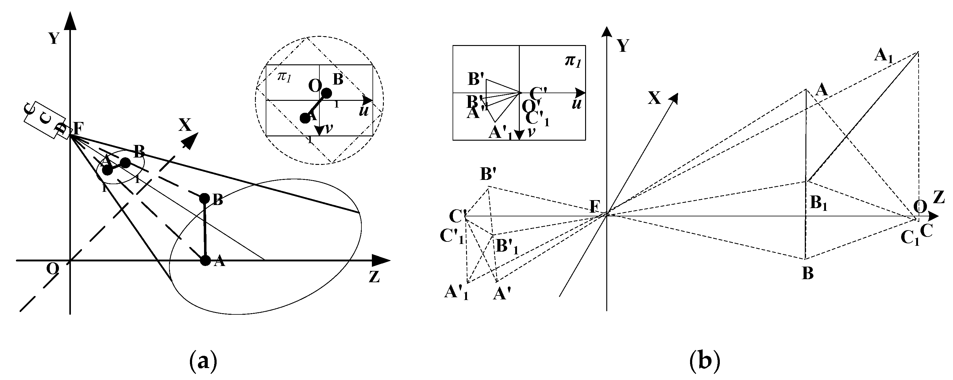
The target undergoes rotation along the z-axis, as depicted in Figure 3. Patients frequently tilt their heads to the left and right during the recording of the interrogation video. Consequently, the tilting of the patient’s head to the left and right can be considered facial rotation.
Theorem 1.
LetABC be an image on the target surface π after camera imaging, and letA′B′C′ be its corresponding image. When the target rotates along the z-axis, the angles ∠A′B′C′, ∠B′A′C′, and ∠B′C′A′ remain unchanged. This property is referred to as the rotation invariance theorem.
Proof of Theorem 1.
The rotation of the target around the z-axis is equivalent to the rotation of the camera around the optical axis. Figure 3a is the imaging model when the camera rotates around the optical axis, and Figure 3b is the imaging model when the target rotates around the z-axis. By establishing the camera space coordinate system O X Y Z , as shown in Figure 3a, let A 1 B 1 be the image of target A B in image plane π 1 . When the camera rotates to shoot, although the image A 1 B 1 of the target A B will change relative to the image coordinates, the length | A 1 B 1 | of A 1 B 1 will not change. This is shown in the vignette in Figure 3a. Thus, the following conclusions can be drawn: in the process of target rotation, the length of the image obtained by obliquely shooting the target at any angle will not change.
Let the image of target A B C be A B C ; when the target point A B C rotates around the z-axis, a new target A 1 B 1 C 1 is formed, and correspondingly, there is a new corresponding image A 1 B 1 C 1 on the image plane. According to the theory of target rotation around the z-axis, there is the following Formula (1):
A 1 B 1 = A 1 B 1 A 1 C 1 = A 1 C 1 C 1 B 1 = C 1 B 1
That means A B C A 1 B 1 C 1 . Therefore, the image angles A B C , B A C , B C A will not change with the change of the target rotation. □

3.3.2. Translation Invariance

Translation involves the parallel displacement of a target point along the X, Y, or Z-axes within the OXYZ plane. In the context of a patient’s medical examination, it refers to bodily movements such as flexion, extension, lateral shifting, as well as anterior and posterior shifting.
Theorem 2.
Let the image of any  A B C  in the target surface  π  after the camera imaging be  A B C ; when the target  A B C  translates arbitrarily along the x-axis, y-axis, or z-axis, the image angles  A B C , B A C , B C A  do not follow the target changes in position. Hence, this property is referred to as the translation invariance theory.
Proof of Theorem 2.
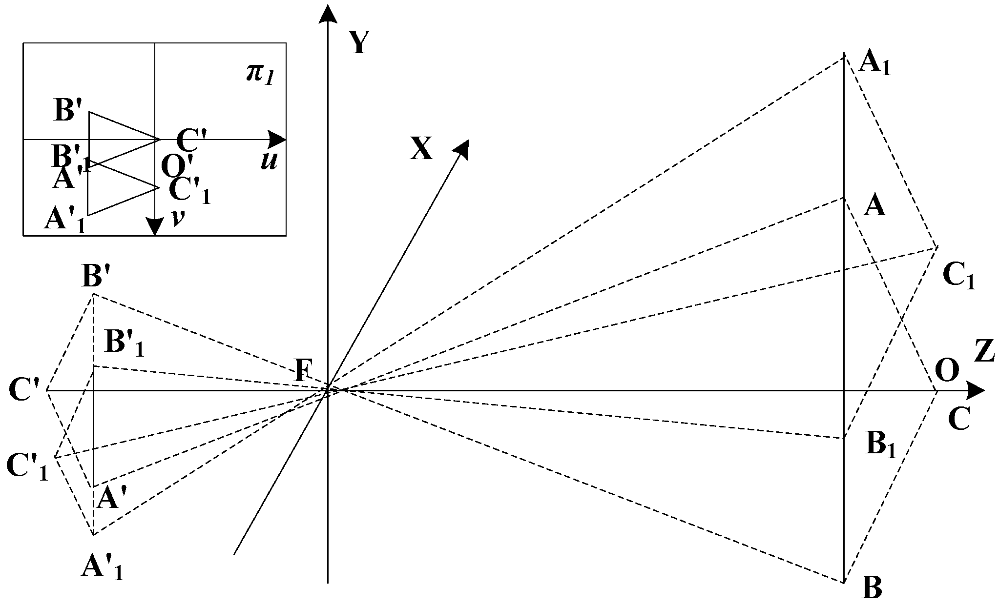
Establish the coordinate system shown in Figure 4, set the image of triangle A B C in image plane  π 1 as A B C , move triangle A B C to A 1 B 1 C 1 along the y-axis, and the image of triangle A 1 B 1 C 1 is A 1 B 1 C 1 .
According to the principle of pinhole imaging, triangle A B C is similar to triangle A B C . The following Formula (2) represents this relationship:
A B C A B C
When triangle A B C moves to A 1 B 1 C 1 along the y-axis, triangle A B C will not be deformed due to parallel movement, so there is a congruent relationship between triangle A B C and triangle A 1 B 1 C 1 . There is the following Formula (3):
A B C A 1 B 1 C 1
Triangle A 1 B 1 C 1 is the image of triangle A 1 B 1 C 1 , and so, there is the following Formula (4):
A 1 B 1 C 1 A 1 B 1 C 1
Then, it can be concluded that triangle A B C and triangle A 1 B 1 C 1 have a similar relationship. There is the following Formula (5):
A B C A 1 B 1 C 1
Thus, the image angles A B C , B A C , and B C A do not change as the target moves along the y-axis. Similarly, when the target moves along the x-axis and z-axis, the image angle will not change either. □

3.4. Flip Correction

Human head movements commonly involve shaking the head laterally (left and right deflection) as well as tilting it upward and downward (referred to as pitch movement). The lateral deflection (roll) and pitch movement have a significant impact on the angular properties, consequently influencing facial expression recognition. Angle correction is essential to address changes in angular properties caused by target flipping. To achieve accurate flipping correction, it is crucial to comprehend the relationship between the flipping angle, target angle, and image angle in the two given scenarios.

3.4.1. When the Target Is Flipped Horizontally, There Exists a Relationship among the Target Angle, Image Angle, and Flip Angle

The target’s left and right deflection, known as “Roll”, indicates rotation around the y-axis or a parallel straight line. Deflection of the target surface in the left and right directions causes a change in the image angle.
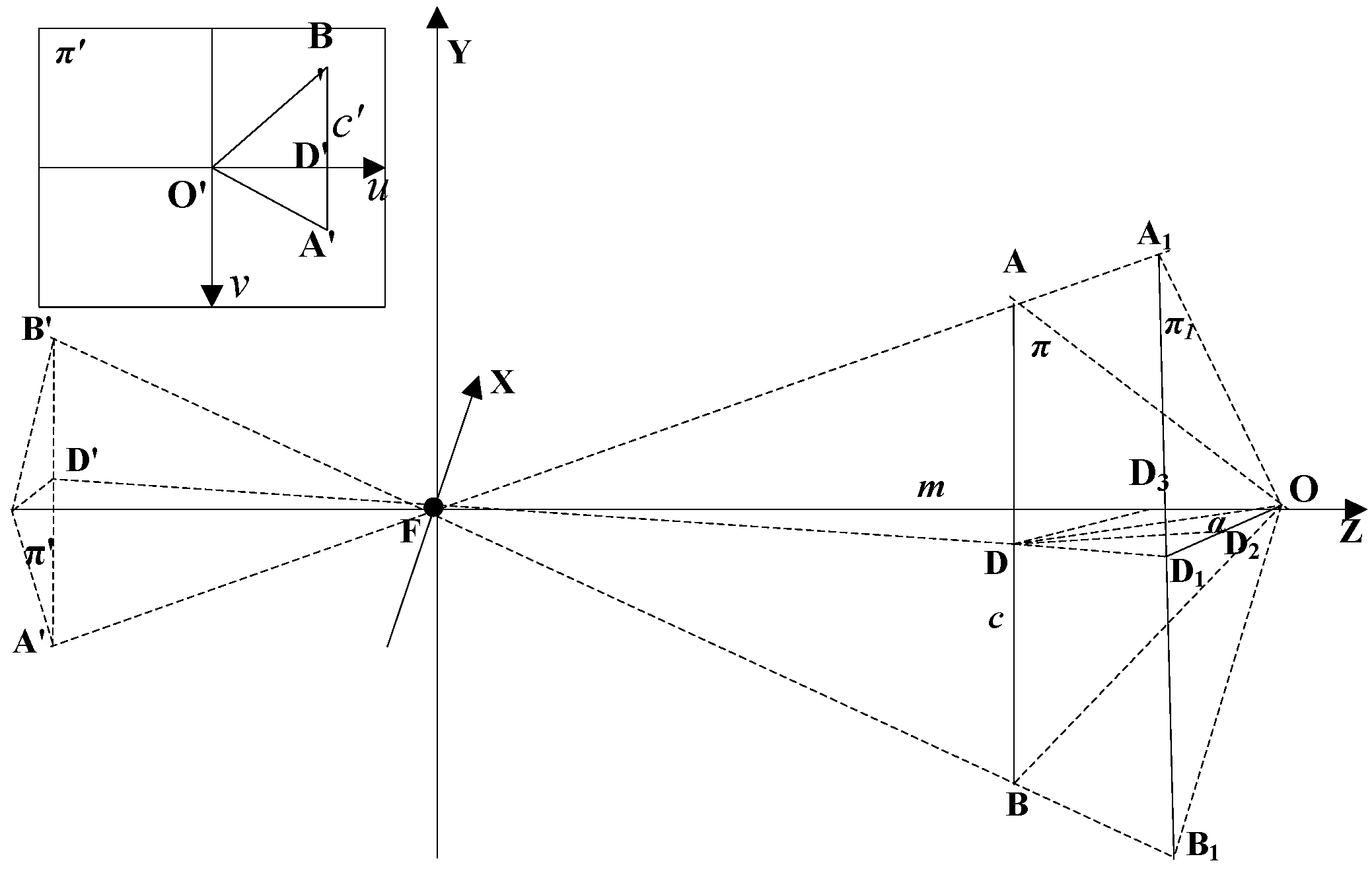
First, establish a space coordinate system X F Y as shown in Figure 5, where the point F is the optical center of the camera. Assuming that A B is parallel to the y-axis, and the image of A B is A B , in the image plane π , establish the u O v plane coordinate system, where u and v represent the horizontal axis and the vertical axis, respectively. Obviously, the A B and v axes are parallel. Suppose the intersection point of the target and the main optical axis of the camera is O , and a plane π parallel to the image plane π 1 is made through point O , connect F A and extend π to intersect A 1 , connect F B and extend π to intersect B 1 . A B intersects u axis at D , connects D F and extends, and intersects A B , A 1 B 1 at D , D 1 , respectively. Connect O D and O D 1 . In plane X F Z , a straight line parallel to the z-axis passing through point D intersects O D 1 at point D 2 , and a straight line drawn through point D along O D 1 intersects the z-axis at D 3 .
Because π is parallel to π 1 , there is the following Formula (6):
A O B = A 1 O B 1
Let A 1 O B 1 = ϕ , A 1 O D 1 = ϕ 1 , B 1 O D 1 = ϕ 2 , A O B = θ , A O D = θ 1 , B O D = θ 2 . and ϕ 1 + ϕ 2 = ϕ , θ 1 + θ 2 = θ . Set the distance between point O and the optical center of the camera as m , that is, F O = m . Also, set the distance from point O to line segment A B as d , that is, O D = d . Suppose the length of line segment A B is c , the length of A D is c 1 , and the length of B D is c 2 , then there is c 1 + c 2 = c . Let α be the angle between plane O A B and plane π 1 . Since D D 2 O D 1 , then there is the following Formula (7):
D D 2 = d × sin α D D 3 = d × cos α
: D F D 3 D 1 F O , :
O D 1 = m × d × cos α m d × sin α
: D F A D 1 F A 1 , :
A 1 D 1 = c 1 × m m d × sin α
In D 1 O A 1 , there is the following Formula (10):
tan ϕ 1 = A 1 D 1 O D 1 = c 1 d × cos α
: tan θ 1 = c 1 d , :
tan ϕ 1 = tan θ 1 cos α
In the same way, there is the following Formula (12):
tan ϕ 2 = tan θ 2 cos α
To sum up, the relationship between the angle in the target image (referred to as the image angle) A O B , the target angle A O B , and the deflection angle α can be obtained:
ϕ = ϕ 1 + ϕ 2 tan ϕ = tan θ 1 cos α tan ϕ 2 = tan θ 2 cos α θ = θ 1 + θ 2 ,   α π / 2 , π / 2
It can be obtained from Formula (13) that when the target A O B moves around the point O parallel to the y-axis, its image angle ϕ has no relevance with the distance m between the target point O and the optical center of the camera. The relationship between ϕ , θ , and α is shown in Figure 6.
It can be determined from Figure 6 that when the face is not deflected, that is, α = 0 , the target angle θ and image angle ϕ will be equal in value. And when the face is deflected, α 0 . The target angle θ will not be the same as the image angle ϕ , and the image angle ϕ will definitely be greater than the target angle θ . The flip action then disturbs the angular characteristics. To mitigate this interference, the approach involves capturing a frontal shot of the face, extracting relevant values at specific angles that remain unaffected by facial expression changes, and subsequently applying corrections to other face frames using Formula (13). Detailed information on obtaining a front face photo can be found in Section 3.5.1.

3.4.2. When the Target Is Flipped Vertically, There Exists a Relationship among the Target Angle, Image Angle, and Flip Angle

The target flips up and down (pitch), which means that the target rotates around the x-axis or a line parallel to the x-axis. When the target flips up and down, the image angle will change.
Due to the symmetry of camera imaging, there is symmetry between left and right deflections and up and down flips; thus, simply swap the x-axis and y-axis in Figure 5 to obtain the relationship between the target angle, image angle, and flip angle when flipping up and down.
Let the flip angle be β , and, according to the symmetry, the relationship between them can be obtained:
ϕ = ϕ 1 + ϕ 2 tan ϕ 1 = tan θ 1 cos β tan ϕ 2 = tan θ 2 cos β θ = θ 1 + θ 2 ,   β π / 2 , π / 2
In Formula (14), ϕ and θ have the same meaning as Formula (19).

3.4.3. Deflection/Flip Correction Method

From Formulas (13) and (14), it can be seen that if the target angle can be known in advance, then the deflection/flip angle can be solved. In this paper, A 18 is used for flip correction, and either A 19 or A 20 is used for deflection correction.
For angle A 18 ( A n g ( L e , 31 , R e ) ) , point L e is the center point of the left eye, point 31 is the tip of the nose, and point R e is the center point of the right eye. These three points will not move with the change of expression, which means that the angle information formed by these three points does not become larger or smaller with facial expressions, but does increase or decrease in size accordingly with flipping up and down. Therefore, flip correction can be performed by means of this one feature.
Suppose there is a frame of frontal image I , then let A n g I L e , 31 , R e = θ , and then θ is calculated by Formula (15):
θ = A C B = cos 1 B C 2 + A C 2 A B 2 2 B C A C  
Another frame of image I 1 is set, so A n g I 1 L e , 31 , R e = ϕ can be calculated by Formula (15), Similarly, the flip angle β of the image I 1 relative to the reference frame I can be calculated by Formula (14).
When the flip angle β is obtained, the error caused by the flip of some features can be corrected. It is advisable to set the angle to be corrected as A i U D , then A i U D is calculated by Formula (16):
A i U D = tan 1 cos β × tan A i
A i in Formula (16) is the image angle, and the image angle can be obtained by Formula (15).
In the same way, angle A 19 or A 20 can be used to correct the left and right deflection of some angles that need deflection:
A i L R = tan 1 cos α × tan A i

3.5. Feature Extraction and Training Unit

Figure 1 illustrates the initial stage of the framework, which involves feature extraction and training unit acquisition. Feature extraction in the first stage is divided into two steps: (1) the selection of a reference frame and (2) the extraction of angle features using difference calculation. The acquisition of training units, i.e., multiple instances of a video, is accomplished using the active Windows mechanism. Subsequently, the feature extraction process is described.

3.5.1. Determine the Reference Frame

The reference frame image must have the patient’s face plane parallel to the image plane, that is, the frontal photo of the patient’s face. Although it may not be possible to find a frame with the face plane parallel to the image plane during the patient’s consultation process, it is necessary to identify the frame in the diagnosis video that is closest to the parallel image plane. In this scenario, we simply identify the frame image closest to the image plane and use it as the reference frame image.
From formulas (13) and (14), it can be known that when the head does not deflect and flip, that is, α = β = 0 , the face plane and the image plane are parallel, and the image angle ϕ is exactly equal to the target angle θ . When there is a deflect and flip situation, the image angles A 18 , A 19 , and A 20 will decrease as well. Therefore, only one frame of image needs to be found so that Formula (18) holds:
I j = max I j j = 1 , 2 , , n A 18 + A 19 + A 20
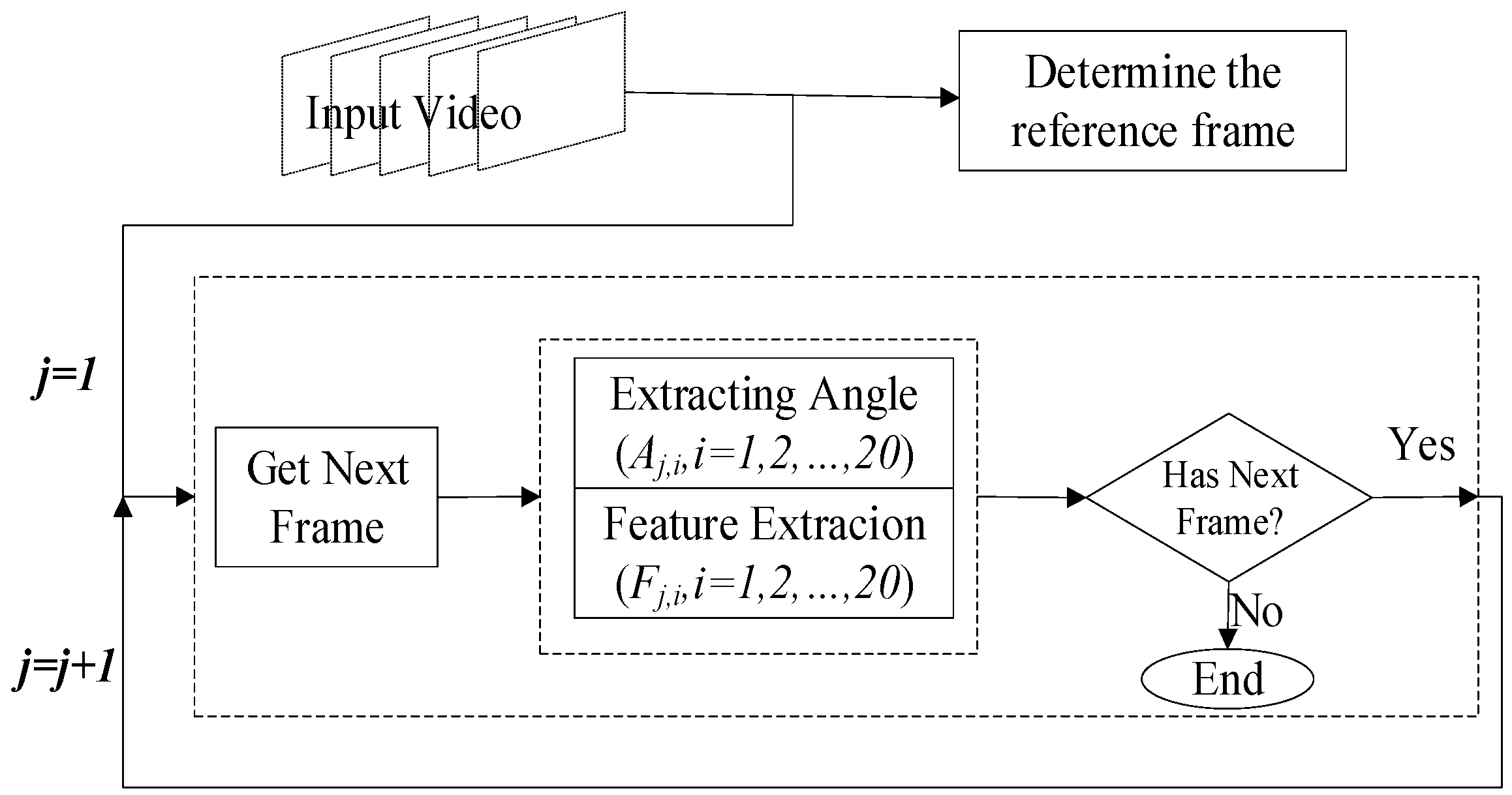
When a reference frame satisfying Formula (18) is found, use Formula (18) to calculate all A 1 ~ A 20 in Table 1, denote it as A r e f , 1 ~ A r e f , 20 , and save it. Among them, the three angles of A 18 , A 19 , and A 20 will be used as hyperparameters in the flip correction of the feature extraction process (Figure 7); n is the number of video frames.

3.5.2. Difference Extraction of Angle Features

In order to accurately describe changes in expression and mitigate misjudgment caused by deflection and flip actions, the angle feature extraction scheme aims to minimize their influence. To achieve this objective, Figure 7 illustrates the designed process for angle feature extraction in this paper.
In Figure 7, the “Determine the reference frame” step yields certain correction parameters, which are subsequently utilized for flip correction in the feature extraction process, as depicted in step 1 below. And in Figure 7, The “feature extraction” step must execute the following specific operations:
(1)
Flip correction: Use Formulas (16) and (17) to correct the deflection and flip of the angle of this frame, and obtain A i = 0.5 × A i U D + A i L R , i = 1 , 2 , , 20 .
(2)
Feature calculation: Calculate the expression difference between the two frames before and after; then, the feature F j , i is calculated by:
F j , i = A j , i A j 1 , i ,   i = 1 , 2 , , 20 ,   j = 1 , 2 , , n 1
n in Formula (19) is the total number of frames that can detect expressions.
Following the above feature extraction process, we obtain the original input data needed for the experiment from the video. The subsequent step involves partitioning the original feature data into training units.

3.5.3. Training Unit Acquisition

A training unit refers to the extraction of several instances from a single piece of datum, where each instance serves as a representative of that particular datum. For instance, in the case of experimental data obtained from a subject without mental illness, the majority of instances are likely to be non-mental illness in nature. In this paper, a sliding window is employed for reference, enabling the extraction of multiple instances on a larger scale. This technique transforms one sample into multiple instances of the same scale. Regarding the size of the sliding window, we specify the parameters in Section 4.3. of the experimental dataset introduction.

4. Experimental Studies

4.1. GhostNet

GhostNet [31] is a lightweight neural network with several key features. Firstly, it demonstrates a high efficiency when compared to other neural network structures like ResNet [32] and MobileNetV2 [33]. GhostNet achieves this through faster processing, fewer parameters, and reduced calculations. Secondly, GhostNet utilizes group convolution technology, dividing the convolution kernel into smaller groups. This approach reduces parameter size and calculation requirements for each convolution layer, resulting in an improved operational efficiency. Thirdly, GhostNet incorporates a channel attention mechanism. This involves adding a channel attention module after each convolutional layer to dynamically adjust the weight of each channel. This adjustment enhances the network’s learning capability. Lastly, GhostNet introduces a feature reorganization mechanism. This involves rearranging the feature maps generated by different convolutional layers to further enhance training efficiency and network accuracy.
The Ghost Module (GM) [31] in Figure 8 consists of three steps, namely conventional convolution, Ghost generation, and feature map splicing.
(a)
First, by providing the input data X R c × h × w , use the convolution operation to obtain the intrinsic feature map Y R h × w × m . Where c is the number of input channels, h and w are the height and width of the input data.
Y = X f
where f R c × k × k × m is the convolution kernel, k × k is the size of the convolution kernel, and the bias term is omitted.
(b)
In order to obtain the required Ghost feature map, each feature map y i of Y is used to generate a Ghost feature map with operation Φ i , j .
y i j = Φ i , j ( y i ) ,     i = 1 , . . . , m , j = 1 , . . . , s ,
(c)
The intrinsic feature map obtained in the first step and the Ghost feature map obtained in the second step are spliced (identity connection) to obtain the output of the Ghost module.
Inspired by the work presented in [31,34,35,36,37], we made changes to GhostNet based on the following factors: (1) In our video classification task, the initial input channels vary from traditional images. For images, the initial channel number is 3, representing the RGB channels. However, in this paper, the initial channel number corresponds to the total number of each feature angle designed in Section 3.1. (2) While largely preserving the original GhostNet structure, this section selectively modifies the second part of GhostNet’s structure, specifically the GhostNet Bottleneck, with the objective of employing GhostNet as a bottleneck graph to extract the network’s backbone. (3) The fourth part of GhostNet, which comprises an FC neural classification network, has been removed and replaced with a 4-class MLP [32] structure for classification purposes. The revised network structure is depicted in Figure 8, and the video processing head is used to shape the unit to fit the GhostNet input.
In addition, we have included Table 2, which presents data to facilitate the understanding of the modifications made in GhostNet. The current GhostNet network consists of approximately 2.7 M parameters, and the flops (floating-point operations) are around 1.0 G. The specific parameters in the network structure depicted in Figure 8 are listed in Table 2.
Table 2 presents the following designations: G-bneck refers to the GhostBottleneck module, #exp represents the expansion distance, #out signifies the number of output channels, and SE indicates the usage of the SE module.

4.2. Aggregate Classification

In the PHQ-8 scale [38], the scoring is as follows: 0–4 points indicate no depression, 5–9 points suggest mild depression, 10–14 points indicate moderate depression, and a score of 15 or higher indicates moderate to severe depression.
The four types of pseudo-labels (1, 2, 3, and 4) correspond to different PHQ-8 scores, denoted as P H Q s . The general depression consultation data will only provide tags corresponding to the entire duration of the long video. To transform the depression classification task of long videos into the score classification task of segmented short time series units, a new label must be created for each unit.
Based on depression-related research findings, the short-sequence units corresponding to pseudo-label 4 have been found to be more significant than those corresponding to pseudo-labels 1, 2, and 3 in assessing depression. However, the frequency of facial changes corresponding to label 4 is lower throughout the entire video. Thus, we developed a score aggregation function for adjusting the weights of various pseudo-labels during the aggregation process.
Assuming that video V has l short time series units, the model output label of the i t h ( 0 < i l ) short time series unit is denoted as v n . All short sequential units can be expressed as V = v 1 , v 2 , v 3 , . . . , v l . Then, the expression of the score aggregation function is as follows:
s ^ V = 1 l i = 1 i = l ρ 1 × v i       ( i f   v i = 1 ) ρ 2 × v i       ( i f   v i = 2 ) ρ 3 × v i       ( i f   v i = 3 ) ρ 4 × v i       ( i f   v i = 4 )
For the weight parameters ρ 1 , ρ 2 , ρ 3 , and ρ 4 , we make selections via the differential evolution algorithm [39]. Finally, we determine whether the corresponding patient suffers from depression by judging whether the aggregated score s ^ is greater than the set threshold.

4.3. Experimental Dataset

The DAIC-WOZ dataset [12] is mainly video, audio, and questionnaire survey data collected to diagnose mental disorders such as depression and anxiety. This dataset is referenced in the Depression Recognition Task Module in the 2014 and 2016 AVEC competitions. The interviews are conducted through situational dialogues between the virtual interviewer, Ellie, and the subjects to elicit corresponding emotional responses and record the characteristics in real-time. According to official standards, the entire dataset exposes 189 sample data and is divided into 107 training sets, 35 validation sets, and 47 test sets. Since no official public label indicates whether the subjects in the test set are depressed or not, this paper employs only 142 sample data from the combined training and test sets to ensure the accuracy and validity of the experimental results. Moreover, to safeguard privacy, the DAIC-WOZ dataset does not provide the original video data but instead offers the 2D coordinate data of facial landmarks extracted by OpenFace [30]. Therefore, the experiment in this paper directly utilizes the provided coordinate data of facial landmarks, eliminating the need for facial landmark extraction steps. The detailed classification of depression or non-depression in the sample data is shown in Table 3.
In this paper, the DAIC-WOZ dataset was utilized, and a sliding window approach was implemented to sample the original data. The window size was set to 120 s, with an overlap size defined as 1/6 of the window size. The original data consisted of video samples at a rate of 30 Hz. During the data cleaning process, a filter was applied to exclude video frames with a face confidence lower than 0.7 from the original video. This filtering process aimed to mitigate the influence of significant face deflection or flipping on the experimental results.

4.4. Experimental

4.4.1. Evaluation

In this paper, the GhostNet network is chosen as the feature extraction network and modified to suit the input. An MLP [36] is employed for four-class classification. The original video data consist of 20 feature angles across 3600 frames, which are reshaped into a 60 × 60 × 20 input format. The learning rate plays a crucial role in optimizing neural networks. For this experiment, the Adam optimizer [40] is utilized. The initial learning rate is set to 0.001 and reduced to 0.1 times the original rate at the 200th and 400th epochs, respectively. S o f t l a b e l is used during training to calculate the loss, mitigating the impact of hard labels on network training. S o f t l a b e l is calculated as follows:
S o f t l a b e l = 1,0 , P H Q s 5 10 P H Q s / 10 , 0 , 6 P H Q s < 9 0 , P H Q s 9 / 10 , 9 P H Q s < 14 0,1 , P H Q s 14
In this paper, precision rate (P), recall rate (R), and F1 value (F-score) are used as the evaluation indicators of sentiment polarity classification. The calculation formula is as follows:
P = T P / T P + F P
R = T P / T P + F N
F 1 = ( 2 × P × R ) / ( P + R )

4.4.2. Experimental Results Comparison

The methods employed in this paper involve extracting one-dimensional or multidimensional modal features from the patient’s face, voice, and text data. These extracted features are then used for training and verification on various neural networks.
Table 4 provides a comprehensive comparison between our developed unimodal depression algorithm based on facial features and previous studies utilizing different modalities. The designed features demonstrate commendable performance in terms of precision rate, recall rate, and F1 score, achieving values of 0.77, 0.83, and 0.80, respectively.
Manoret et al. [41] obtained the result of a mixed model of multiple neural networks, including CNN and LSTM, with a recall rate of 0.91. However, the precision rate of this algorithm is only 0.64, resulting in a final F1 of 0.75, which is 0.05 lower than the one proposed algorithm in this paper. Additionally, the F1 scores of Othmani [14] and Rejaibi et al. [42] in the audio single-mode design algorithm are 0.30 and 0.34 lower, respectively, compared to the performance achieved by the features designed in this paper.
Text is considered unimodal due to its characteristic of containing precise information. The F1 score of the text single-modal feature proposed by Sun et al. [13] is 0.23 lower compared to this paper. Dinkel et al. [39] and other researchers effectively utilize text features by employing the BGRU neural network for processing text information after performing word embedding (Word2Vec) on the text data, resulting in an F1 value that is 0.04 higher compared to ours. Additionally, when comparing with the multimodal detection algorithms proposed by Arioz [44] and Lam et al. [45], it is evident that the algorithm presented in this paper outperforms them in terms of precision, recall, and F1 scores when utilizing mixed modes.
To objectively evaluate the algorithm proposed in this paper, we compare the video modality used in this paper with other algorithms, including video modality. The comparison results are presented in Table 5.
The results presented in Table 5 demonstrate that the features proposed in this study yield remarkable improvements in algorithm performance. Wei et al. [47] achieved a precision rate of 0.89 in their three-modal (visual + audio + text) fusion, surpassing the pure visual mode in this study by 0.12. However, the recall rate was adversely affected, leading to an F1 value 0.1 lower compared to this paper. Haque et al. [49], utilizing the Causal Convolutional Network (C-CNN), achieved a similar recall rate to this study in multimodal analysis. However, their F1 value was 0.03 lower compared to this paper. Conversely, both Wang [28] and Song [46] utilized visual modality data in their studies. In general, the algorithm proposed in this study excels at extracting features from the pure visual modality, leading to superior outcomes.
In the DAIC-WOZ dataset [12], we are provided with several types in terms of visual modal data, including head Pose, eye annotation direction Gaze, and 2D face68 key points. Table 6 presents our method and the results of Guo et al. [50] using the time–space expanded convolutional network (TDCN) and feature attention module (FWA) in different video modalities. Among all the visual modalities. The effectiveness of our method is second only to the approach that utilizes the mixed visual information of facial key points and head pose simultaneously. The F1 values are only 0.1 lower than those achieved by that approach.
As shown in Table 6, when using Gaze data alone, they obtained an F1 value of 0.63, whereas our method achieved a 0.17 higher F1 value. For the experiment using Pose data alone, their F1 value was 0.69, which is 0.11 lower than ours. In the case of 2D Landmark data, they obtained an F1 value of 0.72, which is 0.08 lower than our F1 value. When utilizing both 2D Landmark and Gaze data, our method outperformed theirs by 0.07 in F1 values. While using 2D Landmark and Pose simultaneously, our method achieved an F1 value only 0.01 lower than theirs, but the difference in recall rate and precision rate for our method is only 0.06, whereas theirs shows a difference of 0.18. These results indicate that although our method is slightly lower in F1 value, it exhibits a greater robustness and improved clarity and conciseness.
Our comparative analysis reveals that the features we designed exhibit a superior expressive capability. Additionally, this verification highlights the enhanced robustness of our specifically designed angular features compared to general visual unimodal data.
To determine the optimal window size for capturing angle features effectively, we performed three sets of ablation experiments, as presented in Table 7. Three indicators are considered for determining the window size. The optimal result is achieved when using a sliding window of 120 s. Therefore, we selected a sliding window size of 120 s for the experiment.
In order to assess the model optimization [51,52,53], this paper utilizes the ROC scatter plot [54]. As depicted in Figure 9, a total of five models were tested on the DAIC-WOZ [12] dataset: (1) the experiment using the native structure of GhostNet with a sliding window of 3600, referred to as GhostNet; (2) the experiment using the native structure of GhostNet combined with MLP at a sliding window of 3600, referred to as GhostNet+MLP; and (3) the modified GhostNet plus MLP with sliding windows of 5400, 3600, and 1800, referred to as GhostNet + Win1, GhostNet+Best, and GhostNet + Win2, respectively.
According to the nature of the ROC scatter diagram, a model located in the upper-left quadrant is considered better, and the larger the area of the circle representing the model, the higher its optimization level. Based on this, the model with a sliding window of 3600, namely GhostNet+Best, performs the best and serves as the final experimental result of this paper. Both the GhostNet + Win2 and GhostNet + Win1 models are inferior to the GhostNet+MLP model due to the sliding window being set too large and too small, respectively.

5. Conclusions

This paper introduces facial angle features as a novel replacement for the original visual modality data. The theoretical proof is provided to demonstrate that these angle features exhibit translation invariance in the front–back, left–right, and up–down directions, as well as rotation invariance. This illustrates the effectiveness of the proposed method in countering translation and rotation attacks on the head. To address head-up and head-down flips, as well as left and right deflection attacks, this paper presents a corresponding countermeasure scheme that effectively mitigates these attacks. This further demonstrates the robustness of the proposed features.
For classifier selection, this paper presents a GhostNet deep neural network classifier. The use of hard labels (0, 1) for loss training calculations on the network is abandoned in favor of soft-labels. Three sets of comparative experiments are conducted to evaluate the proposed method’s detection performance against other single modes. The experimental results demonstrate the superiority of the proposed method. Furthermore, compared to other multimodal methods, the proposed method outperforms them in certain detection indicators, highlighting its superior feature extraction performance. Additionally, three sets of ablation experiments are performed to investigate the impact of sliding window size. The results verify that a window size of 120 s yields the best effect, achieving an F1-score of 0.80, which surpasses most other single-mode models or mixed modes.
In our future work, we plan to accomplish the following three tasks: (1) construct a larger dataset for depression; (2) investigate more robust feature angles to enhance the performance of our handcrafted features; and (3) explore the fusion of angle features from multiple modalities, including textual speech, with our visual modal data.

Author Contributions

Software, Z.D.; Validation, Y.H.; Resources, J.M.; Writing—original draft, Z.D.; Writing—review & editing, R.J. and W.S.; Project administration, Z.D. All authors have read and agreed to the published version of the manuscript.

Funding

This research was funded by The “Pioneer” and “Leading Goose” R&D Program of Zhejiang Province grant number No. 2023C01022 and was funded by National Natural Science Foundation of China grant number No. 62176237.

Institutional Review Board Statement

Not applicable.

Informed Consent Statement

Not applicable.

Data Availability Statement

The data used in this project is available at https://dcapswoz.ict.usc.edu/ (accessed on 10 August 2023).

Conflicts of Interest

The authors declare no conflict of interest.

References

  1. Ma, X.; Yang, H.; Chen, Q.; Huang, D.; Wang, Y. Depaudionet: An efficient deep model for audio based depression classification. In Proceedings of the 6th International Workshop on Audio/Visual Emotion Challenge, Amsterdam, The Netherlands, 16 October 2016; pp. 35–42. [Google Scholar]
  2. Yeun, E.J.; Kwon, Y.M.; Kim, J.A. Psychometric testing of the Depressive Cognition Scale in Korean adults. Appl. Nurs. Res. 2012, 25, 264–270. [Google Scholar] [CrossRef] [PubMed]
  3. Vos, T.; Abajobir, A.A.; Abate, K.H.; Abbafati, C.; Abbas, K.M.; Abd-Allah, F.; Criqui, M.H. Global, regional, and national incidence, prevalence, and years lived with disability for 328 diseases and injuries for 195 countries, 1990–2016: A systematic analysis for the Global Burden of Disease Study 2016. Lancet 2017, 390, 1211–1259. [Google Scholar] [CrossRef] [PubMed] [Green Version]
  4. Williams, J.B.W. A structured interview guide for the Hamilton Depression Rating Scale. Arch. Gen. Psychiatry 1988, 45, 742–747. [Google Scholar] [CrossRef] [PubMed]
  5. Zung, W.W.K. A Self-Rating Depression Scale. Arch. Gen. Psychiatry 1965, 12, 63–70. [Google Scholar] [CrossRef] [PubMed]
  6. Kroenke, K.; Spitzer, R.L.; Williams, J.B.W. The PHQ-9: Validity of a brief depression severity measure. J. Gen. Intern. Med. 2001, 16, 606–613. [Google Scholar] [CrossRef]
  7. Beck, A.T.; Steer, R.A.; Brown, G.K. Beck depression inventory-II. Psychol. Assess. 1996, 78, 490–498. [Google Scholar]
  8. Rashid, J.; Batool, S.; Kim, J.; Wasif Nisar, M.; Hussain, A.; Juneja, S.; Kushwaha, R. An augmented artificial intelligence approach for chronic diseases prediction. Front. Public Health 2022, 10, 860396. [Google Scholar] [CrossRef]
  9. Williamson, J.R.; Quatieri, T.F.; Helfer, B.S.; Horwitz, R.; Yu, B.; Mehta, D.D. Vocal biomarkers of depression based on motor incoordination. In Proceedings of the 3rd ACM International Workshop on Audio/Visual Emotion Challenge, Barcelona, Spain, 21 October 2013; pp. 41–48. [Google Scholar]
  10. Zhou, X.; Jin, K.; Shang, Y.; Guo, G. Visually Interpretable representation learning for depression recognition from facial images. IEEE Trans. Affect. Comput. 2018, 11, 542–552. [Google Scholar] [CrossRef]
  11. Suhara, Y.; Xu, Y.; Pentland, A.S. DeepMood: Forecasting Depressed Mood Based on Self-Reported Histories via Recurrent Neural Networks. In Proceedings of the 26th International Conference. International World Wide Web Conferences Steering Committee, Perth, Australia, 3–7 April 2017. [Google Scholar]
  12. Gratch, J.; Artstein, R.; Lucas, G.M.; Stratou, G.; Scherer, S.; Nazarian, A.; Morency, L.P. The distress analysis interview corpus of human and computer interviews. In Proceedings of the Ninth International Conference on Language Resources and Evaluation (LREC’14), Reykjavik, Iceland, 26–31 May 2014; pp. 3123–3128. [Google Scholar]
  13. Ava, L.T.; Karim, A.; Hassan, M.M.; Faisal, F.; Azam, S.; Al Haque, A.F.; Zaman, S. Intelligent Identification of Hate Speeches to address the increased rate of Individual Mental Degeneration. Procedia Comput. Sci. 2023, 219, 1527–1537. [Google Scholar] [CrossRef]
  14. Othmani, A.; Zeghina, A.-O.; Muzammel, M. A Model of Normality Inspired Deep Learning Framework for Depression Relapse Prediction Using Audiovisual Data. Comput. Methods Programs Biomed. 2022, 226, 107132. [Google Scholar] [CrossRef]
  15. Mehrabian, A. Communication Without Words. In Communication Theory; Routledge: New York, NY, USA, 2017; pp. 193–200. [Google Scholar]
  16. Meng, H.; Huang, D.; Wang, H.; Yang, H.; Ai-Shuraifi, M.; Wang, Y. Depression recognition based on dynamic facial and vocal expression features using partial least square regression. In Proceedings of the 3rd ACM International Workshop on Audio/Visual Emotion Challenge, Barcelona, Spain, 21 October 2013; pp. 21–30. [Google Scholar]
  17. Pampouchidou, A.; Simantiraki, O.; Fazlollahi, A.; Pediaditis, M.; Manousos, D.; Roniotis, A.; Tsiknakis, M. Depression assessment by fusing high and low level features from audio, video, and text. In Proceedings of the 6th International Workshop on Audio/Visual Emotion Challenge, Amsterdam, The Netherlands, 16 October 2016; pp. 27–34. [Google Scholar]
  18. Syed, Z.S.; Sidorov, K.; Marshall, D. Depression severity prediction based on biomarkers of psychomotor retardation. In Proceedings of the 7th Annual Workshop on Audio/Visual Emotion Challenge, Mountain View, CA, USA, 23–27 October 2017; pp. 37–43. [Google Scholar]
  19. Mehrabian, A.; Russell, J.A. An Approach to Environmental Psychology; MIT Press: Cambridge, MA, USA, 1974. [Google Scholar]
  20. Nguyen, P.Y.; Astell-Burt, T.; Rahimi-Ardabili, H.; Feng, X. Effect of nature prescriptions on cardiometabolic and mental health, and physical activity: A systematic review. Lancet Planet. Health 2023, 7, e313–e328. [Google Scholar] [CrossRef] [PubMed]
  21. Caligiuri, M.P.; Ellwanger, J. Motor and cognitive aspects of motor retardation in depression. J. Affect. Disord. 2000, 57, 83–93. [Google Scholar] [CrossRef] [PubMed]
  22. Cohn, J.F.; Kruez, T.S.; Matthews, I.; Yang, Y.; Nguyen, M.H.; Padilla, M.T.; De la Torre, F. Detecting depression from facial actions and vocal prosody. In Proceedings of the 2009 3rd International Conference on Affective Computing and Intelligent Interaction and Workshops, Amsterdam, The Netherlands, 10–12 September 2009. [Google Scholar]
  23. Mcintyre, G.; Gocke, R.; Hyett, M.; Green, M.; Breakspear, M. An approach for automatically measuring facial activity in depressed subjects. In Proceedings of the International Conference on Affective Computing and Intelligent Interaction and Workshops, Amsterdam, The Netherlands, 10–12 September 2009. [Google Scholar]
  24. Hamm, J.; Kohler, C.G.; Gur, R.C.; Verma, R. Automated Facial Action Coding System for dynamic analysis of facial expressions in neuropsychiatric disorders. J. Neurosci. Methods 2011, 200, 237–256. [Google Scholar] [CrossRef] [PubMed] [Green Version]
  25. Yang, T.H.; Wu, C.H.; Huang, K.Y.; Su, M.H. Coupled HMM-based multimodal fusion for mood disorder detection through elicited audio-visual signals. J. Ambient Intell. Humaniz. Comput. 2017, 8, 895–906. [Google Scholar] [CrossRef]
  26. Gupta, R.; Malandrakis, N.; Xiao, B.; Guha, T.; Van Segbroeck, M.; Black, M.; Narayanan, S. Multimodal Prediction of Affective Dimensions and Depression in Human-Computer Interactions. In Proceedings of the International Workshop on Audio/Visual Emotion Challenge ACM, Orlando, FL, USA, 3–7 November 2014. [Google Scholar]
  27. Nasir, M.; Jati, A.; Shivakumar, P.G.; Nallan Chakravarthula, S.; Georgiou, P.l. Multimodal and multiresolution depression detection from speech and facial landmark features. In Proceedings of the 6th International Workshop on Audio/Visual Emotion Challenge, Amsterdam, The Netherlands, 16 October 2016; pp. 43–50. [Google Scholar]
  28. Wang, Y.; Ma, J.; Hao, B.; Wang, X.; Mei, J.; Li, S. Automatic depression detection via facial expressions using multiple instance learning. In Proceedings of the 2020 IEEE 17th International Symposium on Biomedical Imaging (ISBI), Iowa City, IA, USA, 9–7 April 2020; pp. 1933–1936. [Google Scholar]
  29. Sun, B.; Zhang, Y.; He, J.; Xiao, Y.; Xiao, R. An automatic diagnostic network using skew-robust adversarial discriminative domain adaptation to evaluate the severity of depression. Comput. Methods Programs Biomed. 2019, 173, 185–195. [Google Scholar] [CrossRef]
  30. Baltrusaitis, T.; Robinson, P.; Morency, L.P. OpenFace: An open source facial behavior analysis toolkit. In Proceedings of the 2016 IEEE Winter Conference on Applications of Computer Vision (WACV), Lake Placid, NY, USA, 7–10 March 2016; p. 16023491. [Google Scholar]
  31. Han, K.; Wang, Y.; Tian, Q.; Guo, J.; Xu, C.; Xu, C. GhostNet: More features from cheap operations. In Proceedings of the IEEE Computer Society Conference on Computer Vision and Pattern Recognition (CVPR), Seattle, WA, USA, 13–19 June 2020. [Google Scholar]
  32. He, K.; Zhang, X.; Ren, S.; Sun, J. Deep residual learning for image recognition. In Proceedings of the IEEE Conference on Computer Vision and Pattern Recognition, Las Vegas, NV, USA, 27–30 June 2016; pp. 770–778. [Google Scholar]
  33. Sandler, M.; Howard, A.; Zhu, M.; Zhmoginov, A.; Chen, L.C. Mobilenetv2: Inverted residuals and linear bottlenecks. In Proceedings of the IEEE Conference on Computer Vision and Pattern Recognition, Salt Lake City, UT, USA, 18–23 June 2018; pp. 4510–4520. [Google Scholar]
  34. Mei, S.; Chen, Y.; Qin, H.; Yu, H.; Li, D.; Sun, B.; Liu, Y. A Method Based on Knowledge Distillation for Fish School Stress State Recognition in Intensive Aquaculture. CMES Comput. Model. Eng. Sci. 2022, 131, 1315–1335. [Google Scholar] [CrossRef]
  35. Hassan, M.M.; Hassan, M.M.; Yasmin, F.; Khan, M.A.R.; Zaman, S.; Islam, K.K.; Bairagi, A.K. A comparative assessment of machine learning algorithms with the Least Absolute Shrinkage and Selection Operator for breast cancer detection and prediction. Decis. Anal. J. 2023, 7, 100245. [Google Scholar] [CrossRef]
  36. Erokhina, O.V.; Borisenko, B.B.; Fadeev, A.S. Analysis of the Multilayer Perceptron Parameters Impact on the Quality of Network Attacks Identification. In Proceedings of the 2021 Systems of Signal Synchronization, Generating and Processing in Telecommunications, Kaliningrad, Russia, 30 June–2 July 2021; pp. 1–6. [Google Scholar]
  37. Hossain, M.S.; Amin, S.U.; Alsulaiman, M.; Muhammad, G. Applying deep learning for epilepsy seizure detection and brain mapping visualization. ACM Trans. Multimed. Comput. Commun. Appl. (TOMM) 2019, 15, 1–17. [Google Scholar] [CrossRef]
  38. Kroenke, K.; Strine, T.W.; Spitzer, R.L.; Williams, J.B.; Berry, J.T.; Mokdad, A.H. The PHQ-8 as a measure of current depression in the general population. J. Affect. Disord. 2009, 114, 163–173. [Google Scholar] [CrossRef]
  39. Qin, A.K.; Huang, V.L.; Suganthan, P.N. Differential evolution algorithm with strategy adaptation for global numerical optimization. IEEE Trans. Evol. Comput. 2008, 13, 398–417. [Google Scholar] [CrossRef]
  40. Zhang, Z. Improved adam optimizer for deep neural networks. In Proceedings of the 2018 IEEE/ACM 26th International Symposium on Quality of Service (IWQoS), Banff, AB, Canada, 4–6 June 2018; pp. 10–14. [Google Scholar]
  41. Manoret, P.; Chotipurk, P.; Sunpaweravong, S.; Jantrachotechatchawan, C.; Duangrattanalert, K. Automatic Detection of Depression from Stratified Samples of Audio Data. arXiv 2021, arXiv:2111.10783. [Google Scholar]
  42. Rejaibi, E.; Komaty, A.; Meriaudeau, F.; Agrebi, S.; Othmani, A. MFCC-based recurrent neural network for automatic clinical depression recognition and assessment from speech. Biomed. Signal Process. Control 2022, 71, 103107. [Google Scholar] [CrossRef]
  43. Dinkel, H.; Wu, M.; Yu, K. Text-based depression detection on sparse data. arXiv 2019, arXiv:1904.05154. [Google Scholar]
  44. Arioz, U.; Smrke, U.; Plohl, N.; Mlakar, I. Scoping Review on the Multimodal Classification of Depression and Experimental Study on Existing Multimodal Models. Diagnostics 2022, 12, 2683. [Google Scholar] [CrossRef] [PubMed]
  45. Lam, G.; Dongyan, H.; Lin, W. Context-aware deep learning for multi-modal depression detection. In Proceedings of the ICASSP 2019–2019 IEEE International Conference on Acoustics, Speech and Signal Processing (ICASSP), Brighton, UK, 12–17 May 2019; pp. 3946–3950. [Google Scholar]
  46. Song, S.; Shen, L.; Valstar, M. Human behaviour-based automatic depression analysis using hand-crafted statistics and deep learned spectral features. In Proceedings of the 2018 13th IEEE International Conference on Automatic Face & Gesture Recognition (FG 2018), Xi’an, China, 15–19 May 2018; pp. 158–165. [Google Scholar]
  47. Wei, P.-C.; Peng, K.; Roitberg, A.; Yang, K.; Zhang, J.; Stiefelhagen, R. Multi-modal depression estimation based on sub-attentional fusion. arXiv 2022, arXiv:2207.06180. [Google Scholar]
  48. Haque, A.; Guo, M.; Miner, A.S.; Fei-Fei, L. Measuring depression symptom severity from spoken language and 3D facial expressions. arXiv 2018, arXiv:1811.08592. [Google Scholar]
  49. Yang, L.; Jiang, D.; Sahli, H. Integrating Deep and Shallow Models for Multi-Modal Depression Analysis-Hybrid Architectures. IEEE Trans. Affect. Comput. 2021, 12, 239–253. [Google Scholar] [CrossRef]
  50. Guo, Y.; Zhu, C.; Hao, S.; Hong, R. Automatic depression detection via learning and fusing features from visual cues. IEEE Trans. Comput. Soc. Syst. 2022, 1–8. [Google Scholar] [CrossRef]
  51. Saeed, S.; Shaikh, A.; Memon, M.A.; Saleem, M.Q.; Naqvi, S.M.R. Assessment of brain tumor due to the usage of MATLAB performance. J. Med. Imaging Health Inform. 2017, 7, 1454–1460. [Google Scholar] [CrossRef]
  52. Chen, L.; Yang, Y.; Wang, Z.; Zhang, J.; Zhou, S.; Wu, L. Lightweight Underwater Target Detection Algorithm Based on Dynamic Sampling Transformer and Knowledge-Distillation Optimization. J. Mar. Sci. Eng. 2023, 11, 426. [Google Scholar] [CrossRef]
  53. Hassan, M.M.; Zaman, S.; Mollick, S.; Raihan, M.; Kaushal, C.; Bhardwaj, R. An efficient Apriori algorithm for frequent pattern in human intoxication data. Innov. Syst. Softw. Eng. 2023, 19, 61–69. [Google Scholar] [CrossRef]
  54. Sahoo, S.P.; Modalavalasa, S.; Ari, S. DISNet: A sequential learning framework to handle occlusion in human action recognition with video acquisition sensors. Digit. Signal Process. 2022, 131, 103763. [Google Scholar] [CrossRef]
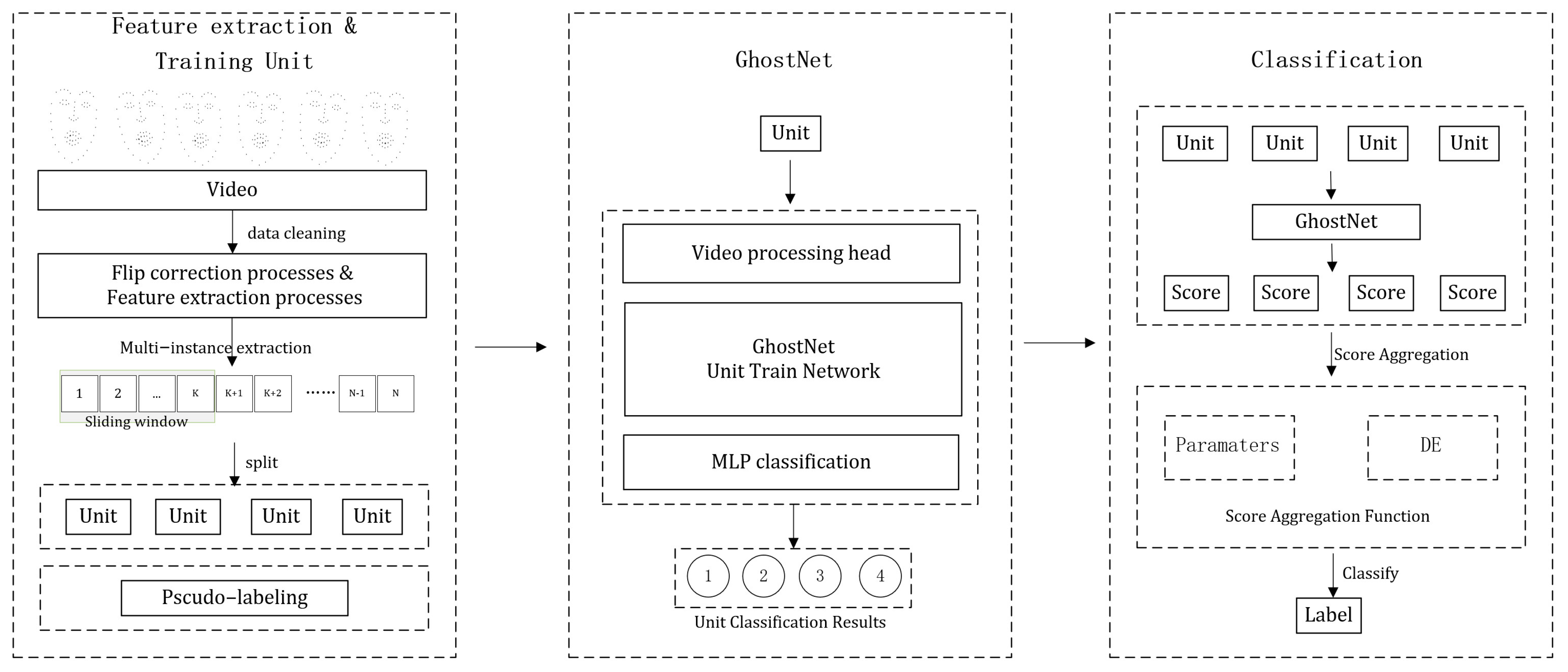
Figure 1. The framework of the proposed approach and its three phases.
Applsci 13 09230 g001
Figure 2. The face contains 68 landmarks.
Applsci 13 09230 g002
Figure 3. The rotational imaging model consists of two scenarios: (a) when the camera rotates around the optical axis during shooting, and (b) when the target rotates around the z-axis.
Applsci 13 09230 g003
Figure 4. The imaging model describes the motion of an object along the y-axis.
Applsci 13 09230 g004
Figure 5. The relationship between the target angle, image angle, and turnover angle during left and right deflections.
Applsci 13 09230 g005
Figure 6. The relationship between deflection angle and image angle.
Applsci 13 09230 g006
Figure 7. The process of feature extraction.
Applsci 13 09230 g007
Figure 8. The network architecture of GhostNet [31].
Applsci 13 09230 g008
Figure 9. ROC plot diagram for different model.
Applsci 13 09230 g009
Table 1. Angle of facial landmarker.
Sequence NumberCoordinate DefinitionMeaning
A 1 Ang(18,20,22)Curvature of the left eyelash
A 2 Ang(23,25,27)Curvature of the right eyelash
A 3 Ang(20,31,25)Grain lift 1
A 4 Ang(20,28,25)Grain lift 2
A 5 Ang(38,37,42)Degree of left eye corner opening
A 6 Ang(37,20,40)Degree of left eye squinting
A 7 Ang(47,46,45)Degree of right eye corner opening
A 8 Ang(43,25,46)Degree of right eye squinting
A 9 Ang(49,03,37)Degree of left cheek contraction
A 10 Ang(55,15,46)Degree of right cheek contraction
A 11 Ang(51,49,59)Degree of left outer lip opening
A 12 Ang(62,61,68)Degree of left inner lip opening
A 13 Ang(53,55,57)Degree of right outer lip opening
A 14 Ang(64,65,66)Degree of right inner lip opening
A 15 Ang(49,34,55)Degree of mouth opening
A 16 Ang(28,02,31)Nose wrinkle 1
A 17 Ang(28,16,31)Nose wrinkle 2
A 18 Ang(Le,31,Re)Upside down
A 19 Ang(01,30,03)Right deflection
A 20 Ang(17,30,15)Left deflection
Table 2. Parameters of GhostNet network.
InputOperator#Exp#OutSEStride
642 × 20Conv2d 3 × 3-84-2
322 × 84G-bneck1208411
322 × 84G-bneck2408402
162 × 84G-bneck2008401
162 × 84G-bneck1848401
162 × 84G-bneck48011211
162 × 112G-bneck67211211
162 × 112G-bneck67216012
82 × 160G-bneck96016001
82 × 160G-bneck96016011
82 × 160G-bneck96016001
82 × 160G-bneck96016011
82 × 160Conv2d 1 × 1-960-1
12 × 960AvgPool 8 × 8----
Table 3. This table presents the sample distribution of the DAIC-WOZ dataset [12].
DatasetsNon-DepressionDepression
Training set7730
Test set2312
Table 4. Comparison of the impact of video modality versus non-video modality data.
MethodsMPRF1
Manoret et al., 2021 [41]A0.640.910.75
Othmani et al., 2022 [14]A0.510.500.50
Rejaibi et al., 2022 [42]A0.690.350.46
Sun et al., 2019 [13]T0.670.500.57
Dinkel et al., 2020 [43]T0.850.830.84
Arioz et al., 2022 [44]A + T0.530.570.53
Lam et al., 2019 [45]A + T0.600.750.67
OursV0.770.830.80
Note: M = Modality in the table refers to the modality type. V = Visual refers to the visual modality data. A = Audio refers to the audio modality data. T = Text refers to the text modality data. + refers to the corresponding mixed multimodal.
Table 5. Comparison between the impact of the video modality itself and the data incorporating the video modality.
MethodsMPRF1
Wang et al., 2020 [28]V0.810.750.78
Song et al., 2018 [46]V0.640.580.61
Wei et al., 2022 [47]V + A + T0.890.570.70
Haque et al., 2018 [48]V + A + T0.710.830.77
Yang et al., 2021 [49]V + A + T0.710.550.63
OursV0.770.830.80
Table 6. Comparison of the effects of the vision itself.
FeatureMPRF1
GazeV0.850.500.63
PoseV0.720.660.69
2D landmarksV0.690.750.72
2D Landmarks + PoseV0.730.910.81
2D Landmarks + GazeV0.610.910.73
Ours AngleV0.770.830.80
Table 7. Ablation experiment for optimal sliding window.
Window_SizePRF1
180 s0.530.750.62
120 s0.770.830.80
60 s0.560.750.64
Disclaimer/Publisher’s Note: The statements, opinions and data contained in all publications are solely those of the individual author(s) and contributor(s) and not of MDPI and/or the editor(s). MDPI and/or the editor(s) disclaim responsibility for any injury to people or property resulting from any ideas, methods, instructions or products referred to in the content.