Fully Automated Dispensing System Based on Machine Vision

Abstract

To address the problems of low productivity and sizeable dispensing positioning errors in manual and semi-automatic dispensing processes in small- and medium-sized electronic enterprises, this study proposes a fully automatic dispensing method based on visual positioning with RJDNEL-type PCBs as the research object. The fully automatic dispensing system is constructed through the construction of a mechanical structure, the selection of optical equipment, and the debugging of the control system. The method is based on optical imaging technology. Firstly, the dispensing area is extracted through image preprocessing; then, the edge is detected by the Sobel operator, and the Hilditch operator optimizes the dispensing sharpness; then, the minimum outer rectangle algorithm is used to calculate the positioning information of the dispensing area by using the relationship between geometric transformations, which provides the database support for the realization of automatic dispensing; finally, the simulated annealing algorithm is adopted to optimize the dispensing path. Through the image acquisition matching experiments and positioning accuracy experimental analysis, it is concluded that the matching success rate is more than 99%, and the image positioning information repeated extraction accuracy error is less than 0.02 mm. Analysis of the total path of dispensing, as well as computing time, was performed as follows: for the complete dispensing process, 20 PCB boards were used; the path optimization of the dispensing path was reduced by 723.4 mm, and the dispensing efficiency was improved by 20% to 30%; after dispensing, the dispensing area measurement was performed on the PCB boards. PCB boards meet the quality requirements of dispensing, and the proposed method for meeting the quality of dispensing at the same time effectively improves the dispensing accuracy and efficiency.

1. Introduction

Increasing production demand promotes the rapid development of microelectronic devices, but many micro–nanodevices and microelectromechanical systems have not been practically used as products. This is because dispensing technology used in micro–nanosize encapsulation and assembly is one of the main obstacles, such as the size of the glue point, the amount of glue, and precision [1]. The traditional dispensing process and production mode have the shortcomings of low efficiency, high labor intensity, many human uncertainty influencing factors, unstable quality, etc. Therefore, traditional dispensing will be gradually eliminated in the progress of technology; the design and development of higher efficiency, higher precision, and lower-cost dispensing equipment are in line with the development of the times of research, with universal practical significance.

Machine vision systems have the advantages of high accuracy, speed, efficiency, and better reliability performance than manual vision systems [2,3,4]. The small circuit board dispensing system is no longer a simple dispensing module but a fusion and integration of a machine vision module, upper computer processing module and automatic control module, and other functional modules, and it has developed and grown due to its unique features and advantages; it has also become the leading technology for dispensing positioning and packaging of electronic products. Vision system-based dispensing products are applied to 40 to 50% of the objects concentrated in the field of electronic processing and the semiconductor industry, mainly in the United States, Switzerland, Japan, and other countries and regions where image processing technology is more developed [5]. Integrated automatic dispensing equipment is a mainstream direction of the production of dispensing machine apparatus systems.

Liu Ying et al. [6] proposed a new method based on a laser distance measurement sensor for high-precision alignment and an efficient dispensing method for millimeter objects, which is converted into increments of the images captured by the side cameras through the image Jacobi matrix. Even if the normal vector surface of the thin component is not perpendicular to the optical axis of the side camera, better measurement accuracy can be obtained. Based on the measurement results, the two components can be oriented and position-aligned with high accuracy. However, there is the drawback of being time-consuming. Zhang Xingwei et al. [7], based on the CycleGAN method for enhancing the dispensing image, effectively improve the problem of UV glue caused by the dispensing image showing low contrast, reduce the difficulty of visual detection, and effectively overcome the problem of blurred edges and low contrast. However, the success rate cannot fully meet the absolute accuracy requirements of product detection in actual industrial automated assembly lines. At the same time, in the actual industrial application environment, a lot of labor and material resources are usually required to obtain sufficient data samples. Nianfeng Wang et al. [8] designed a visual localization system for a dispensing robot based on a digital signal processor (DSP) to locate the position of feature points on the engine cover. The system corrected the original schematic trajectory in real time to maintain the accuracy of the gluing operation, but the dispensing efficiency needed to be improved. Cheng Fang et al. [9] addressed that the traditional dispensing machine is usually the manual input of the dispensing path under the circumstances, which leads to the limitation of dispensing accuracy. A vision system was designed to use the path identified by vision instead of manual human input. The precision of the dispensing machine can reach 0.016 mm, thus solving the problem of low precision and poor stability of open-loop control. Chih Hsing Chu et al. [10] proposed a Programming by Demonstration (PbD) interface in augmented reality for motion planning of a three-axis CNC dispensing machine. The interface helps human planners efficiently determine the dispenser’s motion during the planning task. The augmented reality application provides guidance information to the planner in a video of the real environment while guiding the machine to dispense glue to the workpiece in 3D space. Although the method saves 53.8% of the time compared to traditional methods, it cannot be fully automated and requires human integration.

However, in the field of small and microelectronic product packaging, due to the diverse dispensing of packaging products and models, packaging precision requirements, complex application environments, etc., the development of dispensing technology and equipment systems could be faster for small- and medium-sized enterprises. They are limited by cost and other reasons, or they could choose to use a lower degree of automation of semi-automatic dispensing equipment—or even manual operation—to complete production; to a large extent, this restricts the formation of an independent electronic product industry chain and supply.

The purpose of the research in this paper is to develop a machine vision-based high-precision and high-efficiency automatic dispensing system in order to solve the problems of small- and medium-sized enterprises, such as low production efficiency and dispensing positioning errors. An RJDNEL-type PCB board is the research object, which adopts machine vision technology and transmission and has an automatic control system. First of all, the composition of the various parts of the machine and the structure of the planning, the development of automatic dispensing platforms, and the utilization of machine vision are combined with the host computer. Then, images are collected in the host computer for processing, that is, image-processing algorithms are used. This paper uses Sobel operator edge detection, Hilditch operator optimization of the dispensing edge, and use of the minimum outer rectangle algorithm for the location of the dispensing area to extract information. Finally, the simulated annealing algorithm is used to plan the optimal point of the adhesive path. Compared with traditional dispensing equipment, this dramatically improves accuracy and efficiency.

2. Dispensing Positioning Information Extraction

The image processing and information extraction of the dispensing object is mainly done by image acquisition of the dispensing object, image processing such as graying of the PCB board to extract the dispensing object, shape-based template matching, edge optimization of the dispensing object, etc. Finally, the minimum outer rectangle algorithm is used to extract the aspect ratio, the area of the dispensing area, and the single dispensing area bit pose data. This time, MATLAB R2022b software is used for image extraction.

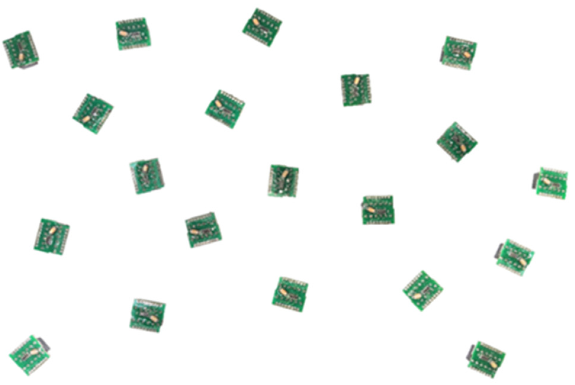
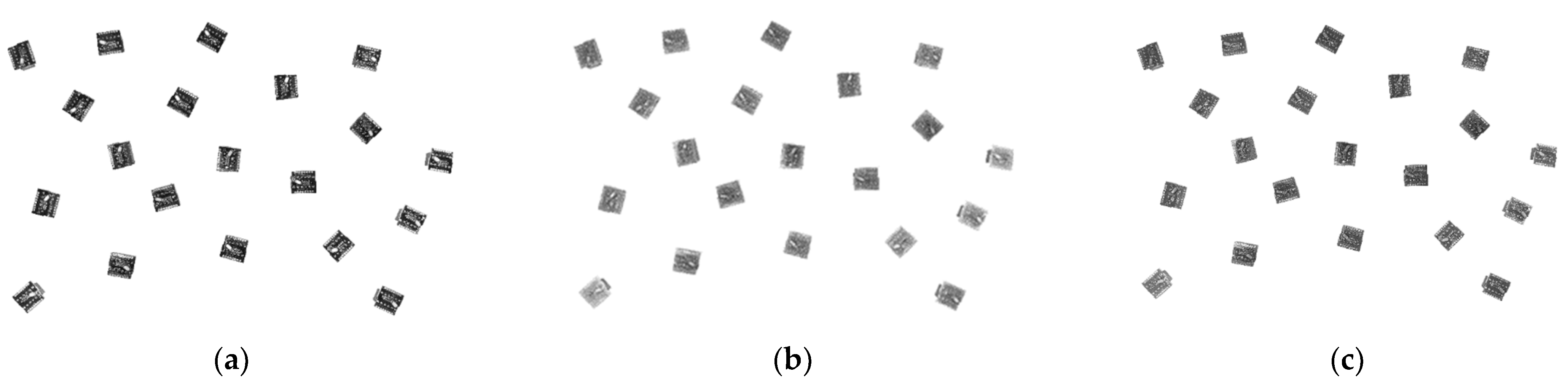
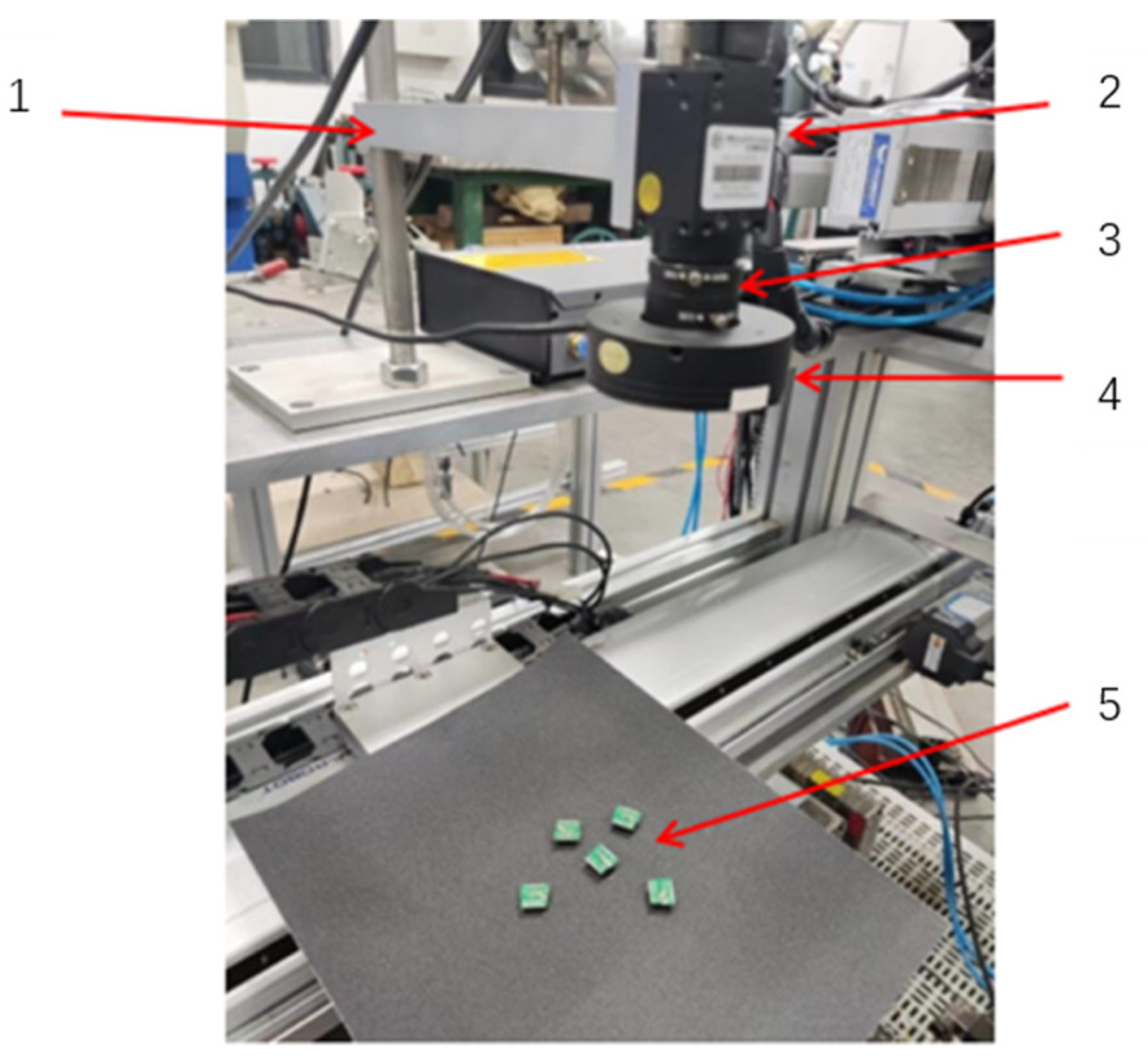
2.1. Dispensing Target Image Acquisition

This paper uses the human–computer interaction platform for image acquisition; the specific process is as follows: first install and configure the imaging device and acquire the image acquisition device, create a video input object, and then preview the acquisition of real-time images, and finally create the image acquisition object in the settings can be pre-set for the camera exposure, gain, etc., the acquisition PCB board is shown in Figure 1.

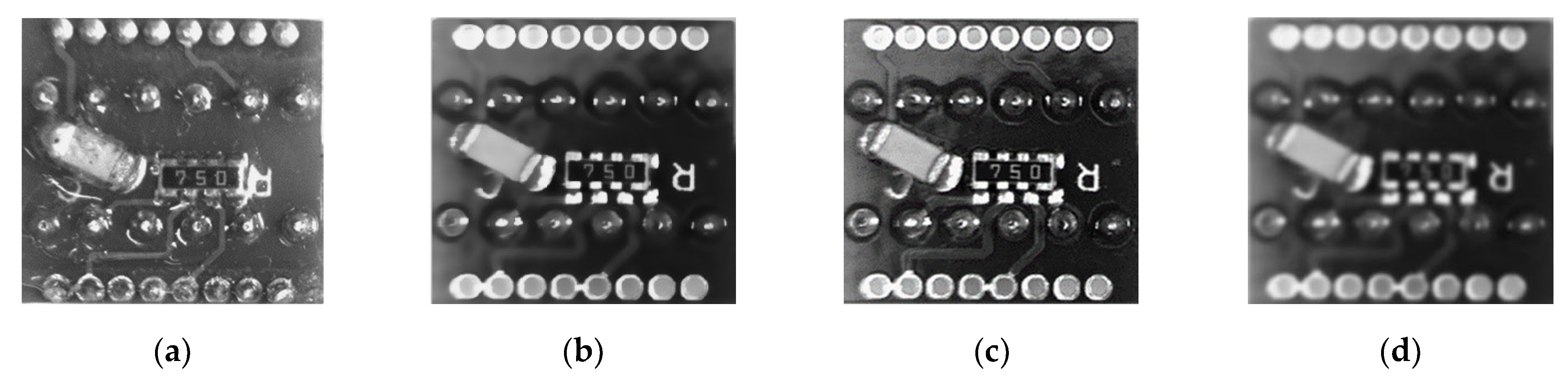
2.2. Image Processing of PCB Boards

Since the structure of the image features acquired through the camera is not obvious, there will be poor contrast, noise, etc., so it needs to be further processed through image processing, which is mainly through grayscale conversion, noise reduction, binarization, morphological operations, and the use of edge detection and optimization of the PCB board [11].

2.2.1. Grayscale Processing of PCB Boards

The acquired images have grayscale concentrated in a narrow range of areas due to various reasons, which causes the light and dark areas of the image to not stand out. Underexposure causes the image grayscale to be mainly concentrated in the low luminance range, while overexposure causes the grayscale to be mainly concentrated in the high luminance range. Improving image contrast requires equalizing the frequency at which each pixel appears. The essence of equalization is that any grayscale in the range of [0, 1] is evenly distributed within [0, 1] and the position of the coordinate points is guaranteed to be constant.

We set the input image grayscale distribution level $P_r\left(r\right), r\in \left[0, 1\right]$ and the output image grayscale distribution level $P_s\left(s\right), s\in \left[0, 1\right]$; in the definition of equalization, it is required that any s has $P_s\left(s\right)=1$. After the transformation of the elements of adjacent grayscale levels, the grayscale remains adjacent.

$$P_s\left(s\right)ds=P_r\left(r\right)dr .$$

(1)

Moreover, when $P_s\left(s\right)=1$, it follows that:

$$s={{\displaystyle \int }}_0^{s}dv={{\displaystyle \int }}_0^s{P}_s\left(v\right)dv={{\displaystyle \int }}_0^r{P}_r\left(w\right)dw .$$

(2)

The number of pixels accumulated from 0 to s in the gray value after the transformation equals the pixel value accumulated from 0 to r in the gray value before the transformation. At the same time, the image is channel decomposed and converted into three channels of RGB images, as shown in Figure 2, where a single-component method is used for the grayscale linear transformation, which is calculated as follows:

$$G\left(i, j\right)=W_R\times R\left(i, j\right)+W_G\times G\left(i, j\right)+W_B\times B\left(i, j\right) .$$

(3)

where $G\left(i, j\right)$ denotes the pixel value of the $\left(i, j\right)$ coordinate point after graying, and $R\left(i, j\right)$, $G\left(i, j\right)$, and $B\left(i, j\right)$ denote the red, green, and blue component values of this point, respectively. $W_R$, $W_G$, and $W_B$ denote the coefficients of the three components of the above-mentioned colors and satisfy $W_R+W_G+W_B=1$.

As can be seen from Figure 2, the contrast between the three RGB components and the background differs greatly, among which the R component of grayscale processing, as in Figure 2a, has a strong contrast between the dispensing area and the background, which can better identify the dispensing area. In summary, a single-component R map in grayscale processing is used as the image subsequent processing map.

2.2.2. Filtering of PCB Boards

In actual production, the image information captured by the process of camera acquisition and image transmission is particularly susceptible to contamination by noise, including pretzels (the most common), Gaussians, and pulses, which degrades and affects the image quality and increases and affects the difficulty of feature extraction of image information [12]. Therefore, the acquired images must be filtered for noise reduction.

In this paper, the single PCB board is filtered by mean filtering, median filtering, and Gaussian filtering in three ways, as shown in Figure 3.

Mean filtering is shown in Figure 3b; the noise in the image is reduced, but the image becomes blurred because the mean filter filters out the high-frequency components of the image, so the edges of the image are blurred (to remove a certain amount of pretzel noise, consider using median filtering). Median filtering is shown in Figure 3c; the noise in the figure is well smoothed, and it is not blurred too much as the mean. Gaussian filtering is shown in Figure 3d; Gaussian filtering is more complicated to handle, and the more low frequencies caused by the operation, the bigger the blur caused. To sum up, this paper finally selects the median filter of the 3 × 3 window according to the comparison of images after processing, and the whole image is bright and clear.

2.2.3. Binarization of the Dispensing Target

The grayscale histogram shows a large difference in grayscale between the dispensing object and the background image of the PCB board, which requires a lot of work to extract the object features; thus, the matching efficiency will be affected. In multi-objective acquisition matching, threshold segmentation removes the area outside the dispensing object and thus reduces the search area, i.e., to segment the dispensing object from the background. In this study, the Otsu algorithm is used for image segmentation: let an image have L different gray levels, and the number of pixels corresponding to a gray value of i is $n_i$, then the total number of pixels is obtained as:

$$N={\displaystyle \sum }_i^L=n_{i .}$$

(4)

The probability of each gray level is:

$$p_i=\frac{n_i}{N} .$$

(5)

The pixels in the image are divided into two groups according to the gray value using the threshold T. $C_0$ consists of pixels with a gray value within [$1, T$], and $C_1$ consists of pixels with a gray value between $\left[T+1, L\right]$.

It can be derived that the probability of generating $C_0$, $C_1,$ respectively, is:

$$w_0=\frac{{{\displaystyle \sum }}_{i=1}^T{n}_i}{N}={\displaystyle \sum }_{i=1}^T{p}_i .$$

(6)

$$w_1=\frac{{{\displaystyle \sum }}_{i=T+1}^L{n}_i}{N}=1-w_0 .$$

(7)

where the average grayscale of the $C_0$, $C_1$ group is:

$$u_0=\frac{{{\displaystyle \sum }}_{i=1}^T{n}_i\times i}{{{\displaystyle \sum }}_{i=1}^T{n}_i}=\frac{{{\displaystyle \sum }}_{i=1}^T{p}_i\times i}{w_0} .$$

(8)

$$u_1=\frac{{{\displaystyle \sum }}_{i=T+1}^T{n}_i\times i}{{{\displaystyle \sum }}_{i=T+1}^T{n}_i}=\frac{{{\displaystyle \sum }}_{i=T+1}^T{p}_i\times i}{w_1} .$$

(9)

The average grayscale of the whole image is:

$$u={{\displaystyle \sum }}_{i=1}^L{p}_i\times i .$$

(10)

where the grayscale average at a threshold value of T is:

$$u\left(T\right)={{\displaystyle \sum }}_{i=1}^T{p}_i\times i .$$

(11)

In summary, it can be seen that the sampled grayscale averages are:

$$u=u_0\times w_0+u_1\times w_0 .$$

(12)

Analogous variance:

$${\delta }^2=w_0{\left(u_0-u\right)}^2+w_1{\left(u_1-u_2\right)}^2=w_0{w}_1{\left(u_0-u_1\right)}^2$$

(13)

Then take a suitable value of T (1 < T < L) to make ${\delta }^2$ maximum, at which time T is the best threshold for the maximum interclass variance method to get the best segmentation effect.

Then Blob analysis with morphological processing, etc., is used to extract a single dispensing object, as shown in Figure 4.

The overall binarization diagram of 20 dispensing PCB boards is shown in Figure 5. The white area in the diagram is the dispensing area. Through the binarization segmentation process, each dispensing area is successfully segmented out and visible, laying the foundation for the edge extraction of the dispensing area in the later step.

2.3. Dispensing Region Edge Extraction and Refinement

2.3.1. Sobel Operator-Based Edge Extraction of the Dispensing Region

The Sobel operator is a gradient-based edge detection method mainly used for edge detection. Technically, it is a discrete difference operator, which is used to compute the grayscale approximation of the image luminance function. The convolution factor of the Sobel operator is two sets of 3 × 3 matrices (horizontal and vertical, respectively), and the whole image is convolved in a plane; that is, the horizontal and vertical luminance difference approximation can be found, respectively.

The image is weighted and averaged by the above 3 × 3 convolution template in two directions. Then the edge of the image is detected by the calculation method of first-order differentiation. Define the image function as $f\left(x, y\right)$, then its gradient $\mathsf{\nabla }f\left(x, y\right)$ at $\left(x, y\right)$ is a vector, defined as:

$$\mathsf{\nabla }f\left(x, y\right)=\left[\frac{G_x}{G_x}\right]={\left[\frac{\mathsf{\partial }f}{{\mathsf{\partial }}_x}\frac{\mathsf{\partial }f}{{\mathsf{\partial }}_y}\right]}^T .$$

(14)

where the magnitude and direction of the gradient $\mathsf{\nabla }f\left(x, y\right)$ are as in Equations (15) and (16):

$$\mathsf{\nabla }f\left(x, y\right)={\left[{\left(\frac{\mathsf{\partial }f}{{\mathsf{\partial }}_x}\right)}^2+{\left(\frac{\mathsf{\partial }f}{{\mathsf{\partial }}_y}\right)}^2\right]}^{\frac{1}{2}}$$

(15)

$$\alpha \left(x, y\right)=arctan\left[\frac{G_x}{G_y}\right] .$$

(16)

The specific steps of edge detection using the Sobel operator are:

• The 3 × 3 convolutional template is walked through the whole from top to bottom and from left to right on the collected dotted PCB template image, and the center point in the volume template corresponds to the pixel point in the image;
• The pixel value relative to each template composed of pixel points on the whole template image is derived by applying discrete convolution operation to each template;
• The maximum gradient value obtained from the horizontal and vertical convolution of the 3 × 3 convolutional template is substituted with the pixel value of the center pixel point;
• Finally, the appropriate threshold T is selected by many tests to carry out the recognition of the dotted area.

By collecting 20 randomly placed dispensing PCB boards, all of them can detect the edges of the dispensing area, as shown in Figure 6a. The detection at the marker is enlarged as shown in Figure 6b, with the edge detection on the dispensing object as shown in Figure 6c.

2.3.2. Hilditch Operator-Based Edge Refinement of the Dispensing Region

After the Sobel operator is used for edge detection of the dispensing area, some dispensing areas have redundant edge information and thick lines as shown in Figure 7a, which can lead to skewed matching and reduced matching accuracy. The Hilditch refinement operator determines whether a point in an image is a boundary or a connected point and removes the point if it is a boundary point. The application process is to iterate over each pixel of an image from the top left corner to the bottom right corner. Each iteration can remove the outermost layer of pixels from the image, and, finally, a line in the middle is left after the layers are peeled off to get the final refined image.

In this paper, we use the Hilditch refinement operator [13] to refine the edge of the dispensing object, which can optimize the edge lines in the thicker places and realize the obtained lines are smoother and the edge contour information is clearer, as shown in Figure 7b.

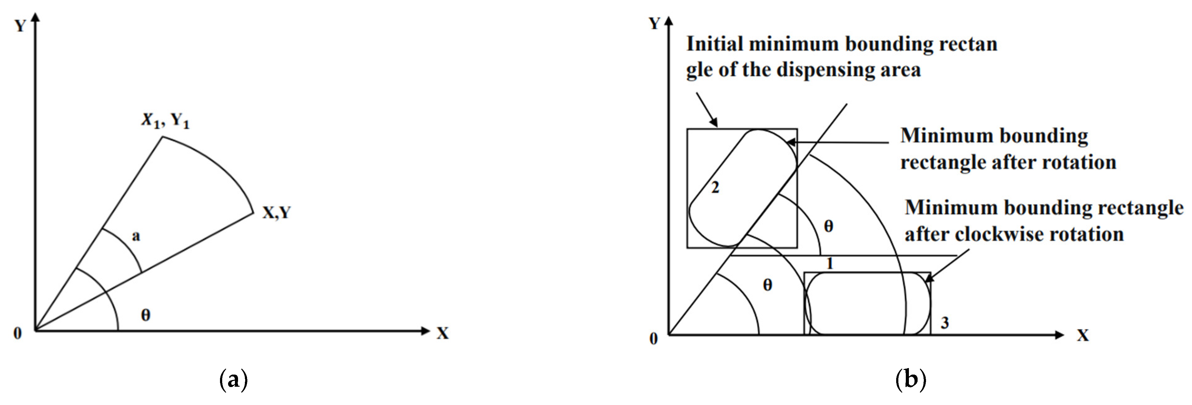
2.4. Extraction of Positioning Information Based on the Minimum Outer Rectangle Algorithm

2.4.1. Extracting the Aspect Ratio of the Dispensing Area

The shape of the dispensing area can be approximated as a rectangle, so the shape can be characterized quantitatively by the aspect ratio, which varies for different ranges of width-to-length ratios of the dispensing area. By finding the minimum external rectangle of the dispensing region, the length and width of the minimum external rectangle are used to approximate the maximum length and width of the equivalent dispensing region. Yuanwen Cao et al. [14] performed a comparative study of the shape characteristics of aggregate particles by optimizing the convex hull boundary rotation algorithm and verified the analysis by example to quickly calculate the particles’ flatness. According to their theory, the boundary rotation algorithm is used to calculate the minimum external rectangle for the dispensing region boundary in combination with this dispensing object, and its main steps include the following:

• Dispensing area boundary value determination.

The maximum value in the X-axis direction and the minimum value in the Y-axis direction of the dispensing boundary are used as the initial minimum external rectangle for the boundary rotation, and the area of the initial minimum external rectangle and the maximum and minimum coordinates on the boundary are recorded.

2.

Dispensing area boundary rotation.

Determine the angle ${\alpha }_i$ of each boundary line segment on the boundary of the dispensing area relative to the X direction. Calculate the angle of each boundary line segment on the boundary of the dispensing area relative to the X direction in the counterclockwise direction, and the rotation angle is calculated by the formula:

$${\theta }_i=arctan\left(\frac{y_{i+1}-y_i}{x_{i+1}-x_i}\right) .$$

(17)

where ${\theta }_i$ is the rotation angle of the ith line segment of the dispensing boundary, $x_i$ and $y_i$ represent the horizontal and vertical coordinates of the ith point of the dispensing area boundary.$x_{i+1}$ and $y_{i+1}$ are the horizontal and vertical coordinates of the ith + 1st point of the dispensing area boundary, respectively. The boundary of the dispensing area is rotated clockwise around the coordinate origin in the order of rotation angles ${\theta }_1, {\theta }_2, {\theta }_3, \dots , {\theta }_i.$ The basic principle is shown in Figure 8a. The point rotation transformation uses the same coordinate system, and the rotation coordinate formula is derived as:

$$x_i=r\cos {\alpha }_i .$$

(18)

$$y_i=r\sin {\alpha }_i .$$

(19)

$$x_i^{\prime }=r\cos \left({\alpha }_i-{\theta }_i\right)=r\cos {\alpha }_i\cos {\theta }_i+r\sin {\alpha }_i\sin {\theta }_i .$$

(20)

$$y_i^{\prime }=r\sin \left({\alpha }_i-{\theta }_i\right)=r\sin {\alpha }_i\cos {\theta }_i-r\cos {\alpha }_i\sin {\theta }_i .$$

(21)

$$x_i^{\prime }=\cos {\theta }_i{x}_i+\sin {\theta }_i{y}_i .$$

(22)

$$y_i^{\prime }=\cos {\theta }_i{y}_i-\sin {\theta }_i{x}_i .$$

(23)

$${\left(\begin{array}{cc}{x}_i^{\prime }& y_i^{\prime }\end{array}\right)}^T=\left(\begin{array}{cc}\cos {\theta }_i& \sin {\theta }_i\\ -\sin {\theta }_i& \cos {\theta }_i\end{array}\right)\left(\begin{array}{c}{x}_i\\ y_i\end{array}\right) .$$

(24)

$${\theta }_i=acrtan\left(\frac{y_{i+1}-y_i}{x_{i+1}-x_i}\right) .$$

(25)

where $x_i^{\prime }$ and $y_i^{\prime }$ represent the horizontal and vertical coordinates of the ith point on the boundary of the dispensing area after rotation, and ${\alpha }_i$ is the angle of the ith line segment of the boundary of the dispensing area relative to the X-axis direction.

The maximum value in the X-axis direction and the minimum value in the Y-axis direction of the rotated dispensing area boundary are used as the external rectangle after the boundary is rotated. The area of the rotated external rectangle is calculated and compared with the initial minimum external rectangle area. The four vertex coordinates and rotation angle of the external rectangle with the minimum external rectangle area are kept, and the external rectangle with the minimum area is displayed in the image. Then the boundary of the dispensing area with the external rectangle is reversed and rotated back with the same rotation angle, and its reversal coordinate formula is:

$${\left(\begin{array}{cc}{x}_i^{″}& y_i^{″}\end{array}\right)}^T=\left(\begin{array}{cc}\cos {\theta }_i& -\sin {\theta }_i\\ \sin {\theta }_i& \cos {\theta }_i\end{array}\right)\left(\begin{array}{c}{x}_i^{\prime }\\ y_i^{\prime }\end{array}\right) .$$

(26)

where $x_i^{″}$, $y_i^{″}$ are the horizontal and vertical coordinates of the ith point on the boundary of the dispensing area after reverse rotation, respectively.

Figure 8b is a schematic diagram of the rotation process of the dispensing region. The initial position of the dispensing region is at an angle of $\theta$ with the horizontal direction X-axis to determine the boundary value of the dispensing region. The black rectangle is the initial minimum external rectangle of the dispensing region, which will rotate the dispensing region around the coordinate origin in the clockwise direction to the horizontal position to find its external rectangle, and then counter-rotate the dispensing region to the initial position with the same rotation angle. Among them, the solid line No. 1 is the rotational trajectory line of the dispensing area, rectangle No. 3 is the external rectangle of the area after clockwise rotation, and rectangle No. 2 is the minimum external rectangle of the dispensing area after counter-rotation.

3.

Calculate the minimum external rectangle.

The boundary of the dispensing area is repeatedly rotated in the order of rotation angles ${\theta }_1, {\theta }_2, {\theta }_3, \cdots , {\theta }_i.$ If the area of the external rectangle obtained after rotation is smaller than the area of the previous external rectangle, the area of the current external rectangle, the four vertex coordinates, and the rotation angle will be kept until all the boundaries are rotated, where the rectangle with the smallest area is the smallest external rectangle, and the smallest external rectangle will be connected by the four vertex coordinates in turn. Figure 9 shows the minimum external rectangle of the dispensing area. Figure 9a shows the minimum external rectangle for the single dispensing area, and Figure 9b shows the minimum external rectangle for the multi-dispensing area.

2.4.2. Extracting the Area of the Dispensing Area

Extracting the area of the dispensing region is very important for the dispensing process and the selection of dispensing equipment, etc. The approximate capacity of the dispensing cartridge can be roughly deduced from the dispensing area, which helps a lot to improve the whole platform automation. The number of pixels in the dispensing area can be calculated using the region props function [14] in Matlab image processing technology. The image comprises individual pixel points, and the true area can be found based on the number of pixels by calculating the true area represented by each pixel point [15]. The calculation formula is:

$$S=\frac{S_0\times W_1}{W_0} .$$

(27)

where S₀ is the actual area of the reference, W₁ is the total number of pixels in the dispensing area, W₀ is the total number of pixels in the reference, and the number of pixels in the dispensing area and the reference is shown in Figure 10.

The actual area $S_0$ = 4 mm × 2 mm of the standard reference with pixel number $W_0$ = 2241 is shown on the left side of the figure, and the dispensing area with pixel number $W_1$ = 2210 is shown on the right side, so the actual area of the dispensing area can be found according to the formula. To further determine whether the area detected by the edge is the dispensing area, the area is determined according to the area. By comparing the aspect ratio and area of the target to be dispensed, which are measured in advance through the microscope, both are satisfied, and the aspect ratio is within 0.5~2 and the area is also within 2200~2300 pix, and the identified edge is retained; otherwise, it is removed.

2.4.3. Dispensing Area Center Coordinate Point Extraction

In extracting the aspect ratio of the dispensing area, $P_0\left(x_0, y_0\right)$, $P_1\left(x_1, y_1\right)$, $P_2\left(x_2, y_2\right),$ and $P_3\left(x_3, y_3\right)$ have been extracted as the four vertex coordinates of the minimum outside rectangle. As the extracted known quantity, the calculation of the center coordinate point $P_4\left(x_4, y_4\right)$ of the dispensing area is completed.

$$x_4=\frac{x_3-x_1}{2}=\frac{x_2-x_0}{2} .$$

(28)

$$y_4=\frac{y_3-y_1}{2}=\frac{y_2-y_0}{2} .$$

(29)

2.5. Dispensing Location Information Extraction Experiment

This topic is based on the design of a machine vision dispensing platform, the key role of its machine vision in the extraction of dispensing location information data—mainly through image acquisition, image processing, template matching, and creation—and other operations to achieve the extraction of dispensing point information data.

Five randomly selected PCB boards, as shown in Figure 11, are placed in the tray, and the whole dispensing tray is placed within the camera’s field of view and placed arbitrarily for position information extraction. Finally, by compiling the upper computer program, the matching score of the dispensing object target, the extraction of X/Y coordinate points, and the angle of random placement can be displayed. The coordinate information extraction for five PCB boards is shown in

Table 1. Dispensing area location information extraction for five PCBs.

Number	Dispensing Area Center Coordinate Point/Pixel	Dispensing Area/Pixel
1	(294, 235)	2215
2	(352, 708)	2235
3	(436, 483)	2218
4	(707, 282)	2230
5	(610, 413)	2228

.

3. Vision Dispensing Camera Calibration and Path Planning

3.1. Dispensing Vision System Hand-Eye Calibration

Proper calibration and alignment of the vision system are crucial to achieving accurate positioning. Surita Maini et al. [16] proposed a method for estimating the position and orientation of a camera that uses interest points in frames of a digital video and performs better than existing methods used for camera position estimation. Ashwani Kumar et al. [17,18] worked on methods for obtaining localization accuracy in urban scenes.

In the dispensing process, because the object information parameters collected by the camera cannot be directly applied to robot dispensing, it is necessary to carry out Eye-to-Hand calibration of the dispensing vision system camera. In machine vision, hand-eye calibration aims to obtain the relationship between the robotic arm coordinate system and the camera coordinate system, and finally convert the result of image acquisition and recognition into the robotic arms end coordinate system [19,20,21]. In this paper, the hand-eye calibration method of Eye to Hand is used for calibration. After the positioning information of the dispensing object is extracted, if the identified point coordinates are directly sent to the motion control, the dispensing will be carried out in the order of sending, which cannot ensure that the dispensing path is optimal; this requires the introduction of the path optimization algorithm, and then sending to the control system through the corresponding optimization algorithm after the optimization of the dispensing path is good. This can effectively improve dispensing efficiency.

3.2. Dispensing Motion Path Planning

In this section, the dispensing path planning method will be used to perform the dispensing path planning operation first, and then transfer the planned coordinate sequence to the motion control system of the pipette needle, to achieve a shorter dispensing path and improve the efficiency of the dispensing system.

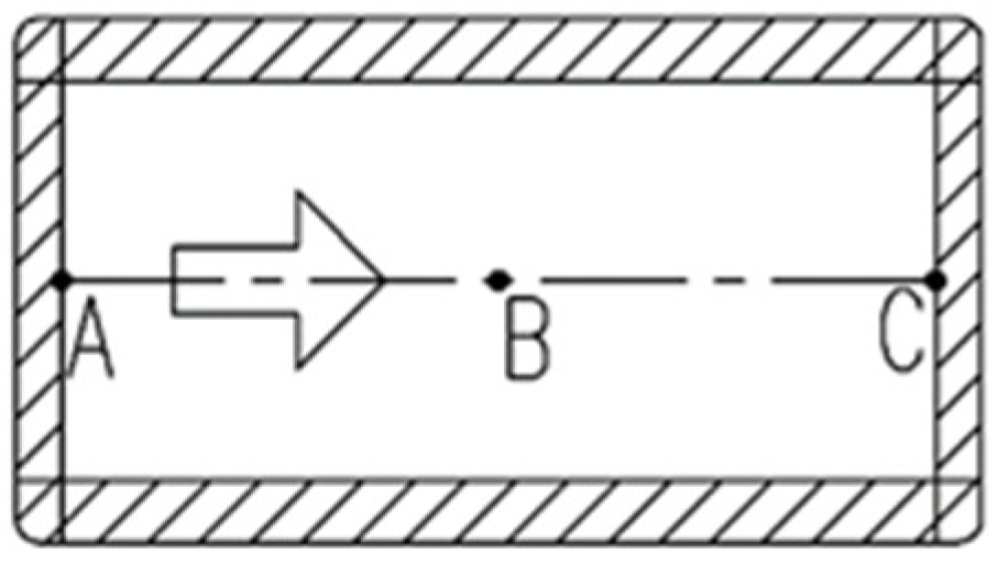
3.2.1. Dispensing Motion Path Analysis

In the process of the dispensing system for automatic continuous dispensing, to make the path taken by the dispensing needle in the dispensing system reach the optimal state, path planning is used to achieve a shorter dispensing path and improve the efficiency of the dispensing system, and also to analyze and study the dispensing path and dispensing posture of a single dispensing PCB board.

• Single dispensing object path analysis.

According to the dispensing process, the dispensing target is a capacitor of length × width (4 mm × 2 mm); the size sketch is shown in Figure 12, and the boundary chamfer is left with 0.25 mm margin at the upper and lower edges, i.e., $W_1$ = 3.5 mm, and 0.2 mm margin at the left and right edges, i.e., $W_2$= 1.6 mm. According to the above, the dispensing needle dispensing inner diameter ${\varphi }_1$ = 2.5 mm, and the constant spitting volume per second $\delta$ = 1 mL/s. We set the dispensing width $W_3$ = 2.5 mm, which in turn leads to linear dispensing on the dispensing target with the motion path shown in Figure 13, from point A to point B. And the moving speed $v_1$ during dispensing:

$$v_1=\frac{L-0.5}{t} .$$

(30)

where L is dispensing object length; according to the dispensing index requirements of each PCB board, dispensing time does not exceed 4 s, and both can be derived from $v_1=0.9 \mathrm{mm}/\mathrm{s}$.

2.

Analysis of single dispensing object dispensing direction and starting point.

As it is randomly placed in the PCB board code tray, this requires the pose analysis of the single object. This is mainly single target dispensing start position determination and path direction determination. A PCB board is randomly selected for analysis, as shown in Figure 14, and the coordinates of points $P_0, P_1, P_2,$ and $P_3$ are known to be $\left(x_0, y_0\right), \left(x_1, y_1\right), \left(x_2, y_2\right), \left(x_3, y_3\right)$ and the angle θ. The coordinates of the starting point A and the ending point C can be derived by the geometric operation of the coordinate points X/Y. The coordinates of the starting point A and the ending point C can be obtained by geometric operation of the coordinate points X/Y, and then linear interpolation can be used to realize the dispensing according to the single dispensing path.

3.

Multi-dispensing position path analysis.

Combined with the dispensing requirements of the subject, two dispensing paths were initially analyzed. The traditional dispensing path is shown in Figure 15a. Traditional dispensing is performed by transferring the randomly marked dispensing position collected by the camera to the dispensing controller directly through coordinate transformation for dispensing, and the dispensing sequence is as follows: the dispensing needle starts from the zero point, dispenses the first object first, runs back to the origin after dispensing is completed, corrects the coordinates, then runs to the second point for dispensing, and so on until the fifth point returns to the origin after dispensing is completed. The control of this dispensing method is relatively simple, and the home point is revised after dispensing is completed, which has a long-running time and cannot meet the efficiency requirements; the running track is complicated.

Figure 15b shows the dispensing sequence after the dispensing path optimization. The dispensing needle starts from the origin, runs to point 1 and then dispenses, and does not return to the origin after dispensing but goes directly to the target points such as 2 and 3, and finally returns to the origin after dispensing is completed. The whole dispensing path is clear and the dispensing efficiency can be greatly improved, after which the coordinate error can be revised to meet the accuracy requirements. Comparing the two path planning methods, the improvement meets the dispensing requirements simultaneously and satisfies the use of the path algorithm under the current general trend.

3.2.2. Modeling of Path Planning Based on Simulated Annealing Algorithm

The problem of the multi-dispensing position path can be analyzed as the dispensing head starting from the origin, passing through each dispensing center point position without repetition, and finally returning to the origin, which belongs to the traveling merchant problem [21,22].

Combining the characteristics of the dispensing system and the dispensing object in this paper, the simulated annealing algorithm is chosen to plan and solve the dispensing path. The physical principle corresponding to the use of an annealing-based algorithm is the Metropolis criterion [23,24], and the specific flow chart of the simulated annealing algorithm used for the dispensing path is shown in Figure 16.

Based on the simulated annealing algorithm process, the algorithm is analyzed: assuming that the $N_{ij}$ (i = 1, 2, …, M; j = 1, 2, …, P) matrix is the set of nodes in the dispensing path, and thus the total demand $T_j$ (j = 1, 2, …, P) in the j-direction can be calculated for the path in the M-direction, which can be found as $T_j=n_{j1}{r}_1+n_{j2}{r}_2+\dots +n_{jM}{r}_M$ as shown in Equation (31):

$$T_j=\left[\begin{array}{cccc}{N}_{11}& N_{12}& \cdots & N_{1M}\\ N_{21}& N_{22}& \cdots & N_{2M}\\ \cdots & \cdots & \cdots & \cdots \\ N_{p1}& N_{p2}& \cdots & N_{pM}\end{array}\right]\left[\begin{array}{c}{r}_1\\ r_2\\ \cdots \\ r_M\end{array}\right]={{\displaystyle \sum }}_{i=1}^M{n}_{ji}{r}_i$$

(31)

The ideal demand in direction j can be calculated by the above equation, and by the same token, the demand in direction j can be calculated for S positions as shown in Equation (32):

$$C_{js}=N_{j1}{x}_{1s}+N_{j2}{x}_{2s}+\cdots +N_{jM}{x}_{Ms}=\left[\begin{array}{cccc}{N}_{11}& N_{12}& \cdots & N_{1M}\\ N_{21}& N_{22}& \cdots & N_{2M}\\ \cdots & \cdots & \cdots & \cdots \\ N_{p1}& N_{p2}& \cdots & N_{pM}\end{array}\right]\left[\begin{array}{c}{x}_{1s}\\ x_{2s}\\ \cdots \\ x_{Ms}\end{array}\right]={\displaystyle \sum }_{i=1}^M{n}_{ji}{x}_{is .}$$

(32)

Since the direction of the path from a dispensing point is random, the direction of the dispensing path must be compared, and only through comparison can the path be better optimized:

$$E=Min\left(\left|C_{1js}\left(t\right)-C_{2js}\left(t\right)\right|\right) .$$

(33)

By using Equation (33), we can derive the first S(S = 1, 2, 3, …, P) positions of the direction j(1, 2, 3, …, P) in the total path planning in the total dispensing path direction, and then by using the squared sum of the deviation of the ideal usage and the actual usage, we can derive the objective function of the optimized direction consumption rate as Equation (34):

$$F=\min {{\displaystyle \sum }}_{r=1}^R{{\displaystyle \sum }}_{j=1}^P{(S\times \frac{{{\displaystyle \sum }}_{i=1}^M{n}_{ji}{r}_i}{{{\displaystyle \sum }}_{i=1}^M{r}_i}-{{\displaystyle \sum }}_{i=1}^M{N}_{ji}{x}_{is})}^2=\min {{\displaystyle \sum }}_{i=1}^R{{\displaystyle \sum }}_{j=1}^P{(S{d}_j-C_{js})}^2 .$$

(34)

The constraints in the equation include:

$${{\displaystyle \sum }}_{i=1}^M{x}_{is}=s, i=1, 2, \cdots , M;s=1, 2, \dots , R .$$

(35)

$$x_{is}-x_{i,s-1}\le 1, i=1, 2, \dots , M; s=1, 2, \dots , R .$$

(36)

$$x_{is}-x_{i,s-1}\ge 0, i=1, 2, \dots , M; s=1, 2, \dots , R .$$

(37)

$$0<x_{is}<r_i, i=1, 2, \dots , M; s=1, 2, \dots , R .$$

(38)

Thus, the optimal path space solution is finally determined:

$N_{ij}=\left[K_{p1}, T_{i1}, T_{d1};K_{p2}, T_{i2}, T_{d2}\right]$.

4. Automatic Dispensing Platform Experiment and Verification Analysis

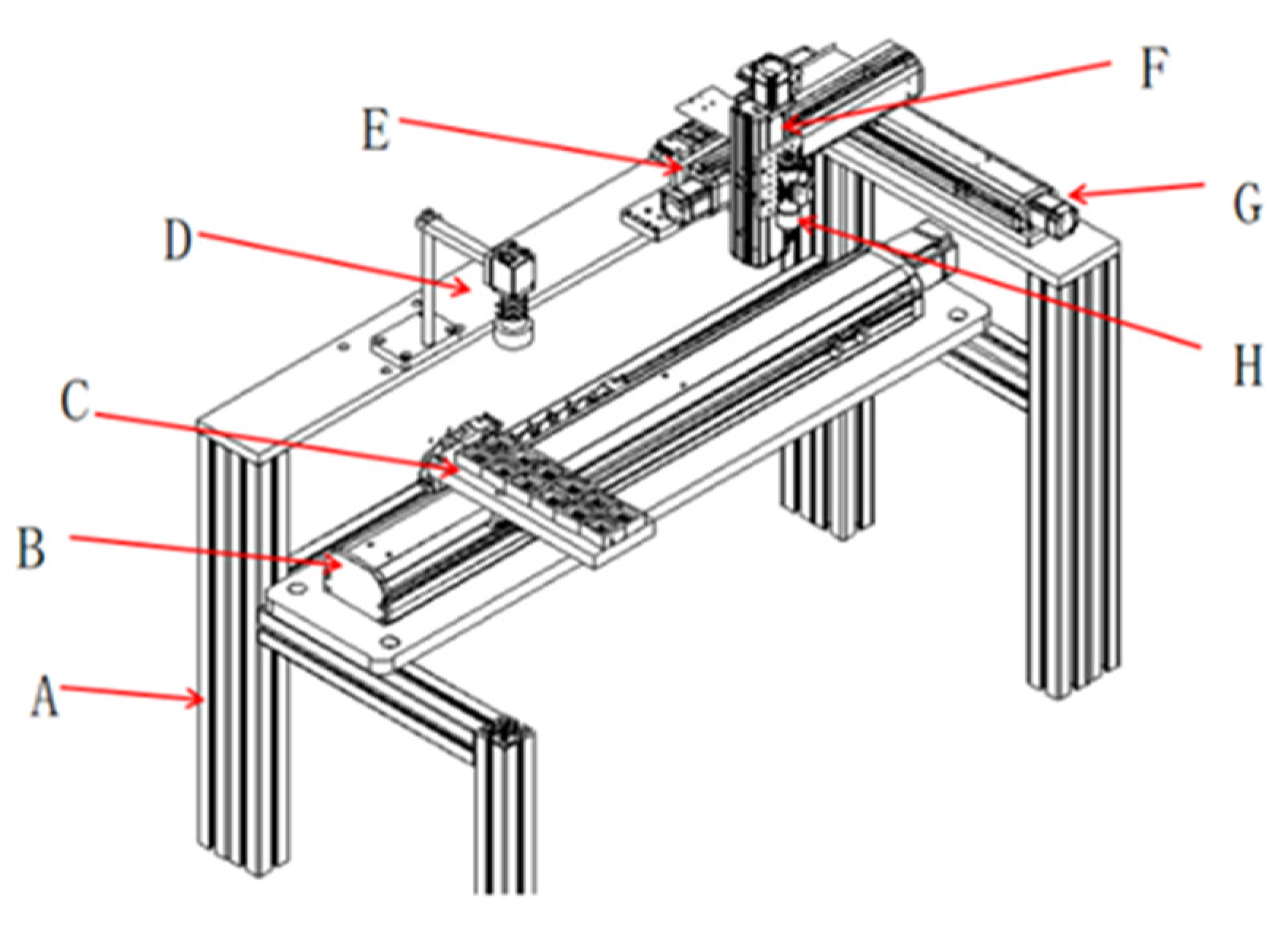
4.1. Dispensing Platform System

The dispensing platform mainly comprises three modules: mechanical structure module, machine vision system module, and control communication module.

4.1.1. Analysis of the Overall Mechanical Structure

According to the dispensing process shown in Figure 17, it is necessary to meet the movement of the PCB board on the conveyor mechanism, which can realize both camera acquisition and dispensing. The mechanical structure of the entire dispensing machine consists of the following parts: frame, conveyor, code plate, dispensing head, three-axis mechanical part, and vision acquisition system. The overall structural design dimensions are 1000 mm in length, 500 mm in width, and 870 mm in height. The design of the dispensing platform is shown in Figure 18.

The specific steps of each part are: first, after initialization of the device, the PCB board is loaded, the conveying mechanism (B) is conveyed to the vision system (D), the position sensor is triggered, the industrial camera is in image acquisition, and the upper computer receives signals for processing; second, the image processing and coordinate conversion is performed to determine the dispensing coordinates, and then the coordinate information is transmitted to the motion controller for compilation through signal transmission; third, the conveying mechanism conveys the code plate. The X-axis (E) and Y-axis (G) make a plane movement, and the dispensing head (H) moves up and down through the Z-axis (F), thus realizing PCB dispensing, and after dispensing is completed, the conveyor (B) moves to the next process. The whole mechanical structure has a small size, low cost, simple assembly and maintenance, and the three-axis mechanical structure is capable of linear interpolation motion.

4.1.2. Analysis of the Vision Dispensing System

The vision system mainly comprises three hardware parts: camera, lens, and light source. In this paper, the key hardware equipment of the micro dispensing visual identification system is specified as follows: an industrial camera with a resolution of 2448 × 2048 pixels is used, and the light source is an R70-36-20 type LED ring light source; the hardware will be used to build the dispensing visual platform, as shown in Figure 19.

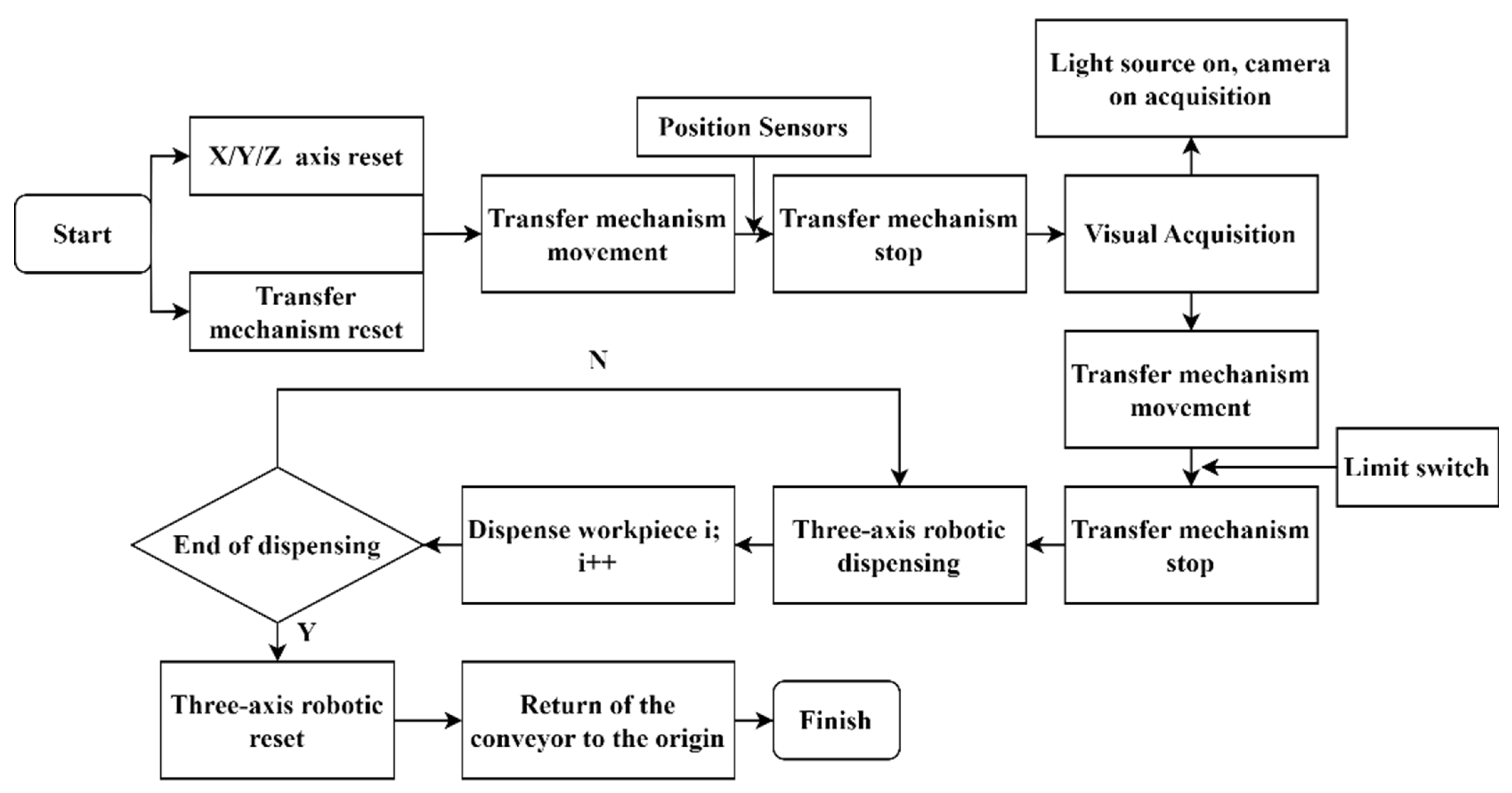
4.1.3. Overall Control Analysis

For subsequent software writing and hardware function upgrading, this paper uses an open control scheme with better compatibility, modularity, and secondary development [25]. In motion control, the motion control method that combines the motion control card and the PC side is used. The host computer, motion control card, servo driver, servo motor, I/O control module, and camera can be used as control system function modules to complete the control function.

This design uses an ECI1000 series motion control card (ECI1408 model), and PC is selected as the industrial control machine. The slot-type photoelectric sensor, light source controller, dispensing solenoid valve, X/Y/Z (three axes) mechanical axis limit module, emergency stop button, indicator light, buzzer, etc. are connected in a unified way, mainly through the digital output and input of the motion control card. The corresponding control signal is output after processing on the upper computer through the feedback signal of the sensor.

The complete dispensing experimental platform is built according to the overall design plan. The whole dispensing platform consists of the frame part, transfer mechanism, code plate and PCB board, three-axis mechanical module, dispensing vision part, and dispensing head and dispenser. The code plate is fixed on the transfer mechanism, the three-axis mechanical part and the vision part are mounted on the frame, the dispensing head is mounted on the Z-axis, and the code plate and PCB board are fixed on the transfer mechanism as shown in Figure 20.

After the whole dispensing platform is built, the overall mechanism runs smoothly, and the sequence of motion logic is correct. The overall actual operation flow is shown in Figure 21.

The main purpose of the control system is to dispense the capacitors on the PCB board and to meet the precision and efficiency of the dispensing. The entire dispensing platform can operate normally, but it is not a good explanation of the proposed design to improve the dispensing accuracy and efficiency, so the key functional modules are experimented with and verified to verify the key design content in the paper.

4.2. Hand-Eye Calibration Coordinate Data Extraction

The extracted coordinates in the figure are pixel coordinates, which cannot be used directly for dispensing path planning and need to be converted from pixel coordinates to actual dispensing coordinates by calibration conversion. The upper computer software performs the coordinate point conversion, and the conversion process is shown in Figure 22.

Before the coordinate point conversion, multiple pixel coordinates need to be extracted separately from the array of mechanical coordinates of the dispensing needle corresponding to them, substituted into the coordinate conversion formula with set camera parameters (internal and external parameters of the dispensing camera and distortion parameters, etc.), transposed along with other processing, and finally output the actual dispensing coordinate points. The experiment was tested with five PCB boards, and the collected pixel coordinate points were all converted as shown in

Table 2. Dispensing coordinate point conversion table.

Number	Pixel Coordinates (X/Y)	Actual Dispensing Position Coordinates (X/Y)
1	(706.8, 433.9)	(31, 19)
2	(1874.5, 548.2)	(82, 24)
3	(1095.4, 1120.1)	(48, 49)
4	(2098.5, 2056.5)	(92, 90)
5	(526.3, 1599.5)	(23, 70)

.

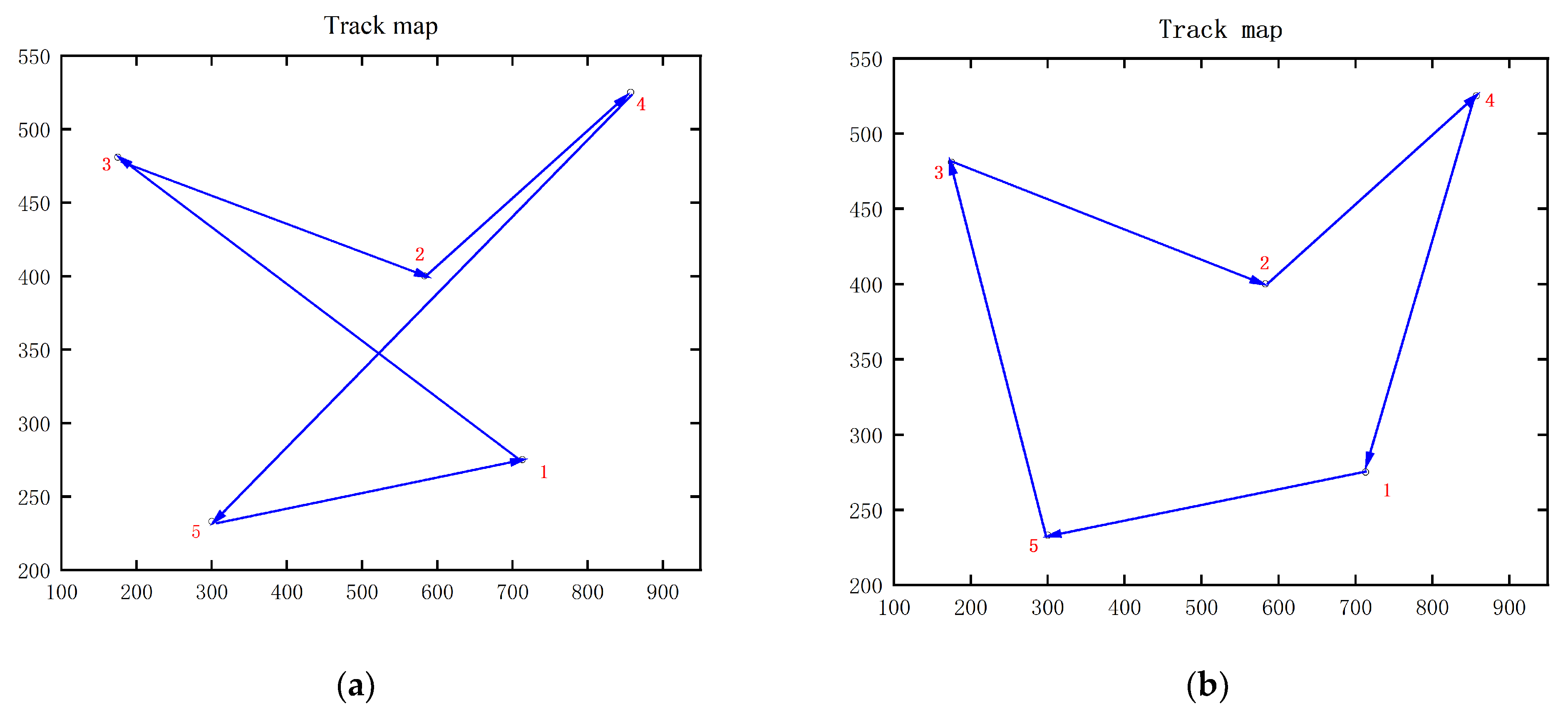
4.3. Experimental Verification of Multi-Point Glue Object Path Planning and Analysis

The conventional paths are arranged according to the calibration order of the image acquisition. The dispensing path planning is carried out directly after coordinating conversion, as shown in Figure 23a, and then the MATLAB software is used for effective path planning of the collected dispensing and positioning information. The initial condition parameters are set as shown in

Table 3. Simulated annealing algorithm parameter settings.

Parameters	Numerical Value
Initial temperature (t0)	1000
Cooling factor ($\Delta t$)	0.98
Number of iterations (N)	500
Temperature value after annealing (eps)	−11.28

. After the parameters are set, the coordinates of the center point of the area to be dispensed are obtained by visual recognition, and the program operation of path planning is completed. This experimental verification first uses the five-point location (five PCB boards) to verify the optimization of the path, as shown in Figure 23b.

From Figure 23, it can be seen that the five-point path planning does not differ much in the overall path length because the number of reference points is small, the use of a simulated annealing algorithm shows there is not much path change, the algorithm cannot converge well, and it does not reflect the advantages of optimization. Before and after the path optimization can only be seen more clearly in the figure, but its further depth of more points for dispensing has a good reference value.

Based on the 5-point path optimization, to increase the dispensing efficiency and further verify the optimization of this algorithm on the dispensing path, 20 points (20 PCBs) are used for experimental verification of the traditional dispensing path and the optimized path length comparison, as shown in Figure 24 for the 20-point traditional path planning diagram.

The optimized dispensing path is shown in Figure 25, combining image acquisition recognition and path planning.

According to the calculation of the paths optimized by the traditional path and the simulation algorithm, it is obvious that: the traditional dispensing path is messy, and the paths repeat alternately, with a total path of 1670.2 mm and a path planning time of 4.3 s; after the dispensing path optimization, the dispensing trajectory is clear and definite, with a total path of 946.8 mm and a path planning time of 2.3 s. It can be seen that the difference between the paths before and after the optimization is obvious, and the optimized path is 723.4 mm less than the conventional dispensing path, which shows that path optimization has a positive effect on improving the dispensing efficiency.

The accuracy of data extraction is related to the number of experimental validations; this experiment uses a total of 20 PCB boards placed randomly, and the path based on the simulated annealing algorithm is collected 30 times in three groups. Each group will be aggregated to eliminate the maximum value and minimum value, and the average value will be taken for comparison, as shown in

Table 4. Simulated annealing algorithm for path length extraction.

Group	$\mathbf{Conventional} \mathbf{Dispensing} \mathbf{Path} \mathbf{Length} \overline{{\mathit{L}}_1} \left(\mathbf{mm}\right)$	$\mathbf{Optimized} \mathbf{Dispensing} \mathbf{Path} \mathbf{Length} \overline{{\mathit{L}}_2} \left(\mathbf{mm}\right)$
1	1654.9	940.1
2	1713.4	959.8
3	1707.4	949.2

. The dispensing speed (3.5 mm/s) is the same, so it can be calculated that the dispensing time used after the path optimization is shortened, thus calculating a significant increase in dispensing efficiency.

4.4. Image Acquisition Recognition and Positioning Accuracy Experiment

The dispensing object is small, and manual dispensing and traditional dispensing cannot very well guarantee accuracy; to improve the dispensing accuracy, machine vision is used for image acquisition processing. For this purpose, the image acquisition experiment is done on the physical dispensing platform, where the PCB board is placed in the code tray for image acquisition, and the upper computer is compiled to display the number of the dispensing PCB board in the code tray in real time. Among them, image acquisition, image processing, image template matching, and other operations can be completed in the human–computer interaction interface of the upper computer, and the XY pixel coordinates and angle values of the center point of the dispensing area can be displayed in the data display area.

The image acquisition is the pre-work for the subsequent image processing and matching. The following experiments are conducted to match and locate the templates from the image acquisition, then the matching rate data and the positioning accuracy error are obtained.

1.

Localization information extraction experiment

The experiment selected 120 RJDNEL-type PCB boards, divided into five groups for the positioning information extraction test; the recognition results are shown in

Table 5. Positioning information extraction rate.

Experiment Serial Number	Total Number of PCB Boards/Block	Number of Correct Extractions/Block	Withdrawal Time/ms	Correct Extraction Rate
1	120	120	815	100%
2	120	120	820	100%
3	120	120	765	100%
4	120	119	910	99.2%
5	120	120	620	100%

. Analyzing the extraction test results, it can be concluded that 600 PCB boards correctly extracted 599 pieces, matching the correct rate above 99%. After repeated analysis of the test, one of the unsuccessful matches is due to the presence of edge-breaking missing PCB boards, not a defect in the extraction algorithm.

2.

Image recognition coordinate position accuracy error analysis.

In image acquisition, if the positioning coordinate points identified from each image differ greatly, this will lead to inaccurate dispensing in the subsequent actual dispensing process, which requires repeated identification and positioning test analysis for a certain position.

When doing the repeatability test, the standard deviation of the set of measured values represents the accuracy of the measured values [26]. This experimental theory uses the standard deviation as a quantitative criterion for the accuracy of repeatedly extracting the positioning coordinate points, and the experimental steps are as follows:

• The experiment randomly selects two PCBs into groups A and B.
• On the PCB board in group A, the collected image is pre-processed by grayscaling, filtering, binarization, etc., and then the edge extraction and refinement of the PCB board dispensing area are carried out. Finally, the coordinates of the center point of the dispensing area are repeatedly collected and extracted 10 times based on the minimum outer rectangle algorithm. The extracted coordinates are read out as (X₁, Y₁).
• Repeat the experimental steps in group B to obtain (X₂, Y₂).
• Calculate u(p) · X₁, u(p) · Y₁, u(p) · X₁₂, and u(p) · Y₂ by repeating the experimental standard deviation.

The details of analysis of the obtained repeat extraction coordinates are shown in

Table 6. Image acquisition to locate coordinate points.

Location	X1	Y1	X2	Y2
1	236.32	658.49	845.69	759.15
2	236.35	658.30	845.33	759.58
3	236.58	658.98	845.85	759.37
4	236.40	658.11	845.08	759.88
5	236.38	658.67	845.92	759.02
6	236.60	658.32	845.51	759.88
7	236.51	658.88	845.67	759.63
8	236.60	658.04	845.96	759.56
9	236.47	658.25	845.10	759.37
10	236.52	658.59	845.94	759.69

. The duplicate experimental standard deviation can be calculated according to Formulas (39) and (40) to calculate the duplicate position error.

$$\overline{p}=\frac{1}{n}{\displaystyle \sum }_{i=1}^n{p}_i .$$

(39)

$$u\left(p\right)=\sqrt{{{\displaystyle \sum }}_{i=1}^n\frac{{\left(p_i-p\right)}^2}{n}}$$

(40)

where $p_i$—data of the ith test; $u\left(p\right)$—repeatability test error.

Using the test that was used to analyze image recognition positioning accuracy error, the coordinate position of the center of the PCB board is derived as the alignment point, and the coordinates of the center point position of the dispensing area are extracted through the camera acquisition and processing image. According to multiple sets of repeated experiments, Formulas (39) and (40) with the data in the table can be calculated as follows: $u\left(p\right)X_1=0.014 \mathrm{mm}$; $u\left(p\right)Y_1=0.011 \mathrm{mm}$; $u\left(p\right)X_2=0.012 \mathrm{mm}$; and $u\left(p\right)Y_1=0.013 \mathrm{mm}$. According to the repeated test calculation analysis, the repeatedly extracted image coordinates error does not exceed 0.02 mm, which meets the design requirements.

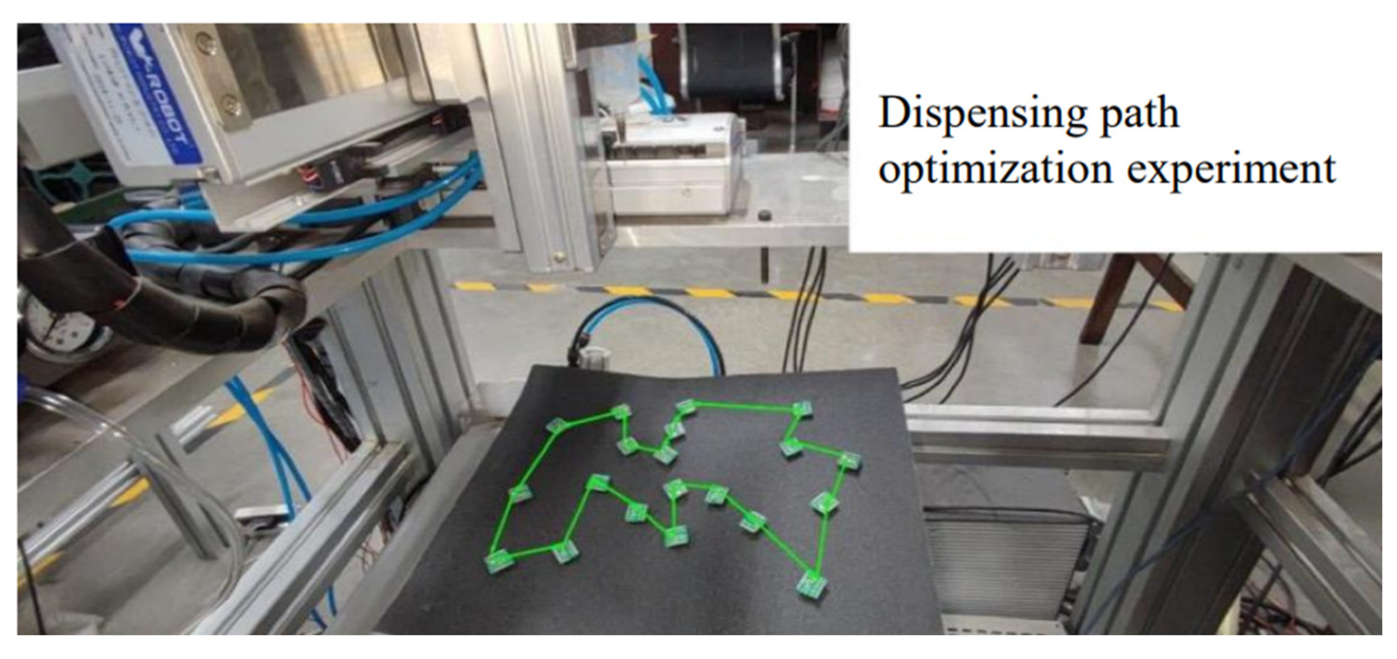
4.5. Path Planning Experiment and Verification

The experiment uses 20 pieces of dispensing PCB boards for experiments, randomly placed in the code plate for dispensing; the physical diagram is shown in Figure 26. The diagram is marked with the dispensing needle movement trajectory. At the same time, through the compilation of the upper computer, to complete the dispensing path optimization before and after the path, planning time, total travel and path real-time display of dispensing are determined.

In the path optimization above, a theoretical efficiency study was done before and after the dispensing path optimization, and here a comparative experiment is used to verify the dispensing time comparison before and after the dispensing path optimization, with the parameters set as shown in

Table 7. Path optimization experimental predicate parameter setting.

Category	Dispensing Operation Speed (mm/s)	Gum Spitting Volume (mL/s)	Number of Dispensing at a Time	Number of Groups
Parameters	1	1	20	5

.

Specific experimental methods are as follows:

• Set up five groups; each group chooses 20 PCB boards randomly placed, and the position of the PCB boards placed between different groups cannot be the same.
• Start timing from dispensing; when the dispensing is finished for the last PCB board, end the timing.
• Record the time for dispensing before and after the path optimization is carried out. The final experiment can be derived from the dispensing time of different groups, as shown in

  Table 8. Movement timetable before and after dispensing path optimization.

  Group	Number of Dispensing	Traditional Dispensing Is Time-Consuming/s	Optimized Dispensing Time/s	Efficiency Improvement Percentage
  1	20	429.4	297.6	30.7%
  2	20	420.3	298	29.1%
  3	20	397.6	295.1	25.8%
  4	20	374	293.6	21.5%
  5	20	396.4	298.1	24.8%

  . According to the above table, it can be concluded that the traditional dispensing path has a long dispensing time. After the path optimization, the dispensing efficiency improved by 20~30%.

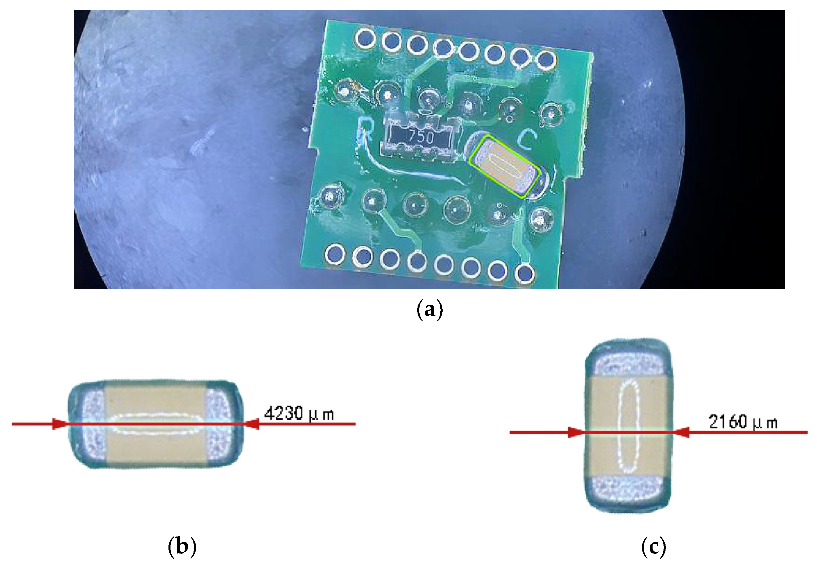
4.6. Dispensing Quality Testing Experiment

The purpose of construction of the entire dispensing platform is to carry out the dispensing, and whether the final dispensing out of the dispensing area meets the requirements (according to the quality inspection requirements of an electronics factory, a dispensing package accuracy of ±0.5 mm is required) is crucial. This experiment is the final dispensing quality verification experiment; the same irregular placement of the selection of 20 PCB boards was used, strictly using the process requirements for dispensing and the path based on the simulated annealing algorithm to optimize the dispensing path. Among them, the visual recognition system performs image acquisition processing and dispensing, and coordinate point extraction and transformation after 217.6 ms. The identified 20 points are shown in

Table 9. Figure 27: Extraction of information on the location to be dispensed.

Number	Image Acquisition Dispensing Coordinates	Angle	Actual Dispensing Coordinates	Dispensing Area/Pixel
1	(629.28, 713.64)	135.6	(27.6, 31.3)	2236
2	(1999.52, 1128.5)	165.2	(87.7, 49.5)	2245
3	(1108.04, 1598.28)	36.2	(48.6, 70.1)	2231
4	(264.48, 1550.5)	64.8	(11.6, 68)	2229
5	(2186.52, 579.12)	95.6	(95.9, 25.4)	2236
6	(1374.84, 1903.8)	308.9	(60.3, 83.5)	2227
7	(2031.04, 2197.92)	225.8	(88.8, 96.4)	2239
8	(642.96, 2008.68)	294.3	(28.2, 88.1)	2236
9	(948.48, 2058.84)	10.8	(41.6, 90.3)	2234
10	(2243.52, 2496.6)	302.2	(98.4, 109.5)	2225
11	(1051.08, 2421.36)	260.5	(46.1, 106.2)	2226
12	(836.76, 446.88)	159.7	(36.7, 19.6)	2227
13	(1942.56, 2118.13)	122.3	(85.2, 92.9)	2236
14	(978.12, 1459.2)	231.9	(42.9, 64.1)	2234
15	(585.96, 1146.84)	56.2	(25.7, 50.3)	2238
16	(565.44, 937.08)	78.3	(24.8, 41.1)	2229
17	(2268.6, 884.64)	170.8	(99.5, 38.8)	2237
18	(563.16, 1422.72)	264.9	(24.7, 62.4)	2231
19	(2154.6, 1561.9)	320.5	(94.5, 68.5)	2228
20	(886.92, 1694.06)	83.7	(38.9, 74.3)	2233

, before and after the transformation position information. The conveyor mechanism takes 7 s in motion from entering the dispensing platform to resetting after dispensing is completed.

The dispensing quality experiment uses a simulated annealing algorithm based on path planning; after 0.61 s to complete the entire path planning, the robot dispensing path was determined, as shown in Figure 27a. Then the planned dispensing path information is transmitted to the control system of dispensing after 109 s to complete the dispensing of 20 PCB boards; the average dispensing time of each PCB board is 4 s, while the dispensing platform is derived in 20 detailed enlargements of a PCB board. Dispensing quality results are shown in Figure 27. After testing, the general shape of the dispensing area is rectangular; the longest side is about 4400 μm, the shortest is about 4100 μm, the widest side is about 2300 μm, and the narrowest is about 2100 μm. All meet the dispensing accuracy requirements. The overall dispensing quality of the PCB board is good.

The information on the 20 dispensing positions is extracted from Figure 27 and the converted coordinates are shown in Table 9.

5. Discussion and Conclusions

This study combines the actual process requirements and process flow of small- and medium-sized enterprise factories. It proposes a fully automated dispensing system based on visual positioning to improve the automation, productivity, and product dispensing accuracy of dispensing equipment in small- and medium-sized enterprises, in response to the problems of low efficiency and unstable quality that exist in traditional dispensing processes and production modes. The research content of this paper is as follows:

• Firstly, the collected PCB images are preprocessed through grayscale processing, median filtering, and binarization. The dispensing area is extracted, the edges of the dispensing area are extracted by using the Sobel edge detection operator, the extracted edges are operated by using the Hilditch algorithm, and, finally, the center coordinates point, angle, and area of the dispensing area are extracted by using the minimum outer rectangle algorithm.
• The pixel coordinates after image processing are converted to the actual dispensing coordinates of the dispensing needle using hand-eye calibration. Analysis of the single PCB board dispensing path and dispensing direction, the overall path planning for 20 PCB boards, and the use of MATLAB software through the simulated annealing algorithm based on the optimization of the dispensing path were compared with the traditional dispensing path; the optimized total length of the dispensing path and the running time have been significantly reduced.
• For the overall program design, the dispensing experimental platform was constructed according to the design of the actual dispensing experiments. For the complete dispensing process, 20 PCB boards were used. For the host computer, image acquisition processing and coordinate conversion total time was 217.6 ms; from the first board to the last board, dispensing was completed in a time of 109 s. The entire dispensing platform total time was 126.8 s. Finally, dispensing was completed, and the dispensing area measurement was performed. Dispensing package accuracy was within ±0.5 mm; the optimized dispensing efficiency was improved. After optimization, the dispensing efficiency was improved by 20~30%.

In summary, the design of the fully automated dispensing platform meets the practical requirements for accuracy, efficiency, and platform automation and integration.

References

1. Liu, H.; Chen, X.; Sun, X.; Gao, Q.; Qiao, K. A pL-fL grade micro-dispensing by pipetting needle glue liquid transfer. AIP Adv. 2021, 11, 065119. [Google Scholar] [CrossRef]
2. Zha, G.F. Research on Dispensing Defect Based on Machine Vision. Master’s Thesis, HITSZ, Shenzhen, China, 2020. [Google Scholar] [CrossRef]
3. Nelson, A. Machine Vision Trends for Today’s Industrial Age. Quality 2020, 59, 26VS–29VS. [Google Scholar]
4. Scimeca, D. Machine vision’s hottest technologies and most popular applications. Vis. Syst. Des. 2021, 26, 10–12. [Google Scholar]
5. Wu, X.; Song, J. Research on visual detection and control system of three axis servo dispensing machine. Mach. Des. Manuf. 2020, 5, 237–240. [Google Scholar] [CrossRef]
6. Li, Y.; Zhang, D.; Xu, D. High precision assembly and efficient dispensing approaches for millimeter objects. Int. J. Adv. Robot. Syst. 2019, 16, 1729881419857393. [Google Scholar] [CrossRef]
7. Xing-Wei, Z.; Ke, Z.; Xie, L.-W.; Yong-Jie, Z.; Xin-Jian, L. An Enhancement and Detection Method for a Glue Dispensing Image Based on the CycleGAN Model. IEEE Access 2022, 10, 92036–92047. [Google Scholar] [CrossRef]
8. Wang, N.; Liu, J.; Wei, S.; Zhang, X. A Vision Location System Design of Glue Dispensing Robot. In Intelligent Robotics and Applications; Springer: Cham, Switzerland, 2015. [Google Scholar] [CrossRef]
9. Cheng, F.; Zhang, X.; Zhang, J.S. A positioning system for dispensing machine based on machine-vision. Mach. Des. Manuf. 2013, 3, 101–104. [Google Scholar] [CrossRef]
10. Chu, C.H.; Liu, Y.W.; Li, P.C.; Huang, L.C.; Luh, Y.P. Programming by Demonstration in Augmented Reality for the Motion Planning of a Three-Axis CNC Dispenser. Int. J. Precis. Eng. Manuf.-Green Technol. 2020, 7, 987–995. [Google Scholar] [CrossRef]
11. Mao, L.; Lian, W.H.; Fan, Z.Q.; Zhu, L.; Hu, J.W. Overview of digital image processing algorithms. Sci. Technol. Innov. 2020, 19, 29–30. [Google Scholar] [CrossRef]
12. Movafeghi, A.; Yahaghi, E.; Mirzapour, M.; ShayganFar, P. Defect Measurement in Welded Objects by Radiography Testing and Chambolle’s Image Processing Method. J. Nondestruct. Eval. 2021, 40, 49. [Google Scholar] [CrossRef]
13. You, S.; Zhang, H.; Zhou, Y.L.; Zhang, X.L. Repair of center lines’s break point of weld structure light based on hilditch algorithm. Hot Work. Technol. 2020, 49, 134–138+145. [Google Scholar] [CrossRef]
14. Cao, Y.W.; Yang, G.L.; Zhang, Y.Y.; Wang, R.J.; Cheng, Z.H. Rapid evaluation method of shape characteristics of aggregate particle based on the minimum outer rectangle. J. Chongqing Jiaotong Univ. (Nat. Sci.) 2019, 38, 61–65. [Google Scholar]
15. Wang, D.; Zhang, J.X.; Fan, J.; Zhai, X.L.; Dong, L.; Pei, W.X.; Wang, J.J. Evaluation method of commodity specification grade of lycii fructus based on image processing technology. Mod. Tradit. Chin. Med. Mater. Medica-World Sci. Technol. 2020, 22, 2817–2823. [Google Scholar]
16. Maini, S.; Aggarwal, A.K. Camera Position Estimation using 2D Image Dataset. Int. J. Innov. Eng. Technol. 2018, 10, 199–203. [Google Scholar]
17. Kumar, A.; Ikeuchi, K.; Sato, Y.; Oishi, T.; Ono, S. Improving gps position accuracy by identification of reflected gps signals using range data for modeling of urban structures. Prod. Res. 2014, 66, 101–107. [Google Scholar] [CrossRef]
18. Kumar, A.; Banno, A.; Ono, S.; Oishi, T.; Ikeuchi, K. Global Coordinate Adjustment of the 3D Survey Models under Unstable GPS Condition. Seisan Kenkyu 2013, 65, 91–95. [Google Scholar] [CrossRef]
19. Li, C.C. Study and Realization of Camera Calibration Technology in Machine Vision. Master’s Thesis, NUAA, Nanjing, China, 2009. [Google Scholar]
20. Zhang, Y.; Qi, J. Research on vision calibration method of large field view based on halcon. Mech. Electr. Eng. Technol. 2019, 48, 1–3. [Google Scholar]
21. Bao, Q. A hybrid genetic simulated annealing algorithm for solving the travel quotient problem. China Storage Transp. 2021, 11, 204–205. [Google Scholar] [CrossRef]
22. Graczyk, J.; Mihalache, N. Optimal bounds for the analytical traveling salesman problem. J. Math. Anal. Appl. 2022, 507, 125811. [Google Scholar] [CrossRef]
23. Gao, J.; Ren, Y.M. Simulated annealing based algorithm for solving combinatorial optimization problems. Sci-Tech Dev. Enterp. 2021, 5, 66–68. [Google Scholar]
24. Fan, W.P. Particle Swarm Optimization Algorithm and Its Application in Fuzzy Clustering ai Gorithm. Master’s Thesis, Lanzhou Jiaotong University, Lanzhou, China, 2021. [Google Scholar] [CrossRef]
25. Hu, C.Z.; Zhou, J.L. Design of Multi Axis Motion Controller Based on STM32 + FPGA. Mach. Tool Hydraul. 2021, 49, 82–86. [Google Scholar]
26. Sun, X.S.; Wang, S. Comparison of σ estimators in mean—Standard deviation control charts. Stat. Decis. 2021, 37, 32–35. [Google Scholar] [CrossRef]
Figure 1. Acquisition PCB board diagram.
Applsci 13 09206 g001
Figure 2. Grayscale processing of RGB images. Note: (a) Grayscale processing R component; (b) grayscale processing G component; (c) grayscale processing B component.
Applsci 13 09206 g002
Figure 3. Image processing comparison. Note: (a) original figure (b) Mean filtering; (c) Median filtering; (d) Gaussian filtering.
Applsci 13 09206 g003
Figure 4. Extracted dispensing objects.
Applsci 13 09206 g004
Figure 5. 20 PCB board binarization processing diagram.
Applsci 13 09206 g005
Figure 6. Edge detection based on Sobel operator. Note: (a) 20 randomly placed dispensing PCB boards; (b) Enlarge the detected marking place; (c) PCB edge detection.
Applsci 13 09206 g006
Figure 7. Edge optimization comparison chart. Note: (a) Before edge optimization; (b) after edge optimization; (c) partial enlargement of figure (a); (d) partial enlargement of figure (b).
Applsci 13 09206 g007
Figure 8. Schematic diagram of the minimum outer rectangle model and process. Note: (a) Point rotation transformation model in the same coordinate system; (b) schematic diagram of the rotation process of the dispensing area.
Applsci 13 09206 g008
Figure 9. A minimum external rectangle of the dispensing area. Note: (a) Minimum external rectangle of the single-dot glue object; (b) Minimum external rectangle of the multi-dispensing area.
Applsci 13 09206 g009
Figure 10. Number of pixels between the dispensing area and the reference.
Applsci 13 09206 g010
Figure 11. Five PCB boards with dispensing area identification.
Applsci 13 09206 g011
Figure 12. Dimensions of the dispensing area.
Applsci 13 09206 g012
Figure 13. Single dot glue object path sketch. Note: A–C indicates the order of dispensing positions, starting with A and ending with C.
Applsci 13 09206 g013
Figure 14. PCB board position posture.
Applsci 13 09206 g014
Figure 15. Multi-target dispensing position path analysis. (a) Traditional dispensing path; (b) improved dispensing path.
Applsci 13 09206 g015
Figure 16. Simulated annealing algorithm flow chart.
Applsci 13 09206 g016
Figure 17. Dispensing process.
Applsci 13 09206 g017
Figure 18. Dispensing platform design diagram. Note: A—frame; B—conveyor mechanism; C—code plate and PCB board; D—vision system; E—X-axis; F—Z-axis; G—Y-axis; H—dispensing mechanism.
Applsci 13 09206 g018
Figure 19. Dispensing vision system construction. Note: 1—Vision Mount; 2—Camera; 3—Lens; 4—Toroidal light source; 5—Dispensing PCBs.
Applsci 13 09206 g019
Figure 20. Automatic dispensing platform construction. Note: (a) Front view of the dispensing platform: 1—Dispenser; 2—Racks; 3—Dispensing Vision Systems; 4—Dispensing pcb board; 5—Three-axis mechanical module; 6—Dispensing Heads; 7—Transfer mechanism; (b) side view of the dispensing platform.
Applsci 13 09206 g020
Figure 21. The overall movement flow of the fully automatic dispensing physical platform.
Applsci 13 09206 g021
Figure 22. Coordinate conversion process. Note: * denotes multiplication.
Applsci 13 09206 g022
Figure 23. Comparison of paths before and after path optimization. Note: (a) Five-point conventional dispensing path; (b) five-point optimized dispensing path; 1–5 indicates the numbering of the 5 PCB boards.
Applsci 13 09206 g023
Figure 24. Traditional path planning diagram. Note: (a) Twenty points before optimization path-1; (b) twenty points before optimization path-2.
Applsci 13 09206 g024
Figure 25. Path optimization based on simulated annealing algorithm.
Applsci 13 09206 g025
Figure 26. Dispensing path planning experiment.
Applsci 13 09206 g026
Figure 27. PCB board dispensing quality inspection experiment. Note: (a) Single PCB board dispensing effect; (b) dispensing area length test; (c) dispensing area width test.
Applsci 13 09206 g027