SMR-RS: An Improved Mask R-CNN Specialized for Rolled Rice Stubble Row Segmentation

Abstract

As a highly productive rice, ratoon rice is widely planted worldwide, but the rolling of rice stubble in mechanical harvesting severely limits its total yield; based on this, some scholars have proposed rolled rice stubble righting machines. However, limited by the uncertainty of the field environment, the machine’s localization accuracy of the target needs to be improved. To address this problem, real-time detection of rolled rice stubble rows is a prerequisite. Therefore, this paper introduces a deep learning method for the first time to achieve this. To this end, we presented a novel approach to improve a model that is used for the simplification of Mask R-CNN, which does not require any modules to be added or replaced on the original model. Firstly, two branches in the second stage were deleted, and the region proposals output from the stage was used directly as the mask generation region, and segmentation performance was substantially improved after a simple optimization of the region proposals. Further, the contribution of the feature map was counted, and the backbone network was simplified accordingly. The resulting SMR-RS model was still able to perform instance segmentation and has better segmentation performance than Mask R-CNN and other state-of-the-art models while significantly reducing the average image processing time and hardware consumption.

1. Introduction

Rice ratooning is a rice cultivation method that is sown once and harvested twice [1,2]. Ratoon rice develops by regenerating rice tillers from nodal buds of stubble that were left behind after the first seasonal rice harvest [3]. It has the advantages of a short reproductive period, high yield, and low production cost [4]. Ratoon rice is planted in many parts of the world, mainly in eastern and southern Asia, some countries in Africa, the southern United States, and Latin America [5]. In 2021, about 1.16 million hectares of ratoon rice were planted in China, and according to expert estimates, about 3.33 million hectares of the country are suitable for planting ratoon rice, with great potential for economic benefits [6]. However, existing common harvesters usually result in large rolled and damaged areas in the first seasonal rice harvest, leading to reduced yields in the regeneration season, which has seriously affected the yield of ratoon rice as well as limiting the further promotion of the planted areas [7].

Studies have shown that lifting the stubbles that have been rolled by machines can effectively increase the yield of ratoon rice [8]. Based on this, Zhang [9] designed a chain row claw-type righting device for lifting the rolled rice stubble. Based on [9], Chen [10] et al. proposed a double-chain finger grain lifter. In field trials, these machines were mounted on a carrier chassis and driven forward by a human; results of the trials showed that, due to the inability to automatically adjust the position of the lifting machine according to the position of the stubble rows, the effect of lifting the stubble rows with better straightness was excellent, and vice versa was poor. This can be solved by automatic row alignment and is also the basis for fully automatic operation in the future. To achieve this, real-time detection of the rolled rice stubble rows is a prerequisite.

Image segmentation techniques have flourished in recent decades, e.g., Watershed [11], Region Growing [12], Active Contour model [13,14], Genetic algorithms [15], convolutional neural networks [16], etc., and some of which have been applied to crop row detection [17,18] with its advantages of high efficiency, high accuracy, low cost, and adaptability. The published research related to rice row detection mainly focuses on the detection of rice seedling rows in paddy fields [19,20], which is quite different from the research content of this paper. Still, a large body of crop row detection research is available for reference, e.g., maize [21], sorghum [22], and cotton [23] et al. Crop row detection in agricultural fields based on image processing techniques is mainly divided into two steps: 1. crop row images are captured using image sensors; 2. target crop rows in the captured images are extracted using suitable algorithms. The current research mainly focuses on step 2, for which a variety of image processing algorithms have been proposed by scholars [24,25], which can be mainly classified into traditional image processing algorithms and machine learning-based image processing algorithms.

In terms of traditional image processing algorithms, Gong [26] et al., Li [27] et al. segmented crop rows by the differences in color and texture between crop rows and their surroundings, but this method is susceptible to interference from other objects of the same color as well as shadow environments. In terms of traditional machine learning, Wang [28] et al. and Ota [29] et al. used algorithms based on SVM and K-meams clustering, respectively, to achieve crop row extraction. Still, these methods lack adaptability to different environments due to the need to use manually designed features for training, and it is difficult to find suitable features for designing features for training in unstructured environments.

As a research hotspot in the field of deep learning, convolutional neural networks have achieved excellent research results in agriculture in recent years, and they are widely used in various agricultural vision applications [30,31,32,33,34] and have demonstrated higher accuracy and wider applicability than other normal algorithms [35]. Deep learning-based crop row segmentation methods have also achieved excellent results: Silva [36] et al. and Cao [37] et al. used the Unet [38] model, and the improved Enet [39] model implemented segmentation of crop rows from an open dataset containing images of sugar beet rows in various complex environments. Not only have they achieved accurate segmentation of the crop rows, but the former has done so with robustness to shading and different growth stages, and the latter improved boundary localization accuracy. Doha et al. [40] achieved the prediction of different types of crop rows without retraining the model by optimizing the output of Unet. Song [41] et al. realized highly accurate segmentation of wheat rows in unstructured environments using a convolutional neural network model. Dos [42] et al. proposed an unsupervised deep learning-based algorithm that achieves highly accurate recognition of sugar beet rows and reduces the labor required to produce the dataset. Although the above deep learning-based crop row detection methods have demonstrated high segmentation accuracy and environmental adaptability in various complex environments, most studies were based on semantic segmentation algorithms, which see all segmented crop rows as a whole, and some redundant crop rows may interfere with subsequent navigation line extraction. In addition, the high complexity associated with deep learning models leads to dependence on expensive hardware resources, making it hard to deploy and apply.

Considering the advantages and disadvantages of deep learning-based crop row recognition, a lightweight instance segmentation model SMR-RS, simplified from Mask R-CNN [43], was proposed for real-time segmentation of rolled rice stubble rows. Unlike most researchers who add modules or replace modules to existing models in an improved way [44,45,46], this paper analyzes the necessity of each part of the model from the actual needs of the task. It simplifies the model, and the final SMR-RS significantly reduces running time consumption and hardware resource usage while improving the segmentation performance compared to Mask R-CNN and other advanced models.

2. Materials and Methods

2.1. Dataset

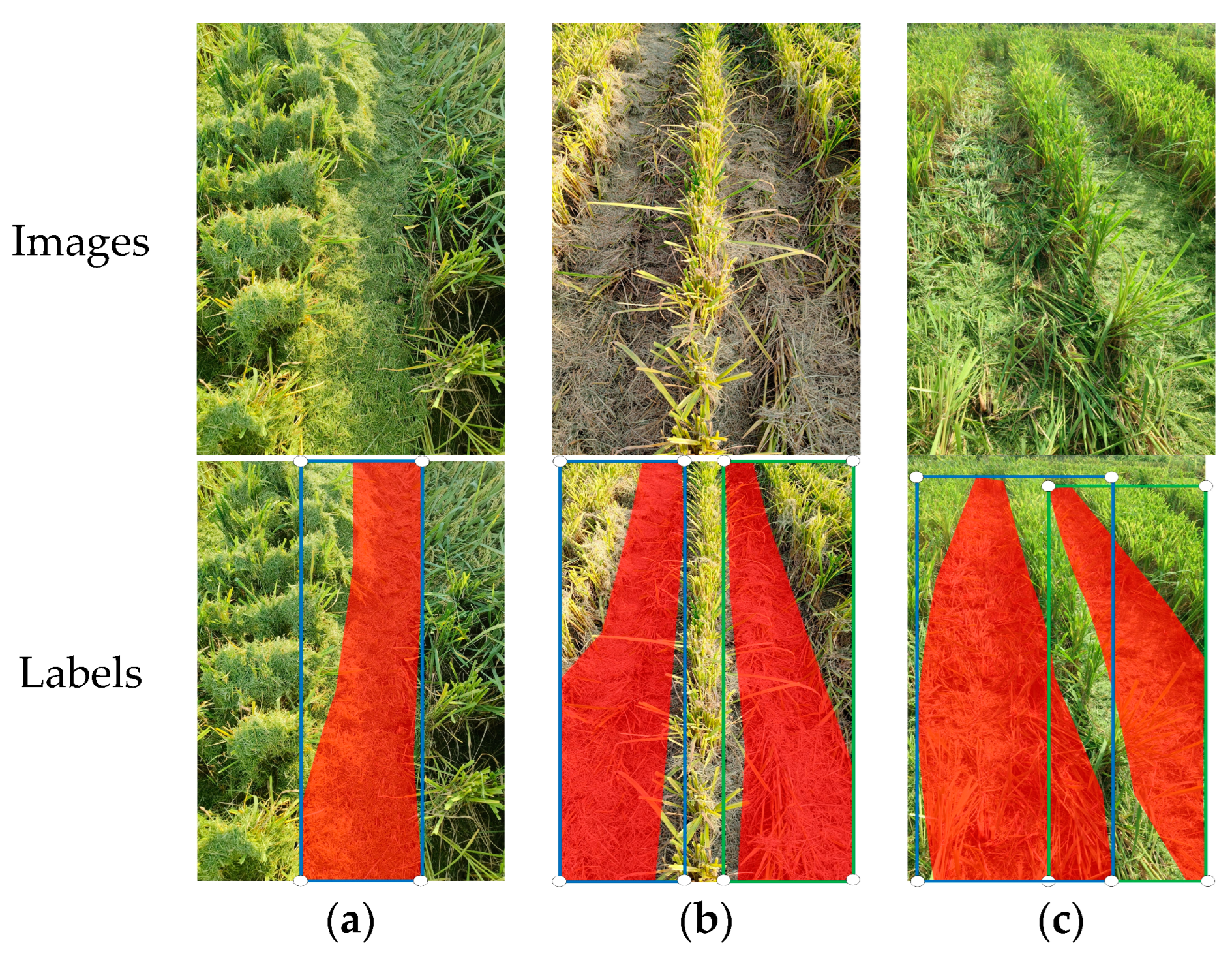
All experimental data were collected during the daytime on 9 August and 10 August 2022 in Cailing Township, Duchang County, Jiujiang City, Jiangxi Province, China, within 48 h after the first season’s harvest, in sunny weather. They were photographed with the handheld collection equipment at a height of approximately 1.5 m above the ground and with the camera facing in the direction of the extension of the rolled rice stubble rows. The collection equipment was a Canon m6 camera; 856 images were collected, each containing 1~2 complete rolled rice stubble rows. The rolled rice stubble rows in the field can be divided into three main categories:

• Heavily covered by straw discharged from the harvester.
• When just after harvesting, with a straw-green color.
• When the harvest is finished a few hours later, yellowish in color.

These three categories are displayed as shown in Figure 1.

All the collected images were cropped, and the resolution was standardized to 1080 × 1920, and LabelMe software was used to label the images. Each target object in each image is labeled with segmentation and localization information, and there is only one object category, i.e., the rolled rice stubble row, and the labeled image is shown in Figure 1. The labeled images were enhanced by randomly flipping them horizontally to double their number, and the training and test sets were divided in a ratio of 8:2 to obtain 1317 images for the training set and 397 images for the test set.

2.2. Simplified Mask R-CNN for Rolled Rice Stubble Row Segmentation

Mask R-CNN is a powerful model that not only performs object detection functions but also generates masks on the detected objects. However, this powerful capability also brings with it a high hardware resource consumption and slow prediction speed. For this reason, two successive simplifications are made based on Mask R-CNN: (i) the structure of the model is modified, and an optimization method is proposed to improve the segmentation performance of the modified model, and the theoretical basis for the model modification and optimization method is introduced in Section 2.2.1 and Section 2.2.2, respectively. (ii) The simplification of the backbone network based on the level of utilization of the feature maps by the model is presented in Section 2.2.3.

The Mask R-CNN mentioned in this paper refers to the version using ResNet-50-FPN as the backbone, which has a better performance compared to the version using ResNet-50-C4; please refer to [43,47] for details.

2.2.1. Simplification of the Second Stage of Mask R-CNN

For the segmentation task of rolled rice stubble rows, there is only one object class to be segmented, i.e., rolled rice stubble rows. If the foreground and background are used to distinguish the content in a picture, the rolled rice stubble rows that need to be segmented belong to the foreground, and those that do not need to be segmented are the background. So, the objective of the rolled rice stubble rows segmentation task can be simplified to segment the foreground from the background; based on this conclusion, a simplified scheme for Mask R-CNN was obtained based on the theoretical analysis in the following paragraph.

The structure of the Mask R-CNN is shown in Figure 2. Mask R-CNN consists of two stages; the first stage on the left consists of a backbone network and a Region Proposal Network (RPN) [48]. The function of the first stage is to perform coarse classification of targets in the image, distinguishing only between foreground and background and then generating region proposals, which are foreground regions that the model believes a target may exist. The second stage on the right consists of three branches, one for predicting the target mask and two branches for the correction and classification of the region proposals, respectively. Thus, in the first stage, Mask R-CNN can distinguish the rolled rice stubble rows from the background. Therefore, if the proposed area is sufficiently precise, it is feasible to use the region proposals as a mask generation area.

Based on the above analysis, the structure of Mask R-CNN is modified by retaining only the mask generation branch of the second stage and discarding the other two branches, and using the region proposals as the mask generation region, the specific structure after the above modification is shown in the light blue background part of the second stage in Figure 2. In this paper, we call the model with the above modifications SMR (Abbreviation of Simplified Mask R-CNN).

2.2.2. Optimization Method for SMR

Since there was no region proposals correction part in the second stage of SMR, the quality of region proposals directly determines the segmentation quality. The region proposals are usually coarse, and they do not cover the target well. In order to improve the quality of the region proposals, it is necessary to analyze the process of generating the region proposals.

The region proposals are transformed from the anchors, which are rectangular boxes distributed aimlessly over the input image. The detection process only detects the area covered by the anchors instead of traversing the whole image to improve the speed of the operation. During the prediction process, each anchor box is assigned a score, with higher scores indicating a higher probability of the presence of the target object. Then, the region proposals are transformed from the top 100 highest-scoring anchors by the following transformation formula:

$$\begin{array}{cc}x ={ t}_x w_a+x_a& w =e^{t_w} w_a\\ y ={ t}_y h_a+y_a& h =e^{t_h} h\end{array}$$

(1)

$e$ is a natural constant. $x$ and $y$, $w$ and $h$ indicate the coordinates of the center of the region proposals on the image and the width and height of the proposed region proposals. The $t_x$ denotes the amount of variation in the x-coordinate of the center of the anchors predicted by the model; $w_a$ indicate the width of the anchors; $x_a$ indicate the x-coordinate of the center of the anchors, and so on for the meaning of the other variables. From Equation (1), it is clear that the size and position of the region proposals are related to the value of the model prediction and the size and position of the anchors.

For a trained SMR model, the predicted value of the model cannot be changed, so the only way to improve the region proposals is to improve the anchors. For the five feature maps in SMR, each position on each feature map corresponds to a set of anchors, and the size and position of each set of anchors on the image is determined by the hyperparameters SCALE, RATIO, and STRIDE, In fact, the value of STRIDE has been taken to be the most optimum, for the 5-stage feature maps P2–P6, STRIDE = {4, 8, 16, 32, 64} to ensure that the generated anchors are evenly distributed over the input images, while for SCALE and RATIO, the area and aspect ratio of the anchors are controlled respectively, the effect of these three hyperparameters on the anchors is shown in part (a) of Figure 3. The key hyperparameters for improving the performance of segmentation were finally determined experimentally to be SCALE, which is described in detail in Section 3.3.

In addition, there is one detail that needs to be clarified here before the region proposals are output, they need to be subjected to NMS (Non-Maximun Suppression) [49] based on IoU to reduce the redundancy of the region proposals, and the IoU threshold is 0.5 in SMR.

2.2.3. Simplification of Backbone Network for SMR

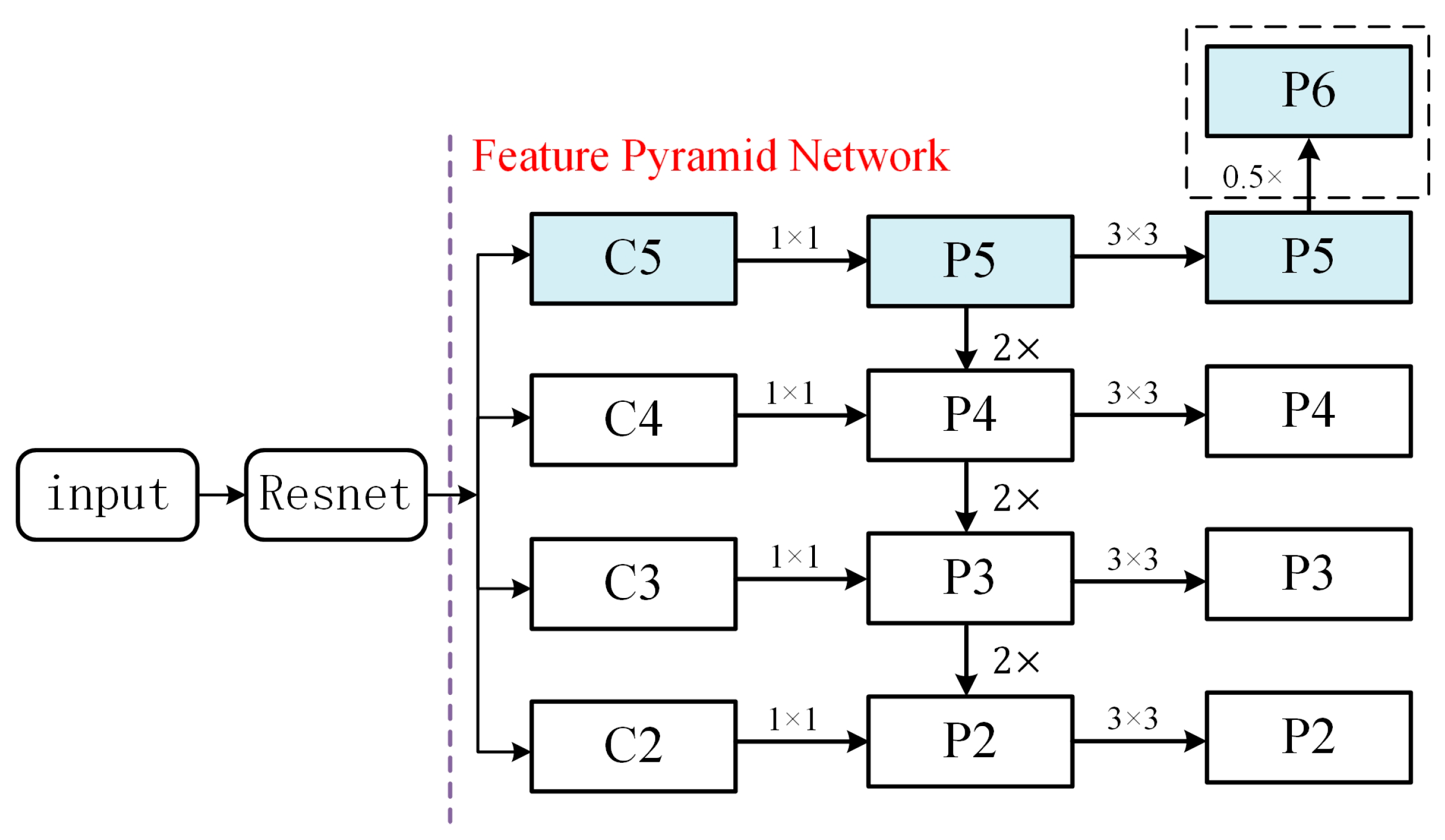
The backbone network of SMR is a combination of ResNet [50] + FPN [47], as shown in Figure 4. ResNet on the left is the feature extractor, and FPN on the right merges the features and finally outputs a 5-level feature map P2–P6. Here two sections are input into all feature maps, the RPN network and RoI Align [43], but in practice, not all feature maps need to be used for the task of segmenting the rolled rice stubble rows, and the use of feature maps in these two sections is described below.

(1)

In the RPN, all feature maps are used to generate anchors as shown in part (a) of Figure 3, but in practice, for the segmentation task of rolled stubble rows, the higher scoring region proposals are only associated with the feature maps P5 and P6 and are most related to P5, the others do not contribute in a positive way in the process of inference. (See Section 3.4 for details).

(2)

In the second stage of RoI Align, feature maps are used to generate masks. Research has shown that the larger an object is in a picture, the larger the receptive field required to recognize it [51], and for the five feature maps P2–P6 in SMR, the receptive field increases in steps, and the size decrease. Based on this, in the RoI Align, different feature maps are selected depending on the area of the RoI (Region of Interest); in SMR, the RoI is the region proposals, and the specific selection rule is as in part (b) of Figure 3. For the 1920 × 1080 resolution image used in this paper, the area of the smallest region proposals that can completely enclose the rolled rice stubble rows is typically greater than 448², corresponding to the use of feature map P5 to generate the mask. It was worth noting that feature map P6 was not presented here because the size of P6 is too small, and despite its large perceptual field, its too-small size leads to a lack of semantic information.

Based on the above analysis, combined with the need for training, i.e., in order to avoid the use of a single feature map resulting in insufficient samples, which in turn leads to slow loss convergence, feature maps P5 and P6 are used in training and P6 is removed in inference. The simplified structure is shown in Figure 4. The light blue background part is the structure retained after the simplification (the structure in the dashed box will be removed when using only feature map P5), and the simplified backbone network only retains the parts associated with feature maps P5 and P6. The rules for feature map selection remain the same as in Figure 3.

So far, all the simplifications have been completed, and the SMR after the backbone network simplification is called SMR-RS (abbreviation of simplified Mask R-CNN for rolled rice stubble row segmentation), and its intuitive comparison with Mask R-CNN is shown in Figure 2.

2.3. Loss

Compared to Mask R-CNN, SMR, and SMR-RS do not need to calculate the loss of classification and the loss of bbox (bounding box) regression in the second stage, and only two categories need to be calculated in classification loss; its losses are as follows:

$${loss}_{rpn\_cls}=-\left(y_a\log \left(x_a\right)+\left(1 -y_a\right)\log \left({1 -x}_a\right)\right)$$

(2)

$${loss}_{rpn\_bbx}=\left\{\begin{array}{c}\begin{array}{cc}0.5{\left({ t}_y-t_x\right)}^2& \mathrm{if}\left|{ t}_y-t_x\right|<1\end{array}\\ \begin{array}{cc}\left|{ t}_y-t_x\right|& \mathrm{otherwise}\end{array}\end{array}\right.$$

(3)

$${loss}_{mask}=-\frac{1}{N}\sum _{i=1}^N\left(y_m^i\log \left(x_m^i\right)+\left(1-y_m^i\right)\log \left(1 -x_m^i\right)\right)$$

(4)

$$loss={loss}_{rpn\_cls}+{loss}_{rpn\_bbx}+{loss}_{mask}$$

(5)

where ${loss}_{rpn\_cls}$ denotes the classification loss in the RPN, ${loss}_{rpn\_bbx}$ denotes the bbox regression loss in the RPN, ${loss}_{mask}$ denotes mask loss in the second stage. $y_a$ represents the target value of the anchor category, $x_a$ represents the predicted value of the anchor frame category, $t_y$ represents the target value of the anchor size and position parameters, $t_x$ represents the predicted value of the anchor size and position parameters, $N$ represents the number of pixels for category prediction, $y_m^i$ represents the target value of the ith pixel category, and $x_m^i$ represents the predicted value of the ith pixel category. Other unmentioned details of loss calculation are consistent with Mask R-CNN.

3. Results and Analysis

3.1. Platform Parameters and Training

In this study, the model was trained using a server with a Xeon(R) Platinum 8358P CPU and NVIDIA^® V100 32G GPU. The key hyperparameters used in the training process are shown in

Table 1. Key hyperparameters of training.

Hyperparameters	Value
Optimizer	SGD
Momentum	0.90
Weight decay	1.00 × 10−4
Initial learning rate	2.00 × 10−5
Max epoch	100
Minibatch size	8
Learning rate scheduler	Warmup + MultiStep drop
Warmup period	0–500 iters
Learning rate after Warmup	0.02
Learning rate drop steps	40th, 60th epoch
Learning rate drop factor	0.10

, and the loss of the training process is shown in Figure 5; it can be observed that the loss of SMR and SMR-RS is lower than that of Mask R-CNN, and SMR is particularly significant.

The model test was running on a local PC with an AMD Ryzen 7 5800 H 3.20 GHz CPU and an NVIDIA GeForce RTX 3070 Laptop GPU. The programming language used for both training and testing is Python, and the deep learning framework used is Pytorch.

3.2. Evaluation Index

This paper uses intersection over union (IoU), harmonic average (F1), total number of model parameters, GPU memory occupancy when predicting, and average run time per image to evaluate the performance of the trained model. The corresponding formulas are as follows:

$$\mathit{Precision}=\frac{TP}{TP+FP}$$

(6)

$$\mathit{Recall}=\frac{TP}{TP+FN}$$

(7)

$$IoU=\frac{TP}{TP+FN+FP}$$

(8)

$$F1=\frac{2\mathit{Precision}\ast \mathit{Recall}}{\mathit{Precision} + \mathit{Recall}}$$

(9)

where $TP$ indicates that the model prediction and label values are both positive, $FP$ indicates that the prediction is true and the label value is false, and $FN$ indicates that the prediction is false and the label value is positive. $IoU$ is a common evaluation metric used in this paper to indicate the degree of overlap between the mask predicted by the model and the label mask. The $F1$ value is the harmonic mean of precision and recall, which is equivalent to the combined evaluation metric of precision and recall. The values of the evaluation obtained below are averaged over all the images in the test set.

3.3. Optimization Experiments for SMR

The segmentation performance of the original SMR on the test set is shown in

Table 2. SMR performance before and after optimization.

Method	IoU	F1	Parameters/M	Memory/Mb	t/ms
Mask R-CNN	0.826	0.906	43.7	862.0	132.0
SMR	0.126	0.217	29.8	808.0	123.8
SMR-40	0.829	0.909	29.8	808.0	123.8

. Compared with Mask R-CNN, the number of parameters of SMR was reduced significantly, from 43.7 M to 29.8 M, a reduction of 31.8%, and the GPU memory consumption was reduced by 6.3% prediction speed was increased by 6.2%, the training loss is slightly smaller, as in Figure 5, but the segmentation mask quality was significantly reduced. To solve this problem, SMR was optimized for experiments, and the segmentation performance of SMR after optimization even surpassed that of Mask R-CNN, and this optimization trial process is described below.

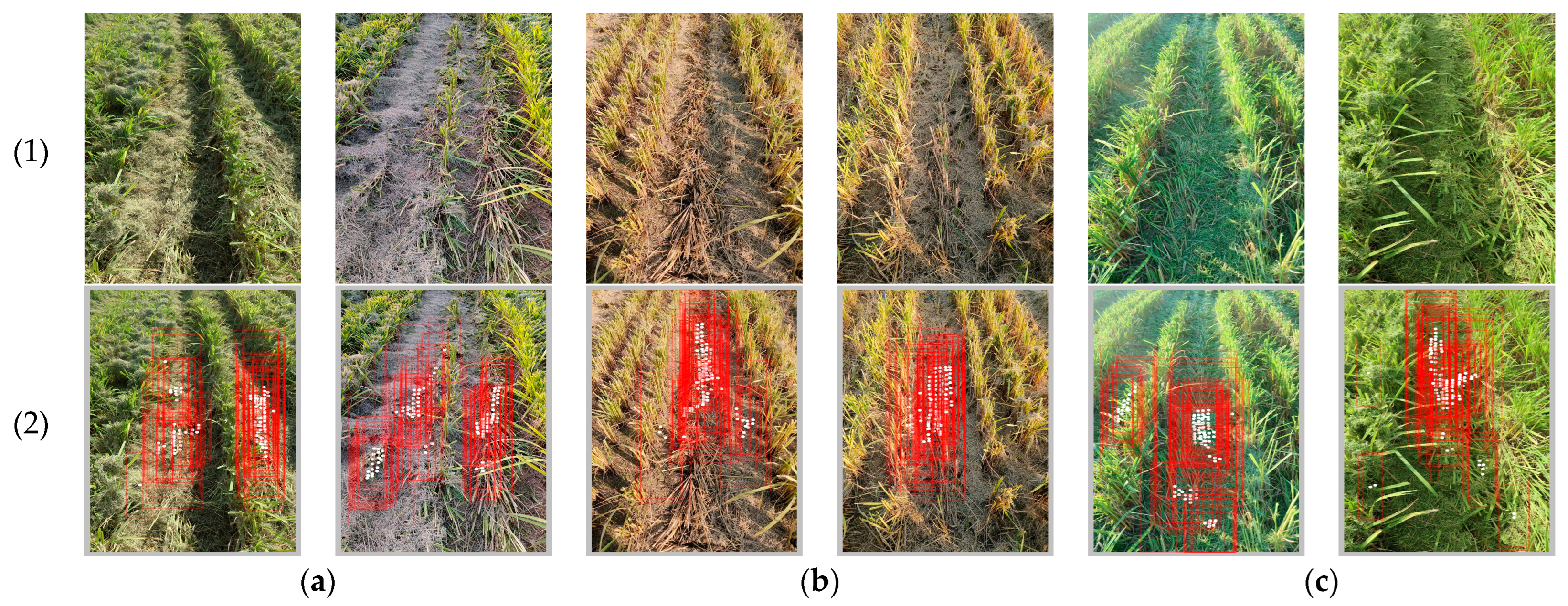
To explain the specific reasons for the poor segmentation performance of the original SMR, the prediction results of the region proposals in the test set are shown in Figure 6; each of these images shows the top 100 region proposals (before NMS). It is clear that although the region proposals were above the row of rolled rice stubble, it is so small that it only covered a small part of the row.

According to Section 2.2.2, the size of the region proposals can be changed by modifying the hyperparameters SCALE and RATIO. In the original SMR, the values of SCALE and RATIO are consistent with Mask R-CNN, which are SCALE = 8 and RATIO = {0.5, 1, 2} [47]. On this basis, the SCALE value of SMR was made to increase from 8 to 16, 24, 32, 40, and 48 at the same time as RATIO varies by a factor of 0.2, 1, and 5 during the process of inference. The IoU performance of SMR and Mask R-CNN under simultaneous changes of SCALE and RATIO is shown in Figure 7.

From Figure 7 for the Mask R-CNN, changes in SCALE and RATIO barely improve IoU performance and bring it down. However, for SMR, as the value of SCALE increased from 8 to 32, the IoU gradually increased and continued to increase from 32 to 48; the IoU did not increase significantly. In contrast, the change in the value of RATIO has a less strong effect on the IoU, but there was still a certain pattern to follow, with all SCALE conditions having higher values of IoU at 1.0×, i.e., at the original RATIO. The performance of the mask at SCALE = 40 and RATIO = {0.5, 1, 2} is shown in Table 2 in row SMR-40, which indicates that the quality of the mask exceeds that of Mask R-CNN. According to the above experimental results, the reason for the poor quality of the original SMR segmentation mask is that the SCALE is too small, and using a larger value for prediction can effectively improve the quality of the mask; changing the RATIO to deviate from the original would cause to a decrease.

In order to investigate the performance of SMR under different values of SCALE of training, the SMR was trained using SCALE = 16 and 24, respectively (the reason for not continuing to increase the SCALE value is that the model converges slowly in the training process after further increase), and then adjusting the SCALE value in the prediction process to optimize the mask quality. The results are shown in

Table 3. Performance of SMR under training at different SCALE.

SCALE		IoU	F1	Parameters/M	Memory/Mb	t/ms
Train	Predict
16	16	0.648	0.790	29.8	808.0	123.8
16	24	0.803	0.896	-	-	-
16	30	0.828	0.909	-	-	-
24	24	0.782	0.890	29.8	808.0	123.8
24	30	0.819	0.904	-	-	-
24	48	0.830	0.910	-	-	-

, which indicates that increasing the value of SCALE in the training process can improve the initial mask quality, but the optimal mask quality still needs to be achieved by adjusting the SCALE in the prediction process, and there is no significant relationship between the optimal mask quality and the SCALE value in the training process.

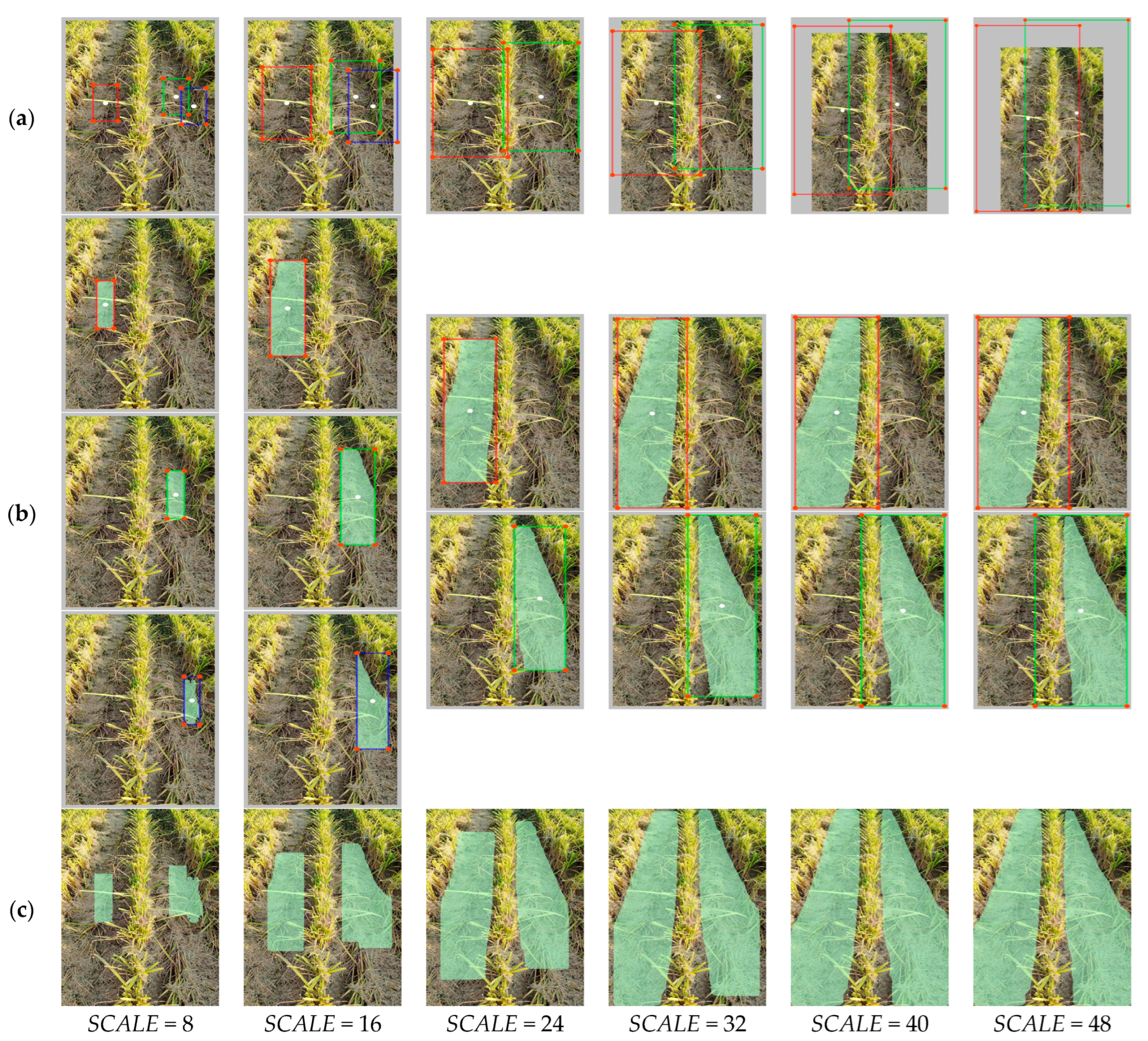
In order to visually explain the mechanism of the effect of variation in SCALE on the prediction mask, the anchors, region proposals, and masks of the SMR in the prediction process under different SCALE values were tracked, and one of the representative results was selected as shown in Figure 8. For SCALE = 8, 16, 24, 32, and 40, the model found the exact location of the stubble rows and presented at least one regional proposal centered on each of the rows, the difference being that for SCALE = 8, the anchor size was small and the resulting region proposals were similarly small, covering only a small portion of the rolled stubble rows and therefore only a small portion of the mask. As the SCALE increases, the size of the anchors increases, and so does the size of the region proposals. For the region proposals with the center point on the stubble row, the larger the size means that the complete stubble row is covered, and therefore the mask generated in the region proposals is more complete; at SCALE = 32, the mask was able to cover almost the complete rolled rice row. As SCALE continued to increase to 40 and 48, the anchors continued to increase, while the region proposals did not change significantly; in turn, the mask changes were not obvious.

The reason why the size of the region proposals increased as the anchor increased is that, according to

Table A1. Formula of calculating the height (H) and width (W) of the anchors when SCALE = x, STRIDE = {m, n,⋯}, RATIO = {a, b,⋯}. (Derived from source code provided by the authors of the paper [43].)

STRIDE	RATIO = a	RATIO = b	• • • *
m	H = mx√a, W = mx/√a	H = mx√b, W = mx/√b	• • •
n	H = nx√a, W = nx/√a	H = nx√b, W = nx/√b	• • •
• • •	• • •	• • •	• • •

* Expresses omission.

, as SCALE increased, the size of the anchors increased, and from Equation (1), the larger the size of the anchors, the larger the size of the region proposals, and as SCALE increases from 32 to 40 and 48 in Figure 8, the size of the region proposals does not change significantly because the region proposals that are outside the scope of the image will be cropped out.

3.4. SMR Backbone Network Simplification Experiment

The performance of SMR-RS is shown in

Table 4. Comparison of the performance of the SMR-RS and the SMR-40.

Model	IoU	F1	Parameters/M	Memory/Mb	t/ms
SMR-40	0.829	0.909	29.8	808.0	123.8
SMR-RS	0.843	0.915	27.6	549.0	77.4

, compared to SMR-40, which was obtained after optimizing SMR, the total parameters are reduced by 7.4%, the prediction speed is increased by 37.5%, the GPU occupation is reduced by 32.1%, the IoU value is increased by 1.5%, and the F1 value is increased by 0.6%. To achieve these, statistics are presented in the following paragraphs on the utilization of feature maps by SMR as a basis for targeted censoring of the backbone network.

In the process of predicting the test set using SMR, it was found that most of the anchors with high scores had relatively similar sizes. Since the size of anchors generated by the same feature map is the same, it is guessed that most of the high-scoring anchors may come from the same feature map, and the feature map attribution of the anchors can be inferred from Table A1 based on the size of the anchors. For example, it is known that the H × W of the area of one of the highest scoring anchors is 4096, and the hyperparameter SCALE is 8, the STRIDE is known to be 8 from Table A1, and the anchor belongs to the feature map P3 according to the correspondence between the STRIDE and the feature map. Based on this, the sizes of anchors with the top 100 scores predicted by SMR (trained at three different SCALE) on the test set were counted, and the feature map attribution of anchors was also calculated, and the results are shown in

Table 5. Statistical results of feature map attribution for anchors.

Method	P2	P3	P4	P5	P6
SCALE-8	0	0	0	86%	14%
SCALE-16	0	0	0	72%	28%
SCALE-24	0	0	0	80%	20%

.

From

Table 6. Results of the SMR backbone network simplification experiment.

Method	IoU	F1	Parameters/M	Memory/Mb	t/ms
SMR-40	0.829	0.909	29.8	808.0	123.8
P5-P6	0.836	0.912	27.6	549.0	79.2
P5	0.843	0.915	27.6	549.0	77.4
P6	0.702	0.832	27.6	549.0	77.1

, it is clear that these anchors accounted for the vast majority on P5, a small percentage on P6, and 0 on P2, P3, and P4, so it can be assumed that feature maps P2, P3, and P4 did not contribute positively to the prediction results. To explore the effect of feature maps P5 and P6 on inference results, the SMR of the simplified backbone network was trained, and the trained model was tested under the following methods with SCALE taken as 40:

• Using feature maps P5 and P6.
• Using feature map P5 only.
• Using feature map P6 only.

Their performance on the test set is shown in Table 6, where it can be seen that the segmentation performance is better in methods 1 and 2, with no degradation compared to the SMR-40, and was slightly improved in method 2 and underperformed in method 3.

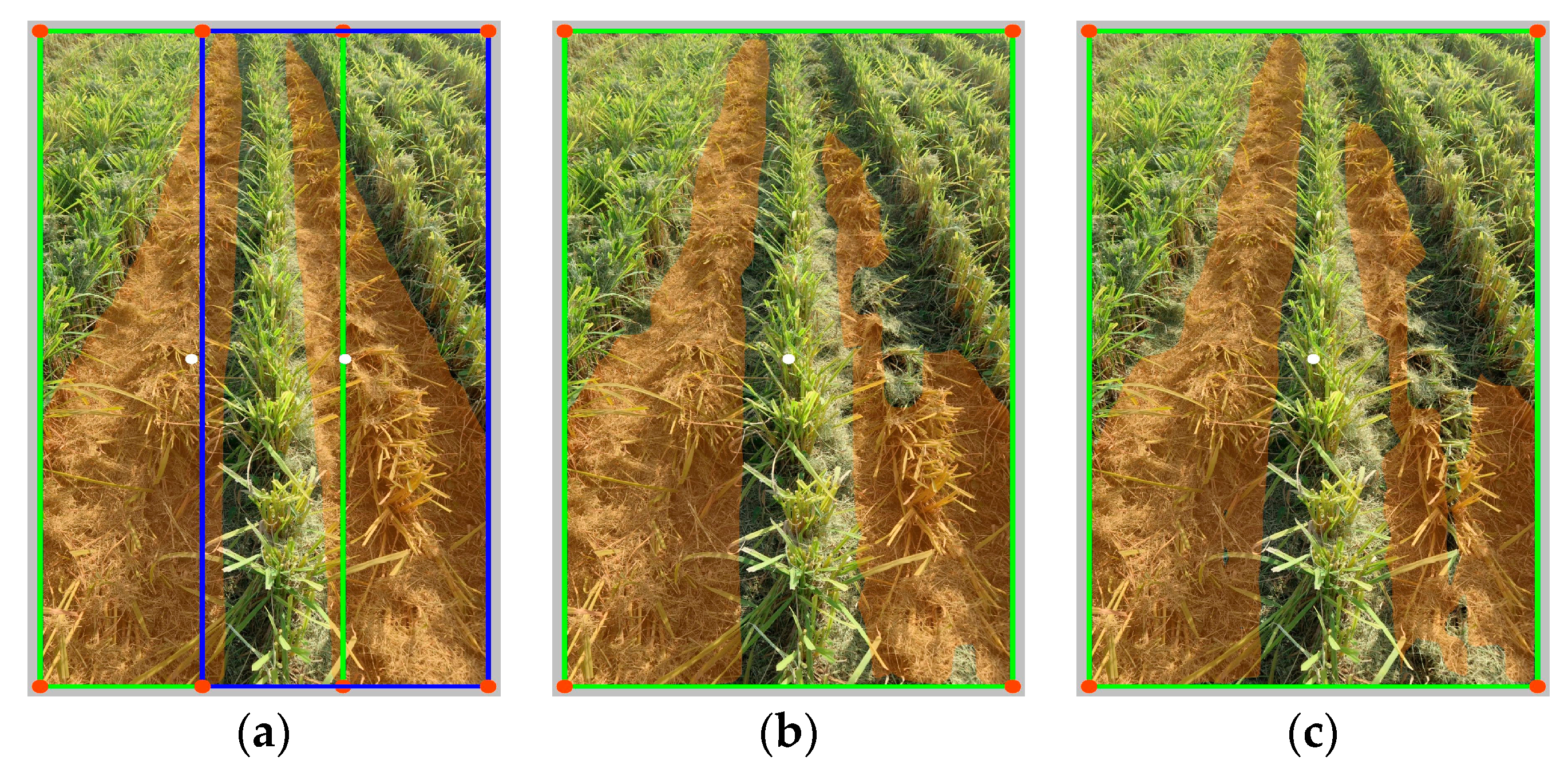
As shown in Figure 9, both method 1 and method 3 perform less well than method 2 in terms of segmentation due to the influence of the feature map P6, which generated lower quality region proposal. Although the region proposal was identical for methods 1 and 3, the lack of semantic information in feature map P6 in method 3 caused a reduction in the quality of the mask.

3.5. Time Consumption Analysis

In order to investigate how the above-simplified operation can reduce the running time, the SMR, SMR-RS, and Mask R-CNN are divided into three parts: backbone network, RPN, and second stage. The average prediction elapsed time calculated on the test set is shown in

Table 7. Three parts of time consumption statistics (ms).

Model	Backbone	RPN	Second Stage	Total
Mask R-CNN	6.7	114.0	11.3	132.0
SMR	6.7	114.0	3.1	123.8
SMR-RS	6.1	68.2	3.1	77.4

; compared with Mask R-CNN, the time of the second stage was reduced by 72.5%, while the other parts were unchanged. On the whole, the main time consumption part of Mask R-CNN is the RPN, which accounts for 86.4% of the total time consumed, while the second stage accounts for only 8.6%, which resulted in a small improvement in the overall prediction speed of SMR compared to Mask R-CNN. The significant reduction in the time consumed by SMR-RS compared to SMR was due to the significant reduction in time consumed by the RPN.

3.6. Comparison of the Performance of Different Models

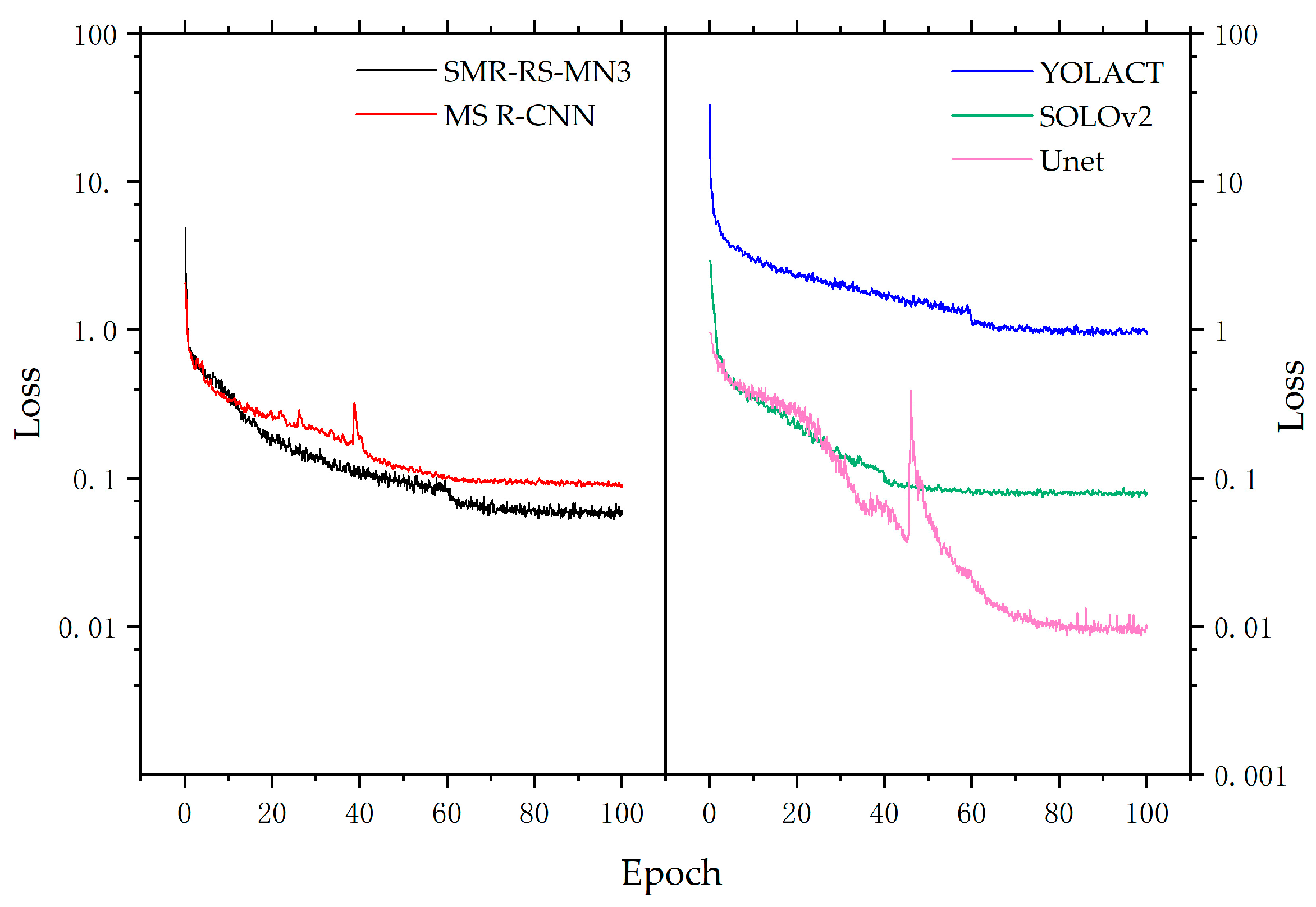
The instance segmentation models SOLOv2 [52] and Mask Scoring R-CNN [53], YOLACT [54], SMR-RS with MobileNetv3-Large [55] as the backbone network feature extractor (SMR-RS-MN3) and semantic segmentation model Unet [32] were trained according to the parameter settings in Table 1, training losses are shown in Figure 10, and the results obtained for each model on the test set are shown in

Table 8. Performance of seven models.

Model	IoU	F1	Parameters/M	Memory/Mb	Flops 1	t/ms
SMR-RS	0.843	0.915	27.6	549.0	1.76 × 1012	77.4
SMR-RS-MN3	0.834	0.910	6.7	338.0	1.32 × 1012	23.5
Mask R-CNN	0.826	0.906	43.7	862.0	4.08 × 1012	132.0
SOLOv2	0.839	0.915	46.2	893.0	4.26 × 1012	150.0
Mask SR	0.827	0.907	44.1	932.0	4.08 × 1012	139.9
YOLACT	0.829	0.909	35.3	581.0	4.02 × 1012	127.8
Unet 2	0.790	0.885	29.0	2491.0	8.09 × 1012	13.9

¹ The number of floating-point operations required to infer a single image was calculated using a Python library called thop. ² The input image is cropped to 1024 × 1024 to meet the model’s requirements for resolution.

. SMR-RS slightly outperforms SOLOv2, YOLACT, and Mask Scoring R-CNN in terms of segmentation performance and has a significant advantage in terms of total parameters, GPU memory occupation, Flops, and running speed, outperforming SOLOv2 by 40.3%, 38.5%, 58.7% and 48.4%, YOLACT by 21.8%, 5.5%, 56.2% and 39.4% and Mask Scoring R-CNN by 37.4%, 41.1%, 56.9%, and 44.0%. Due to its lightweight backbone, the SMR-RS-MN3 has a further reduction in running time consumption and hardware resource consumption from the SMR-RS. However, this also resulted in a reduction in the quality of the segmentation. The performance of the SMR-RS-MN3 demonstrates the scalability of the SMR-RS. Although Unet has a significant inference speed advantage at lower resolutions, it has higher hardware requirements, consumes far more GPU memory and computational power (Flops), and is inferior to other models in segmentation accuracy.

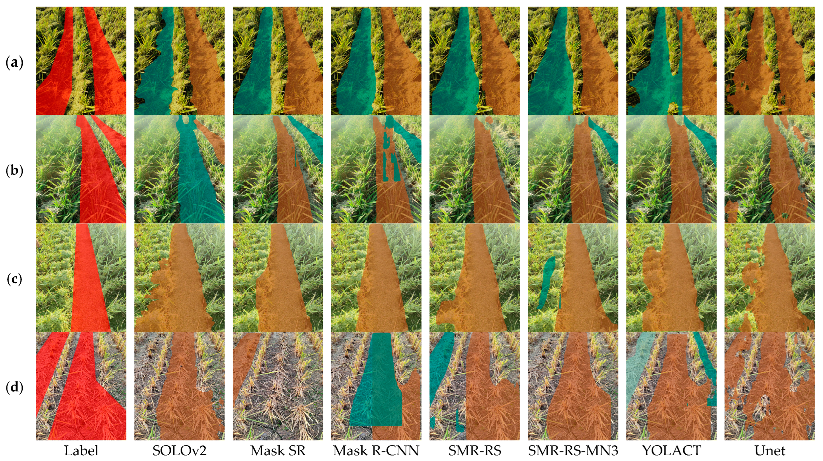
As shown in Figure 11, the mask prediction results of the proposed model in this paper are compared with those of the state-of-the-art model; there are four representative images, as shown in (a), (b), (c), and (d). As shown in (d), for these two complexes rolled rice stubble rows, only SMR-RS and YOLACT identified all of them, but YOLOCT misidentified a non-rice stubble row, and as shown in (b); SMR-RS was insensitive to a small area of rice stubble rows. For these four images, SMR-RS-MN3 performed well overall, but for the stubble rows that were heavily straw-covered in (c), it identified a small area of unrolled rice stubble rows as rolled rice stubble rows; SOLOv2 also performed well, but the edge segmentation of rolled rice stubble rows is poor, as shown in (a), (c); Mask Scoring R-CNN has a serious under-recognition phenomenon, and the large area of rice stubble rows located in the center of (d) is not recognized; Mask R-CNNN has the phenomenon of repeated recognition, as shown in (b), (d); Unet only achieves semantic segmentation, and there are multiple small regions of false segmentation in these results.

4. Conclusions

(1)

This paper presented a novel approach to improving a model without adding to or replacing any existing advanced modules on the original model. The model was improved by analyzing the effects of the individual components of the model. Firstly, based on the functions of the first stage and second stage, two of the three functional branches in the second stage of Mask R-CNN are removed, and only the mask generation branch is retained, and the region proposals output from the first stage was directly used as the mask generation region to obtain a preliminary simplified model SMR. The key parameter affecting its segmentation quality was obtained through theoretical analysis and experiments, and its segmentation performance was greatly improved by simple adjustment of this parameter. Further, a theoretical and experimental analysis of the extent to which the SMR utilized the feature map in the task of segmenting rolled rice stubble rows was carried out as a basis for simplifying the backbone network to obtain SMR-RS.

(2)

SMR-RS can be seen as a single-stage model with a mask generation module attached but still implements instance segmentation. Compared to Mask R-CNN, SMR-RS ran 41.4% faster, with a single image processing time of only 77.4 ms, meeting the real-time requirements of fieldwork; 36.8% fewer parameters and 36.3% less GPU memory occupation, making it more suitable for deployment on mobile devices; the IoU value of SMR-RS reaches 0.843, and the F1 value was 0.915. Compared to other advanced instance segmentation models, SMR-RS also achieved a significant reduction in prediction time consumption and hardware resource usage with slightly better segmentation results. The model improvement methods in this paper can provide a reference for other researchers, and the proposed instance segmentation model can provide technical support for the implementation of automatic row alignment for stubble-lifting machines.

In addition, SMR-RS is also highly extensible, and the model’s performance was further improved by using more advanced modules, which is one of the directions for future research.

References

1. Firouzi, S.; Nikkhah, A.; Aminpanah, H. Rice Single Cropping or Ratooning Agro-System: Which One Is More Environment-Friendly? Environ. Sci. Pollut. Res. 2018, 25, 32246–32256. [Google Scholar] [CrossRef] [PubMed]
2. Fang, W.; Li, L.; Dai, S. Tehniques of Ratoon Rice in Northern Zhejiang Province and Its Benefit. China Rice 2019, 25, 132–134. [Google Scholar]
3. Harrell, D.L.; Bond, J.A.; Blanche, S. Evaluation of Main-Crop Stubble Height on Ratoon Rice Growth and Development. Field Crops Res. 2009, 114, 396–403. [Google Scholar] [CrossRef]
4. Pasaribu, P.O.; Triadiati; Anas, I. Rice Ratooning Using the Salibu System and the System of Rice Intensification Method Influenced by Physiological Traits. Pertanika J. Trop. Agric. Sci. 2018, 41, 637–654. [Google Scholar]
5. Dong, H.; Chen, C.; Wang, W.; Peng, S.; Hang, J.; Cui, K.; Nie, L. The growth and yield of a wet-seeded rice-ratoon rice system incentral China. Field Crops Res. 2017, 208, 55–59. [Google Scholar] [CrossRef]
6. Liu, J. Design and Test of Righting for Rolled Ratooning Rice Stubbles in First Harvest. Master’s Thesis, Jiangsu University, Zhenjiang, China, 2022. [Google Scholar]
7. Xiao, S. Effect of Mechanical Harvesting of Main Crop on the Grain Yield and Quality of Ratoon Crop in Ratooned Rice. Master’s Thesis, Hua Zhong Agriculture University, Wuhan, China, 2018. [Google Scholar]
8. Chen, X.; Li, H.; Liu, M.; Yu, J.; Zhang, X.; Liu, Z.; Peng, Y. Stubble Righting Increases the Grain Yield of Ratooning Rice After the Mechanical Harvest of Primary Rice. J. Plant Growth Regul. 2022, 41, 1747–1757. [Google Scholar] [CrossRef]
9. Zhang, X. Design and Experiment of Regenerative Rice Chain Row Claw Type Righting Device. Master’s Thesis, Jiangxi Agriculture University, Nanchang, China, 2019. [Google Scholar]
10. Chen, X.; Liang, X.; Liu, M.; Yu, J.; Li, H.; Liu, Z. Design and experiment of finger-chain grain lifter for ratoon rice stubble rolled by mechanical harvesting. Inmateh Agric. Eng. 2022, 1, 361–372. [Google Scholar] [CrossRef]
11. Grau, V.; Mewes, A.U.J.; Kikinis, R.; Warfield, S.K.; Alcañiz, M. Improved Watershed Transform for Medical Image Segmentation Using Prior Information. IEEE Trans. Med. Imaging 2004, 23, 447–458. [Google Scholar] [CrossRef]
12. Qin, A.K.; Clausi, D.A. Multivariate Image Segmentation Using Semantic Region Growing with Adaptive Edge Penalty. IEEE Trans. Image Process. 2010, 19, 2157–2170. [Google Scholar] [CrossRef]
13. Chen, Y.; Weng, G. An Active Contour Model Based on Local Pre-Piecewise Fitting Image. Optik 2021, 248, 168130. [Google Scholar] [CrossRef]
14. Chen, Y.; Ge, P.; Wang, G.; Weng, G.; Chen, H. An Overview of Intelligent Image Segmentation Using Active Contour Models. Intell. Robot. 2023, 3, 23–55. [Google Scholar] [CrossRef]
15. Yu, Y.K.; Wong, K.H.; Chang, M.M.Y. Pose Estimation for Augmented Reality Applications Using Genetic Algorithm. IEEE Trans. Syst. Man Cybern. Part B 2005, 35, 1295–1301. [Google Scholar] [CrossRef] [PubMed]
16. O’Mahony, N.; Campbell, S.; Carvalho, A.; Harapanahalli, S.; Hernandez, G.V.; Krpalkova, L.; Riordan, D.; Walsh, J. Deep Learning vs. Traditional Computer Vision. In Advances in Computer Vision; Arai, K., Kapoor, S., Eds.; Springer International Publishing: Cham, Switzerland, 2020; pp. 128–144. [Google Scholar]
17. Rabab, S.; Badenhorst, P.; Chen, Y.-P.P.; Daetwyler, H.D. A Template-Free Machine Vision-Based Crop Row Detection Algorithm. Precis. Agric. 2021, 22, 124–153. [Google Scholar] [CrossRef]
18. Bah, M.D.; Hafiane, A.; Canals, R. Hierarchical Graph Representation for Unsupervised Crop Row Detection in Images. Expert Syst. Appl. 2023, 216, 119478. [Google Scholar] [CrossRef]
19. Ma, Z.; Tao, Z.; Du, X.; Yu, Y.; Wu, C. Automatic Detection of Crop Root Rows in Paddy Fields Based on Straight-Line Clustering Algorithm and Supervised Learning Method. Biosyst. Eng. 2021, 211, 63–76. [Google Scholar] [CrossRef]
20. Zhang, T.; Xia, J.F.; Wu, G.; Zhai, J.B. Automatic navigation path detection method for tillage machines working on high crop stubble fields based on machine vision. Int. J. Agric. Biol. Eng. 2014, 7, 29–37. [Google Scholar]
21. Yang, Y.; Zhou, Y.; Yue, X.; Zhang, G.; Wen, X.; Ma, B.; Xu, L.; Chen, L. Real-Time Detection of Crop Rows in Maize Fields Based on Autonomous Extraction of ROI. Expert Syst. Appl. 2023, 213, 118826. [Google Scholar] [CrossRef]
22. Gai, J.; Xiang, L.; Tang, L. Using a Depth Camera for Crop Row Detection and Mapping for Under-Canopy Navigation of Agricultural Robotic Vehicle. Comput. Electron. Agric. 2021, 188, 106301. [Google Scholar] [CrossRef]
23. Liang, X.; Chen, B.; Wei, C.; Zhang, X. Inter-Row Navigation Line Detection for Cotton with Broken Rows. Plant Methods 2022, 18, 90. [Google Scholar] [CrossRef]
24. Han, C.; Zheng, K.; Zhao, X.; Zheng, S.; Fu, H.; Zhai, C. Design and Experiment of Row Identification and Row-oriented Spray Control System for Field Cabbage Crops. Trans. Chin. Soc. Agric. Mach. 2022, 53, 89–101. [Google Scholar]
25. Wang, A.; Zhang, M.; Liu, Q.; Wang, L.; Wei, X. Seedling crop row extraction method based on regional growth and mean shift clustering. Trans. Chin. Soc. Agric. Eng. 2021, 37, 202–210. [Google Scholar]
26. Gong, J.; Sun, K.; Zhang, Y.; Lan, Y. Extracting navigation line for rhizome location using gradient descent and corner detection. Trans. Chin. Soc. Agric. Eng. 2022, 38, 177–183. [Google Scholar]
27. Li, X.; Su, J.; Yue, Z.; Wang, S.; Zhou, H. Extracting navigation line to detect the maize seedling line using median-point Hough transform. Trans. Chin. Soc. Agric. Eng. 2022, 38, 167–174. [Google Scholar]
28. Wang, C.; Lu, C.; Li, H.; He, J.; Wang, Q.; Jiang, S. Image segmentation of maize stubble row based on SVM. Trans. Chin. Soc. Agric. Eng. 2021, 37, 117–126. [Google Scholar]
29. Ota, K.; Kasahara, J.; Yamashita, A.; Asama, H. Weed and Crop Detection by Combining Crop Row Detection and K-Means Clustering in Weed Infested Agricultural Fields. In Proceedings of the 2022 IEEE/SICE International Symposium on System Integration (SII), Narvik, Norway, 9–12 January 2022; pp. 985–990. [Google Scholar]
30. Li, J.; Qiao, Y.; Liu, S.; Zhang, J.; Yang, Z.; Wang, M. An Improved YOLOv5-Based Vegetable Disease Detection Method. Comput. Electron. Agric. 2022, 202, 107345. [Google Scholar] [CrossRef]
31. Sanaeifar, A.; Guindo, M.L.; Bakhshipour, A.; Fazayeli, H.; Li, X.; Yang, C. Advancing Precision Agriculture: The Potential of Deep Learning for Cereal Plant Head Detection. Comput. Electron. Agric. 2023, 209, 107875. [Google Scholar] [CrossRef]
32. Rai, N.; Zhang, Y.; Ram, B.G.; Schumacher, L.; Yellavajjala, R.K.; Bajwa, S.; Sun, X. Applications of Deep Learning in Precision Weed Management: A Review. Comput. Electron. Agric. 2023, 206, 107698. [Google Scholar] [CrossRef]
33. Cerrato, S.; Mazzia, V.; Salvetti, F.; Chiaberge, M. A Deep Learning Driven Algorithmic Pipeline for Autonomous Navigation in Row-Based Crops. arXiv 2021, arXiv:2112.03816. [Google Scholar]
34. Lai, H.; Zhang, Y.; Zhang, B.; Yin, Y.; Liu, Y.; Dong, Y. Design and experiment of the visual navigation system for a maize weeding robot. Trans. Chin. Soc. Agric. Eng. 2023, 39, 18–27. [Google Scholar]
35. Yang, Y.; Li, J.; Nie, J.; Yang, S.; Tang, J. Cotton Stubble Detection Based on Improved YOLOv3. Agronomy 2023, 13, 1271. [Google Scholar] [CrossRef]
36. De Silva, R.; Cielniak, G.; Gao, J. Towards Agricultural Autonomy: Crop Row Detection under Varying Field Conditions Using Deep Learning. arXiv 2021, arXiv:2109.08247. [Google Scholar]
37. Cao, M.; Tang, F.; Ji, P.; Ma, F. Improved Real-Time Semantic Segmentation Network Model for Crop Vision Navigation Line Detection. Front. Plant Sci. 2022, 13, 898131. [Google Scholar] [CrossRef] [PubMed]
38. Ronneberger, O.; Fischer, P.; Brox, T. U-Net: Convolutional Networks for Biomedical Image Segmentation. In Medical Image Computing and Computer-Assisted Intervention (MICCAI); Lecture Notes in Computer Science; Springer: Cham, Switzerland, 2015; Volume 9351, pp. 234–241. [Google Scholar]
39. Paszke, A.; Chaurasia, A.; Kim, S.; Culurciello, E. ENet: A Deep Neural Network Architecture for Real-Time Semantic Segmentation. arXiv 2016, arXiv:1606.02147. [Google Scholar]
40. Doha, R.; Al Hasan, M.; Anwar, S.; Rajendran, V. Deep Learning Based Crop Row Detection with Online Domain Adaptation. In Proceedings of the 27th ACM SIGKDD Conference on Knowledge Discovery & Data Mining; KDD ′21, Singapore, 14–18 August 2021; Association for Computing Machinery: New York, NY, USA, 2021; pp. 2773–2781. [Google Scholar] [CrossRef]
41. Song, Y.; Xu, F.; Yao, Q.; Liu, J.; Yang, S. Navigation Algorithm Based on Semantic Segmentation in Wheat Fields Using an RGB-D Camera. Inf. Process. Agric. 2022. [Google Scholar] [CrossRef]
42. Dos Santos Ferreira, A.; Junior, J.M.; Pistori, H.; Melgani, F.; Gonçalves, W.N. Unsupervised Domain Adaptation Using Transformers for Sugarcane Rows and Gaps Detection. Comput. Electron. Agric. 2022, 203, 107480. [Google Scholar] [CrossRef]
43. He, K.; Gkioxari, G.; Dollár, P.; Girshick, R. Mask R-CNN. In Proceedings of the 2017 IEEE International Conference on Computer Vision (ICCV), Venice, Italy, 22–29 October 2017; pp. 2980–2988. [Google Scholar] [CrossRef]
44. Long, J.; Zhao, C.; Lin, S.; Guo, W.; Wen, C.; Zhang, Y. Segmentation method of the tomato fruits with different maturities under greenhouse environment based on improved Mask R-CNN. Trans. Chin. Soc. Agric. Eng. 2021, 37, 100–108. [Google Scholar]
45. Rong, M.; Wang, Z.; Ban, B.; Guo, X. Pest Identification and Counting of Yellow Plate in Field Based on Improved Mask R-CNN. Discret. Dyn. Nat. Soc. 2022, 2022, 1913577. [Google Scholar] [CrossRef]
46. Xiao, J.; Liu, G.; Wang, K.; Si, Y. Cow Identification in Free-Stall Barns Based on an Improved Mask R-CNN and an SVM. Comput. Electron. Agric. 2022, 194, 106738. [Google Scholar] [CrossRef]
47. Lin, T.Y.; Dollár, P.; Girshick, R.; He, K.; Hariharan, B.; Belongie, S. Feature Pyramid Networks for Object Detection. In Proceedings of the 2017 IEEE Conference on Computer Vision and Pattern Recognition (CVPR), Honolulu, HI, USA, 21–26 July 2017; pp. 936–944. [Google Scholar] [CrossRef] [Green Version]
48. Ren, S.; He, K.; Girshick, R.; Sun, J. Faster R-CNN: Towards Real-Time Object Detection with Region Proposal Networks. IEEE Trans. Pattern Anal. Mach. Intell. 2017, 39, 1137–1149. [Google Scholar] [CrossRef] [Green Version]
49. Neubeck, A.; Van Gool, L. Efficient Non-Maximum Suppression. In Proceedings of the 18th International Conference on Pattern Recognition (ICPR’06), Hong Kong, China, 20–24 August 2006; Volume 3, pp. 850–855. [Google Scholar] [CrossRef]
50. He, K.; Zhang, X.; Ren, S.; Sun, J. Deep residual learning for image recognition. arXiv 2015, arXiv:1512.03385. [Google Scholar]
51. Luo, W.; Li, Y.; Urtasun, R.; Zemel, R. Understanding the effective receptive field in deep convolutional neural networks. arXiv 2016, arXiv:1701.04128v2. [Google Scholar]
52. Wang, X.; Zhang, R.; Kong, T.; Li, L.; Shen, C. SOLOv2: Dynamic, Faster and Stronger. arXiv 2020, arXiv:2003.10152. [Google Scholar]
53. Huang, Z.; Huang, L.; Gong, Y.; Huang, C.; Wang, X. Mask Scoring R-CNN. In Proceedings of the 2019 IEEE/CVF Conference on Computer Vision and Pattern Recognition (CVPR), Long Beach, CA, USA, 15–19 June 2019; pp. 6402–6411. [Google Scholar] [CrossRef]
54. Bolya, D.; Zhou, C.; Xiao, F.; Lee, Y.J. YOLACT: Real-Time Instance Segmentation. In Proceedings of the 2019 IEEE/CVF International Conference on Computer Vision (ICCV), Seoul, Republic of Korea, 27 October–2 November 2019; pp. 9156–9165. [Google Scholar] [CrossRef] [Green Version]
55. Howard, A.; Sandler, M.; Chu, G.; Chen, L.C.; Chen, B.; Tan, M.; Adam, H. Searching for MobileNetV3. In Proceedings of the 2019 IEEE/CVF International Conference on Computer Vision (ICCV), Seoul, Republic of Korea, 27 October–2 November 2019; pp. 1314–1324. [Google Scholar] [CrossRef]
Figure 1. Dataset samples. Three different rolled rice stubble rows: (a) heavily straw-covered; (b) yellowish; (c) greenish.
Applsci 13 09136 g001
Figure 2. Comparison of SMR-RS and Mask R-CNN structures. The light blue part is the structure of SMR-RS, and the light-yellow part is the structure of Mask R-CNN. The middle light purple part is the public part.
Applsci 13 09136 g002
Figure 3. Visualization from feature maps to mask in SMR. (a): the process by which feature maps are used to generate anchors in the first stage. (b): the process by which feature maps are used to generate masks in the second stage. Please refer to the Figure 2 for the distinction between the first and the second stage.
Applsci 13 09136 g003
Figure 4. Before and after simplification of SMR’s backbone network. 1 × 1, 3 × 3 indicates convolution kernel size, 0.5× indicates downsampling, 2× indicates upsampling.
Applsci 13 09136 g004
Figure 5. Loss curves for Mask R-CNN and SMR series models.
Applsci 13 09136 g005
Figure 6. Region proposals generated by the original SMR. The white dot in the images indicates the midpoint of the region proposals. (1): original image; (2): region proposals on the original image; Three different rolled rice stubble rows: (a) heavily straw-covered; (b) yellowish; (c) greenish.
Applsci 13 09136 g006
Figure 7. Effect of using different SCALE and RATIO on the segmentation performance of SMR and Mask R-CNN. (a): Mask R-CNN. (b): SMR. The Evaluation index is IoU. 0.2× represents 0.2 times the original RATIO, 1.0×, and 5.0× ditto.
Applsci 13 09136 g007
Figure 8. Visualization of the effect of SCALE changes on SMR, the white dots in the figure indicate the center points of the boxes, and for each column in the figure: (c) shows the final masks output by the model; (b) shows the region proposals and the masks generated within each region proposal (After NMS); (a) shows the anchors corresponding to the region proposals in row (b), and the region proposals in row (b) are derived from the anchors of the same color in row (a).
Applsci 13 09136 g008
Figure 9. An example showing the region proposal and mask generated by SMR under the conditions of using different feature maps (a): Using feature map P5. (b): Using feature maps P5 and P6. (c): Using feature map P6.
Applsci 13 09136 g009
Figure 10. Loss curves for the five models. MS R-CNN indicates Mask Scoring R-CNN.
Applsci 13 09136 g010
Figure 11. Mask prediction results of five models for four images from the test set: (a) Yellowish; (b) Greenish; (c) Heavily straw-covered; (d) Sparse.
Applsci 13 09136 g011