1. Introduction
Seismic data is essential to reservoir characterization studies for providing optimal estimation of elastic rock properties of the subsurface. Seismic forward modeling is used to transform elastic rock properties into seismic reflection amplitudes. The transformation involves a convolution between reflectivity series, i.e., a product of impedance contrast, with a band-limited wavelet [
1,
2]. Seismic inversion deals with estimating elastic properties from seismic reflection amplitudes that are achieved by solving an inverse problem [
3].
Two common approaches in seismic inversion fall generally onto deterministic and stochastic-probabilistic techniques. The generalized linear inversion is the most common deterministic seismic inversion technique [
4]. This technique requires the existence of an accurate initial estimate of elastic properties models, which will be later refined iteratively during the inversion process based on the similarity between the measured seismic data. The output of the inversion process consists of only single elastic properties models [
5,
6]. On the other hand, stochastic inversion attempts to search for all statistically acceptable earth elastic models that can generate synthetic seismic data that fit well with the input seismic data. The outcomes of stochastic-based inversion comprise the best-fit properties model represented from the average of all the high correlation elastic properties models [
7].
The deterministic method is reasonably practical for operational work, as it only uses simple linearized algorithms and assumptions. However, the method may be less applicable when dealing with a difficult geological setting, such as the complex clastic channelize system in the Malay basin, because it may introduce non-linearity and noises, which will violate the simple assumption of linearity between seismic amplitude and elastic properties used in the convolutional model. The method also can only partially address the problem with a non-unique solution, as it has difficulty finding an accurate prior model, contributing to high uncertainty in properties estimation. An alternative way of dealing with non-linearity and non-unique solutions is by applying stochastic-probabilistic inversion. However, stochastic inversion requires large numbers of reliable well data to work efficiently. The technique also demands high computational power and time consumption. In the Malay basin, we often deal with limited numbers of quantitative interpretation (QI) compliance well data to conduct seismic inversion. This makes the method less practical for extensive and rapid production works to solve large-scale nonlinear inverse problems [
8].
Deep learning-based predictive methods have recently been applied to solve the seismic inverse problem. Kim and Nakata [
8] investigated a unique approach of inverting the reflection coefficient from seismic tracing by utilizing a deep learning method trained on synthetic data. They showed that the machine learning-based inversion can provide inverted reflectivity section with a higher resolution and can better resolve geological thin beds compared to conventional least-squares-based reflectivity inversion. However, the synthetic generation data strategy allows only to predict reflectivity and can only be used with limited resolution to predict elastic properties. The approach also demands sufficient training data with the relevant hyper-parameter optimization to obtain good quality predictive network models.
Attempts to estimate elastic properties using a machine learning technique have also been proposed by Jaya et al. [
9]. Their work used a supervised decision-tree-based Gradient Boosting with knowledge-driven feature augmentation strategy to construct a predictive network. Similarly, Mustafa et al. [
10] also presented a different type of deep learning architecture, namely a temporal convolutional network (TCN), to construct a direct supervised predictive network for elastic properties estimation. Purves [
11] has further improved supervised convolutional neural networks (CNN)-based network architecture implementation for elastic properties estimation using an abundance of real well logs and seismic data from the Sleipner Vest study area on the Norwegian Continental Shelf. A different approach was suggested by Zhang et al. [
12]. They proposed a unique neural network method that can map full-stack seismic data into a broader frequency spectrum before mapping into impedance.
Different approaches that attempt to incorporate prior knowledge such as synthetic datasets input for deep learning network training to increase the space of the solution was introduced among others by Vishal Das et al. [
13,
14]. They implemented a series of CNN layers to train synthetic datasets that use facies information built upon prior knowledge of physics, geology, and geostatistics. The approach was successfully applied in a real dataset with decent prediction accuracy while using a predictive network trained based on a synthetic labeled dataset. Downton [
15] proposed a similar method utilizing a hybrid theory-guided data science (TGDS) model which contains a series of dense neural networks (DNN) as a predictive network and statistical rock physics-based synthetic labeled well and seismic dataset training input. The approach was successfully applied to the North Sea dataset to predict elastic and reservoir properties comparable to those obtained from deterministic inversion.
Most examples mentioned earlier utilize relatively simple deep learning model architectures such as CNN and DNN to establish the predictive network. These simple model architectures tend to be saturated easily and can lead to accuracy degradation and vanishing gradient as we increase the layers. Deeper architecture, like U-Net, can be implemented to solve the problem. For instance, the U-Net architecture has been successfully utilized by Gao [
16] as self-supervised deep learning to obtain low-frequency envelope data as part of the nonlinear seismic full waveform inversion process. The proposed nonlinear operator can mitigate the typical issue of initial model dependency while achieving stable convergence. Besides U-Net, there are other attempts to utilize more complex deep learning network architecture, such as the Generative Adversarial Network (GAN) for seismic impedance inversion, as proposed by Meng [
17]. The proposed method successfully predicts acoustic impedance with much higher resolution and at a better consistency than conventional deep learning inversion. However, the testing is only limited to synthetic data environments and requires extensive data labeling for training.
The traditional approach to deep learning application requires abundant data availability for network training to produce a promising predictive network. The application of these approaches for elastic property prediction in a green field or frontier exploration where (well) data is limited and sparse becomes less practical. Application of theory-based synthetically generated data can be helpful when dealing with sparse data environments. However, the predictive network models may encounter issues in mimicking the actual seismic data characteristic, for instance, due to amplitude scaling, dynamic frequencies content, phase shift, and embedded noises. This data domain discrepancies (synthetic and real data characteristics) will significantly deteriorate the prediction accuracy of elastic properties.
Inspired by the works of [
13,
14,
15,
18], we attempt to establish a reliable seismic inversion method that integrates prior knowledge into deep learning network architecture to estimate elastic properties from seismic with better accuracy. The approach includes synthetic data generation from a set of rock physics knowledge, which is called the rock physics library, and building a combination of U-Net and ResNet-18 architecture. The rock physics library is a compilation of pseudo-well logs and seismic datasets that simulate the true subsurface reservoir condition. This is done as part of the initiative to reduce dependency of utilizing scarcity actual well data as input thus preventing bias. Meanwhile, the complex U-Net and ResNet-18 deep learning architecture is used to further improve the prediction estimation accuracy while handling data non-linearity and non-uniqueness solution. Deep learning network training consists of two steps. First, the rock physics-driven deep learning network training is trained using synthetic data to ensure that the neural network can apprehend the behavior between seismic amplitude characteristics concerning various rock physics combinations possibilities. The second step of the training is to conduct weak supervision based on available (commonly limited and sparse) field data, with the pre-trained network from the first step serving as a base model to allow the model to learn field data characteristics. This is done as part of an effort to combat issues with actual data quality imitation, hence preventing prediction accuracy deterioration due to data domain discrepancies.
3. Methodology
The methodology comprises three essential parts. The first part focuses on understanding generalized rock physics knowledge by utilizing actual well data as references. This process involves data gathering, conditioning and selection, diagnosing and modeling, and establishing a generalized rock physics template (RPT). The second part involves synthetic dataset library generation driven by the rock physics library. The rock physics library is a compilation of 1D pseudo-well logs and seismic data that simulate the true subsurface reservoir conditions. The third part includes designing UNET and ResNet-18 deep learning model topology, input, and output data pre-processing, and subsequently, network training, validation, and testing with hyperparameters sensitivity analysis. This is to ensure the network can apprehend the subtle behavior between seismic amplitude characteristics concerning various combinations possibilities among elastic and reservoir properties. Later, the final trained deep learning network model is then used to predict elastic properties on the whole field of seismic data.
3.1. Modeling Rock Physics
Ideally, the rock physics model should describe the underlying physics behind rocks as much as possible and be associated with a geological element such as depositional processes and compaction, as well as provide a reliable estimation of the rock elastic properties directly from petrophysical properties. This study treats rock as a compound material of two fundamental elements: rock matrix and pore fluid. The rock matrix is composed of quartz and clay. Elastic properties of the rock matrix are estimated based on the Voigt–Reuss–Hill average formulation [
19]. Once we form the rock matrix, we can establish a dry rock frame by introducing pore space within the rock matrix by implementing a generalized Xu-White model [
20]. We can express the formulations as follows:
and
The
,
, and
are the bulk moduli of the dry frame, the rock matrix, and the pore inclusion material, respectively, and
,
, and
are the corresponding shear moduli.
and
are the aspect ratios for the stiff and compliant pores. Meanwhile,
and
are pore aspect ratio functions derived from the tensor Tijkl that relate the uniform strain field from infinity toward within the elastic ellipsoidal inclusion. In the meantime, we estimate the bulk modulus and density of individual fluid phases using the Batzle-Wang formulation [
21]. The bulk modulus of the mixed pore fluid phases (
) can be determined using Wood’s equation, known as inverse bulk modulus averaging. [
22], and the density of the mixed pore fluid phases (
) can be estimated using arithmetic averaging of densities of mixed fluids. Next, we use the Gassmann fluid substitution [
23] to model the fluid filling process. The formulations are as follows:
and
where
,
,
, and
are the bulk modulus of the fluid-saturated rock, dry rock frame, pore fluid, and rock matrix, respectively,
and
are the shear modulus of the fluid-saturated rock and dry rock,
,
, and
are the density of the fluid-saturated rock, pore fluid, and rock matrix, respectively, and
is for total porosity. Then, the rock physics model needs to be calibrated with in-situ well logs to ensure that it is relevant to represent the study area. Once calibrated, the model can establish a generalized rock physics template (RPT) and use it as a reference for the next part.
3.2. Synthetic Dataset Library
The second part of this study involves establishing a rock physics-based synthetic dataset library, utilizing a systematic workflow introduced by Dvorkin et al. [
24]. This library is a collection of pseudo-wells and seismic data that simulate the actual subsurface situation. We considered sand and shale as the two dominant facies in the study area. Then, using the available in-situ well information, we examined the range and distributions of several reservoir properties for each predefined facies, such as porosity, water saturation, and clay volume. Next, we applied the Monte Carlo simulation technique to perturb the reservoir properties within allowable predefined petrophysical limits to account for reasonable geological differences in the subsurface, which is also to better explain the geological possibilities in the actual reservoir condition. Since there is an explicit connection between the attributes of the reservoirs, we also included a spatial sequential Gaussian simulation [
25] to correlate sample points within and among the various properties to prevent an unreasonable geological sequence. The spatial correlation is a vital concept in geostatistics that measures the relationship of property at two different points within the same reservoir. The coefficient can be plotted as a function of the distance between two points to obtain the data’s vertical correlation function,
. From here, we can generate an experimental variogram model by using the formulation as given:
where
is the variance of the entire dataset. The distance in which the correlation function approaches zero is called correlation length, where this length would be one of the key parameters needed for simulation. Typically, experimental variograms are noisy due to limited data issues and errors in measurement. This study used a spherical analytical variogram model to regulate the experimental variogram function. Once the variogram is ready, the next step is to form a 1D spatial symmetrical covariance matrix,
, given as:
Next, we computed the Cholesky decomposition, R, of the matrix as:
Later, we used the Cholesky decomposition matrix as the input to compute the vertical random correlated vector by multiplying the matrix with a random uncorrelated vector, u, as part of the process to simulate the random residual spatial reservoir properties variation.
At the same time, we also need to determine the background trend of reservoir properties. A small number of actual wells were chosen and utilized as references to extract low-frequency information and produce such trends. The reference wells should have acceptable log data quality, good coverage of the investigation intervals, and good seismic calibration. Subsequently, we combined each reservoir property’s background trend and residual spatial variation to produce the absolute version of synthetic reservoir logs. Once the pseudo reservoir logs are ready, the next step was to exploit them as input to approximate pseudo elastic properties logs, including density, P-wave, and S-wave velocity, by adopting the generalized RPT from the first part of the methodology. Eventually, this will create a pseudo-well with a complete set of petrophysical and geophysical logs. Then, the populated elastic properties were applied to compute the angle-dependent reflectivity at incident angles from 0° up to 50° with angle stepping for every 1°, based on full Zoeppritz (1919) formulation [
26], and convolve with frequencies dependent source wavelets to transform into synthetic seismic gathers. The same procedure was repeated in up to 1000 cases to produce a comprehensive set of pseudo-wells and seismic gathers with proper labeling.
The proposed deep learning model architecture requires further conditioning of the synthetic dataset library prior to network training. From a total of 1000 scenario examples, we randomly clustered 800 cases for training and data validation, while the remaining cases became testing data. For each case scenario, we divided it into several mini sequences of 32 samples for the synthetic data to match the deep learning network architecture during training. For training data, we divided the primary sequence of 500 ms interval for each scenario into 200 mini sequences by using a random sampling process, generating 160,000 random mini-sequence cases for network training. Meanwhile, for validation and testing data, we have divided the major sequence of 500 ms interval into 218 mini sequences by using a tile-based sampling process with stepping every 1 sample for each case scenario, creating a total of 130,800 and 43,000 tile-based mini sequence cases of both validation and testing data, respectively. The data for prediction accuracy benchmarking and sensitivity analysis were later utilized.
3.3. Deep Learning Network Training
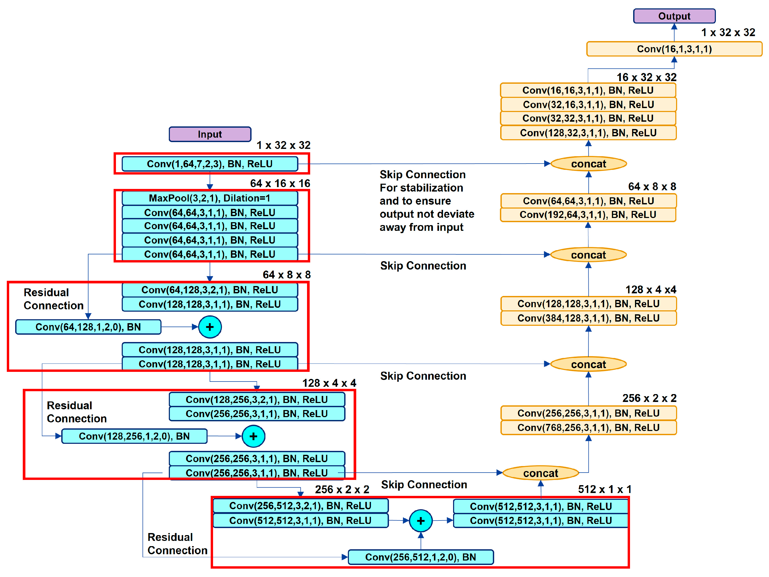
The proposed architecture consists of UNET and RESNET-18 networks for feature extraction, followed by a series of 5 dense layers for classification and dimensionality reduction, as shown in
Figure 2. For the feature extraction part, the input dimension is 1 × 32 × 32. The first block permits the input into down-sampling trend and comprises one convolutional layer with 64 channel features, and 7 × 7 filter kernel and strides 2, followed by batch normalization and rectified linear unit (ReLU) activation function. This produces an output dimension of 64 × 16 × 16. The second block consists of a max pooling layer with 3 × 3 filter kernel and strides 2, followed by 4 convolutional layers where each layer comprises of 64 channel features, and 3 × 3 filter kernel and strides 1, along with batch normalization and ReLU activation in which the output dimension is reduced to 64 × 8 × 8. The third block contains 4 convolutional layers; the first layer comprises 128 channel features, and 3 × 3 filter kernel and strides 2, along with Batch normalization and ReLU activation. The output from the second layer is concatenated with another convolutional layer of 128 channel features, 1 × 1 filter kernel and strides 2, along with Batch normalization, that act as identity mapping to establish a skip connection. The output dimension from this block is further reduced to 128 × 4 × 4. The same process from the third block is repeated for fourth and fifth blocks, which further reduces the output dimension while increasing the channel features to 256 × 2 × 2 and 512 × 1 × 1, respectively. Similarly, the decoder section also consists of 5 residual blocks. Each block permits the input into up-sampling trend and poses a similar number of convolutional layers as the respective encoder block with the same number of channel features and filter kernels, along with batch normalization and ReLU activation, but the strides remain 1 since we expand the output dimension. After passing each decoder block, the number of feature maps are reduced to half and appended by the feature maps’ output from the corresponding encoder block, which acts as an identity mapping to establish skip connections among sections. The output dimension of the decoder section is similar to the input dimension i.e., 1 × 32 × 32.
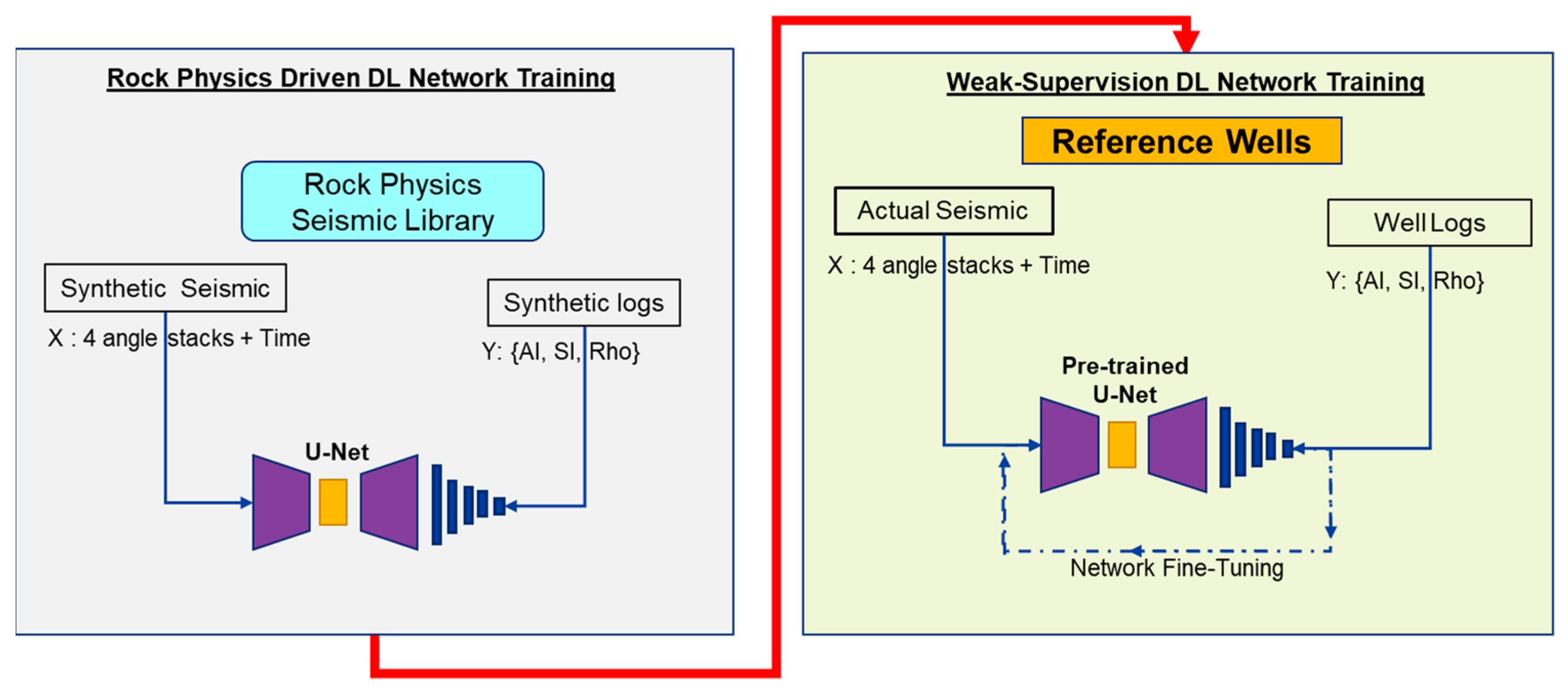
The training was done in 2 steps, as shown in
Figure 3. The first step is called rock physics driven training that trains the network to apprehend the behavior between seismic amplitude characteristics and various rock physics combination possibilities [
13,
14]. The input, X, is the synthetic seismic gathers in 32 sample mini sequences and the output, Y, is the pseudo-elastic properties logs of density, P, and S-Impedance at a mid-point of the mini-sequences. The second step, on the other hand, is called weak supervision training. The weak supervision idea was adopted from tensor flow in transfer learning and fine-tuning tutorials to ascertain that the weakly supervised network undertakes the transfer learning process to recognize the unique character of actual seismic data, i.e., amplitude noise and scaling, attenuation, phase rotation, etc., which is based on the rock physics combination of actual logs at the reference wells. Here, the input, X, is the actual seismic and the output, Y, is the real elastic properties logs taken from 3 actual reference wells.
Prior to the network training, both input X and output Y were scaled using a min-max scaler and simple normalization respectively, to ensure faster convergence during network training optimization. During training, we used the learning rate of 0.0001 with a cosine scheduler criteria for a more efficient convergence. We implemented the mean-square error (MSE) loss function to estimate the error of a set of weights in a neural network, since we are dealing with regression problems to predict pseudo elastic logs. We utilized the ADAM optimization algorithm to update the model weights during backpropagation and the ReLU activation function [
27] to introduce a nonlinear transformation during network training. We also set the epoch hyperparameter to 100, the first 50 epochs mainly focused on the rock physics part. Meanwhile, the next 50 epochs focused on the weak supervision part, utilizing a pre-trained network from the first part training as a base model to further fine-tune and update the model weights within the network [
28]. Finally, we selected the best model at the end of the training and used it as blind testing on actual seismic survey data to produce pseudo elastic properties volumes of density, P, and S-Impedance. To demonstrate that our proposed method works well, we also performed a conventional seismic pre-stack deterministic inversion using the same 3 reference wells and seismic survey data and conducted comparison exercises between both inversion results.
4. Results and Discussion
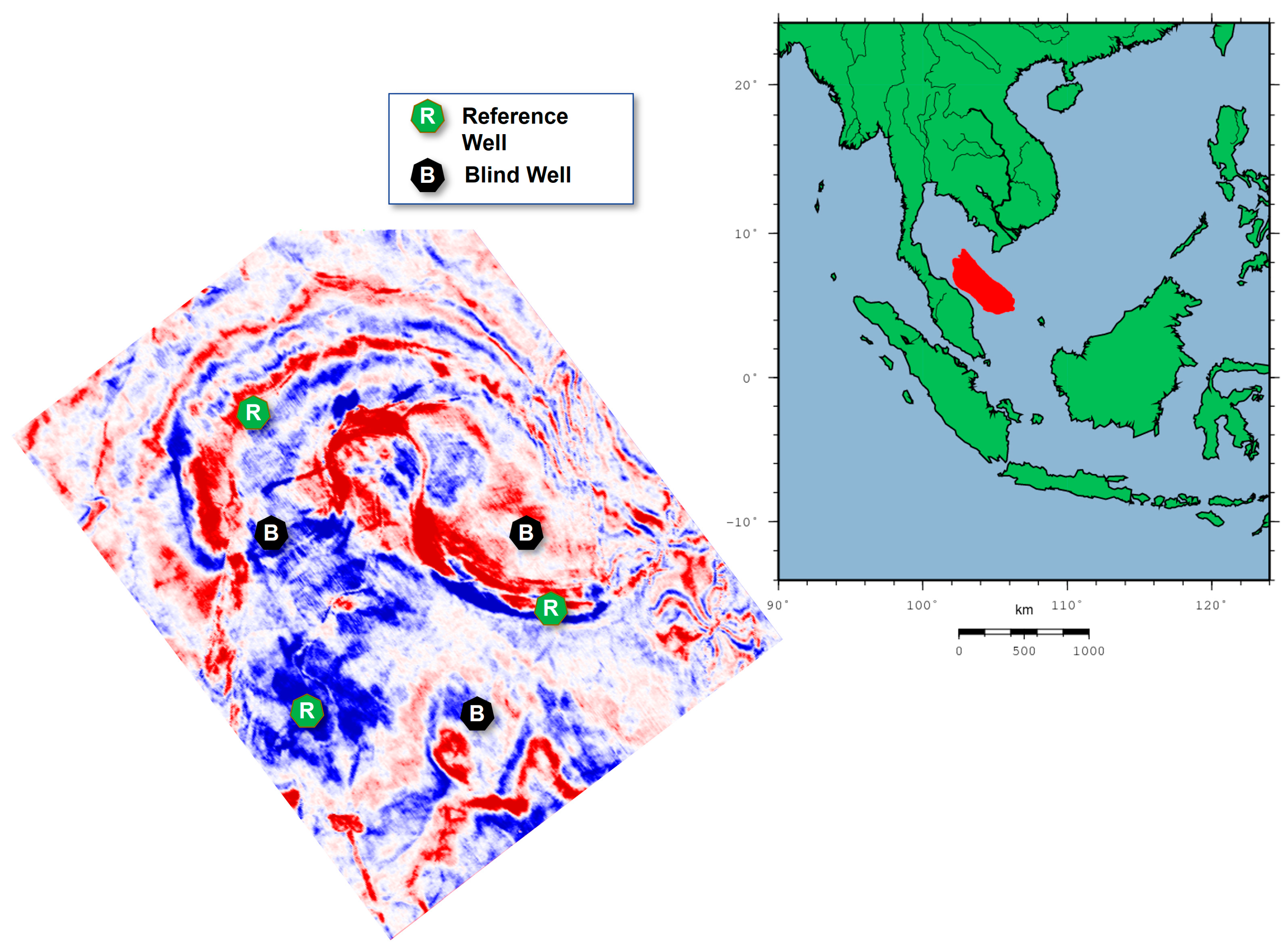
To evaluate the effectiveness of the proposed method, we have conducted blind testing by utilizing actual seismic data from wells from a field in the Malay basin. We gauged the predicted results qualitatively and quantitatively. The qualitative analysis was conducted by examining the background trend fitting and relative variation between predicted and actual elastic properties logs. Meanwhile, the quantitative analysis was mainly performed via the cross-correlation method to estimate correlation accuracy between predicted and actual elastic properties logs.
Figure 4 exhibits the Loss vs. Epoch diagnostic cross plot between training and validation loss trends for the network training. The training loss indicates the adaptability of the network model to fit the training data. In contrast, the validation loss indicates the flexibility of the trained network model to fit the new data. In general, a very good network model performance was observed for training and validation Loss trends for each elastic property, as the trends decrease with an increase in Epoch trends and start to stabilize around some point. Only marginal error contrast between validation and training trends was observed.
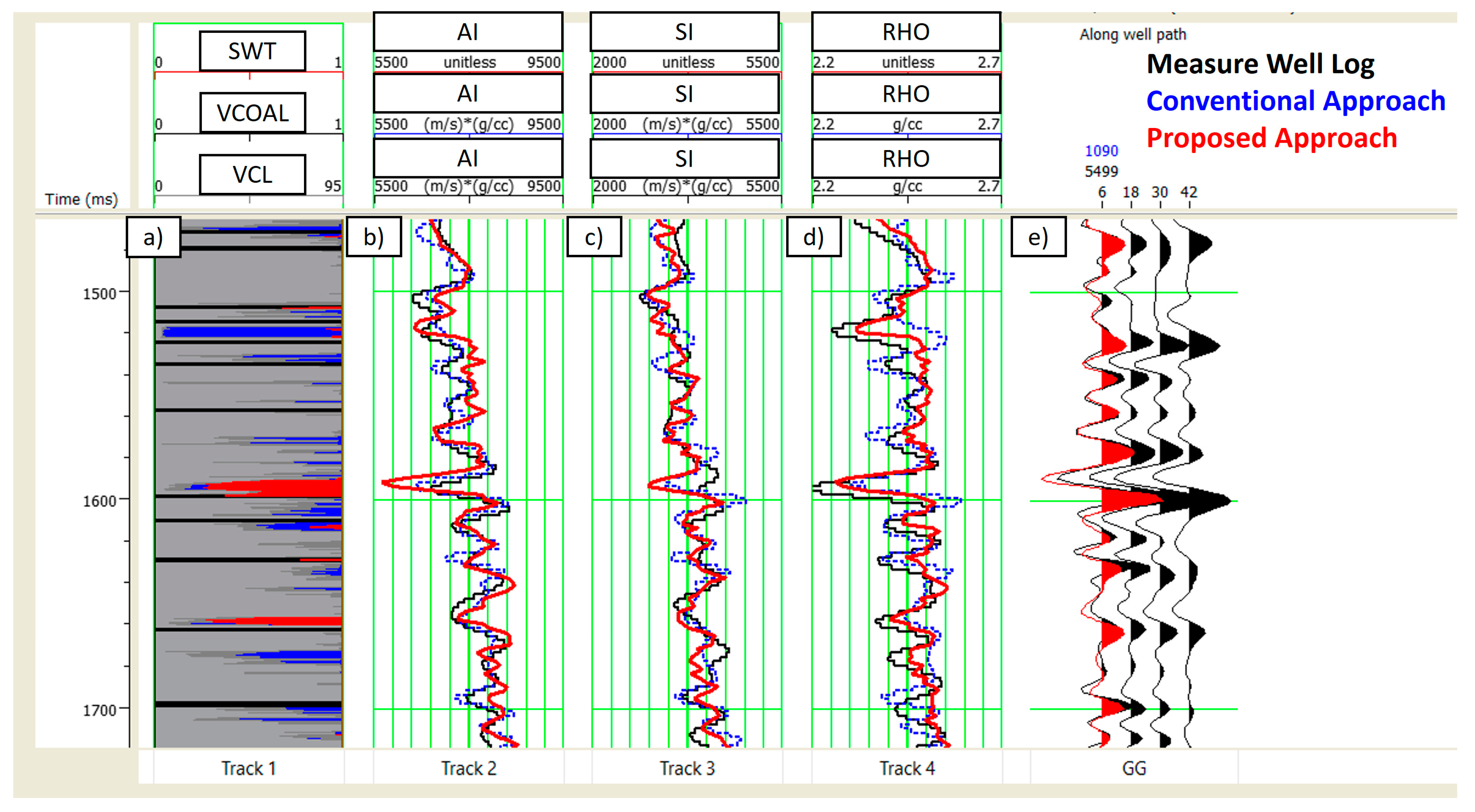
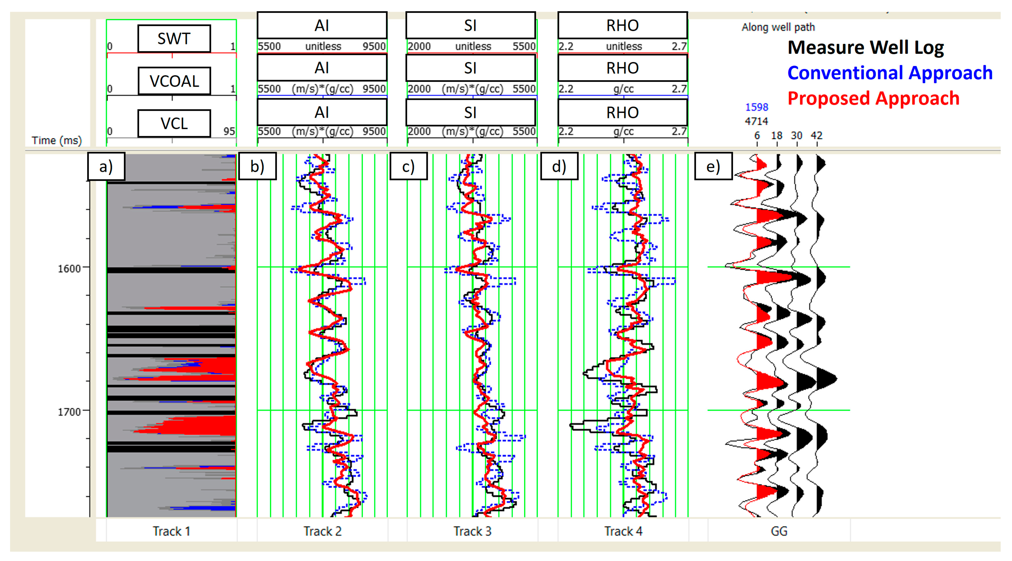
Figure 5 and
Figure 6 demonstrate the well section window for the prediction results from two actual blind wells. The first column represents the litho-fluid log, which comprises the logs’ normalization between clay volume, coal volume, and water saturation. The grey, blue, red, and black colors indicate clay, brine sand, hydrocarbon sand, and coal, respectively. The second column is P-Impedance, the third column is S-Impedance, and the fourth column is density. In each of these columns, the black line indicates the measured elastic properties logs, the blue line is the inversion results from the conventional approach, and the red line indicates inversion results from the proposed approach. The last column is actual seismic pseudo-gathers used as input for inversion. Overall, moderate to good correlation accuracy can be observed between measured elastic properties predicted and predicted elastic properties from both approaches qualitatively. Both approaches can capture the background trend and detect the relative variation of each elastic property. However, the inversion results from the proposed approach are relatively more stable, with less presence of ringing noises and closer proximity to the measured well logs compared to the inversion results from the conventional approach, where many mismatches and ringing noises were observed.
Table 1 demonstrates the correlation accuracy between inversion results and measured logs for both approaches at blind well 1 and 2. There are significant improvements of up to 31% in correlation accuracy for elastic properties prediction based on the proposed approach compared to the conventional, especially for density. This indicates that the trained network model can efficiently capture the background trend and relative variation with proper magnitude and scaling for all elastic properties.
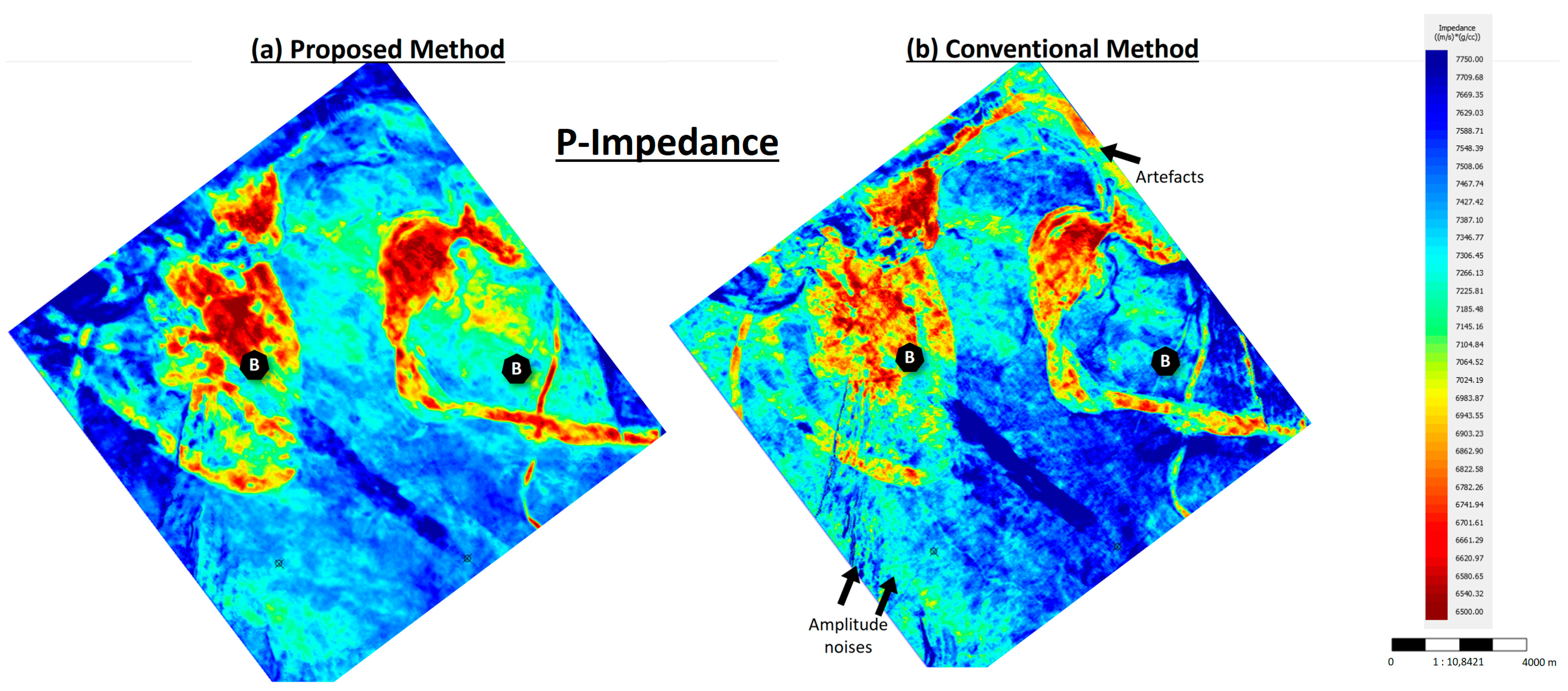
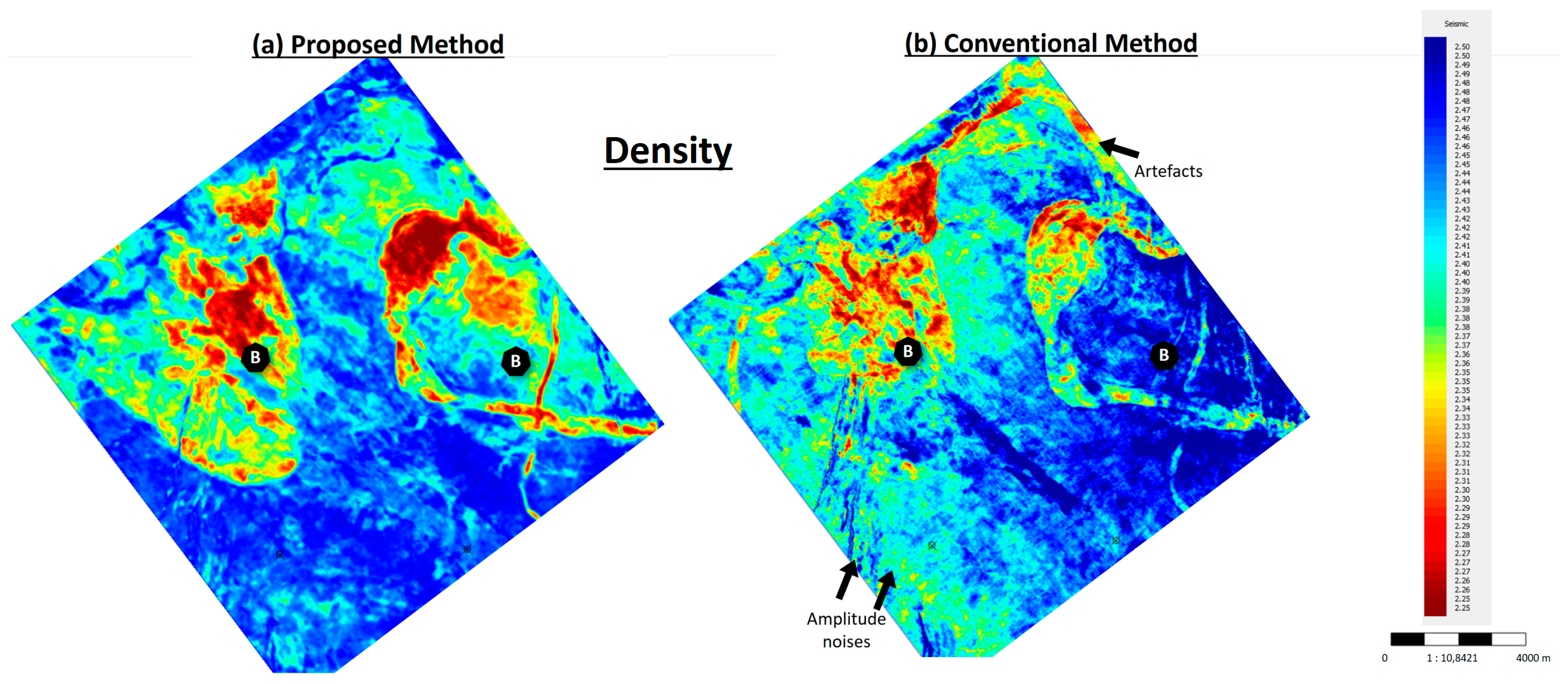
Figure 7 and
Figure 8 demonstrate the map view of the seismic inversion results of P-Impedance and density from both methods at the specified reservoir interval. Both outcomes are encouraging, comparable, and able to highlight the reservoir presence and distribution.
However, the conventional method reveals the presence of scattered amplitude noises and prominent seismic imprints masking the reservoir, especially for density results. The proposed method, on the other hand, produces inversion results with a more stable, clearer definition and fewer noises. This is accomplished without the use of an initial model or wavelet extraction, unlike the standard approach.
Despite better correlation, it is observed that the trained network model cannot accurately capture the relative variation closer to the actual elastic properties. This may indicate that the full correlation between the rock-physics driven synthetic data and real data used was not contextualized during the training. The unique characteristic signatures of synthetic and real seismic and well logs’ data need to be investigated further. The introduction of noise modeling in catching the unique difference between synthetic and real data into the deep learning training process may be useful for prediction accuracy enhancement. In addition, the generation of rock-physics-driven synthetic data library may need to be refined. The current data simulation approach is only limited to two predominant facies. Utilization of more geologically realistic facies into the modeling can aid in establishing more realistic subsurface conditions and potentially enhance prediction accuracy. The approach also could be further improved by incorporating spatial neighboring input data for network training, since the current approach is only limited to trace-based input training. In doing so, the deep neural network may not only comprehend the relationship between seismic and rock physics but also be capable of capturing the structural and stratigraphical information of the subsurface. Aside from spatial-based input training, exploring more complex image-based deep learning algorithms techniques such as Generative Adversarial Networks (GAN), Graphomer, Etc., might also enhance the accuracy estimation.
5. Conclusions
We have successfully developed a new approach of deep learning-based seismic inversion by incorporating seamlessly the rock physics model to generate a vast amount of synthetic pseudo rock properties and their seismic responses. The rock physics library plays a significant role as a comprehensive synthetic dataset input for network training, validation, and testing. Meanwhile, the complex deep learning network architecture, which includes a weakly supervised network, has proven to be useful to enhance computational work efficiency and prediction accuracy while handling data non-linearity and the non-uniqueness of the solutions.
Application of the proposed method on the clastic fluvial-dominated region in the Malay basin reveals the applicability of the method for accurate rock properties prediction. Comparison with the conventional method demonstrated the advantage of the proposed deep learning-based inversion in identifying the reservoir occurrence and distribution. The conventional method exhibited the presence of scattered amplitude noises and prominent seismic imprints masking the reservoir, whereas the proposed method showed more stable and less noises inversion results, yet with faster turn-around time. There are substantial improvements of up to 31% in correlation accuracy achieved upon implementing proposed method for elastic properties prediction compared to conventional method. The trained network model can apprehend the behavior between seismic amplitude characteristics concerning various rock physics combination possibilities and is competent to recognize the unique characteristics and relationships between actual references seismic and well data during the weak supervision transfer learning process. This implies that the proposed method can provide good elastic properties prediction framework and is able to address data limitation and sparsity issues in typical deep learning-based inversion.
