Deformation Energy Estimation of Cherry Tomato Based on Some Engineering Parameters Using Machine-Learning Algorithms

Abstract

For the design and sizing of equipment and structures in agricultural operations concerning the cherry tomato industry, especially harvesting operations and postharvest operations of the crops, it is very important to determine their mechanical properties. In the study, mass, length, thickness, width, geometric diameter, sphericity, surface area, rupture force, firmness, Poisson’s ratio, and modulus of elasticity were used as independent variables in the data set, and the dependent variable and deformation energy was estimated. Min–max normalization methods were used to increase the success and performance of the models. Three machine learning methods were utilized in the study, and statistical parameters, such as R², MAE, and MSE, were used to evaluate the performance of the methods. The R² of the artificial neural network (ANN), applied in the model as one of the machine learning methods, was found to be 96.8%, revealing the highest predictive power. Logistic regression with a 91.1% success rate, and decision tree regression with an 81.3% success rate, came second and third, respectively.

1. Introduction

The cherry tomato (Solanum lycopersicum) is a food product that requires attention at every stage of the chain, from harvest to the consumer, and is very sensitive to external mechanical forces during harvest and postharvest processing. Therefore, it is very important to know its mechanical properties [1]. It is crucial to determine the behaviors of fruit in the face of external forces and to be informed concerning their mechanical properties to increase product quality and contribute to its economic value by minimizing damage and product loss that may occur in the fruit during and after harvest, to make harvest and postharvest processes more efficient, to optimize existing tools, equipment, machinery, and systems for harvest and postharvest processes, and to design new systems [2,3]. The calculation of the mechanical properties of fruits under static and dynamic loading aims to reduce mechanical damage during harvesting, processing, storage, and transport and to specify design parameters for harvesting and storage stages [4,5].

Many researchers and studies have been carried out to determine the mechanical properties of the cherry tomato varieties. Polat et al. (2007) [6] experimented with determining some mechanical properties of cherry tomatoes, such as hardness and coefficient of friction. According to Li et al. (2012) [7], the compressive failure stress of mesocarp and gel tissues was 0.726–0.846 MPa and 0.048–0.124 MPa, respectively. Mahmoud et al. (2022) [8] found the lowest static coefficient of friction on plywood surfaces (0.242) and the highest value on stainless steel surfaces (0.566). The tensile strength and puncture-breaking force of tomato skins vary with peel thickness, as shown by Hetzroni et al. (2011) [9]. Alkali et al. (2014) [10] utilized an artificial neural network (ANN) to predict some mechanical properties of melon fruit. As a result of the experiments, they announced that the values predicted by ANN and the experimental results were compatible up to 95%. Li et al. (2021) [11] used an expanded finite element model to show that the exocarp’s and mesocarp’s fracture mechanical properties play a major role in determining the crack propagation length of tomato fruit. The mechanical properties of fruits and stems of two different tomato species at the light red ripeness stage, including flexural, compression, and tensile properties, were determined by Liu et al. (2021) [12]. Cevher and Yıldırım (2022) [13] estimated the rupture energy values of Deveci and Abate Fetel pear fruit using an artificial neural network (ANN).

As can be seen from the literature review, determining the mechanical properties required for the design and optimization of the machines required for both product quality and product processing is generally carried out destructively under laboratory conditions. These methods are rather costly, labor-intensive, and involve a very long and laborious process. In addition, since the tests are carried out destructively, there is also product waste. In this era, when economy, energy, labor, and time are very important, unconventional non-destructive methods can be used instead of experimental methods to determine these desired properties accurately. Machine Learning is the modeling of systems that make predictions by making inferences on data with mathematical and statistical operations on computers. It is a sub-branch of artificial intelligence science. It contains many methods and algorithm structures [14]. Machine learning has enabled many technological advances, including voice and pattern recognition, data analysis, and prediction. Machine learning, which can learn and develop automatically based only on experience without external intervention, can classify and estimate using training data [15].

Knowing the deformation energy allows the product to be processed with a minimum bruise rate so that it is exposed to minimum damage during harvest and postharvest processing. This study presents an accurate prediction of the deformation energy of cherry tomatoes reliant on some engineering parameters using machine learning. By using machine learning models, it is targeted to determine the most accurate model considering different inputs and network structures. The results obtained can be considered an efficient tool to deal with harvest and postharvest losses of cherry tomatoes and to collect the data necessary for the optimization of existing processing systems and the design of the required machines.

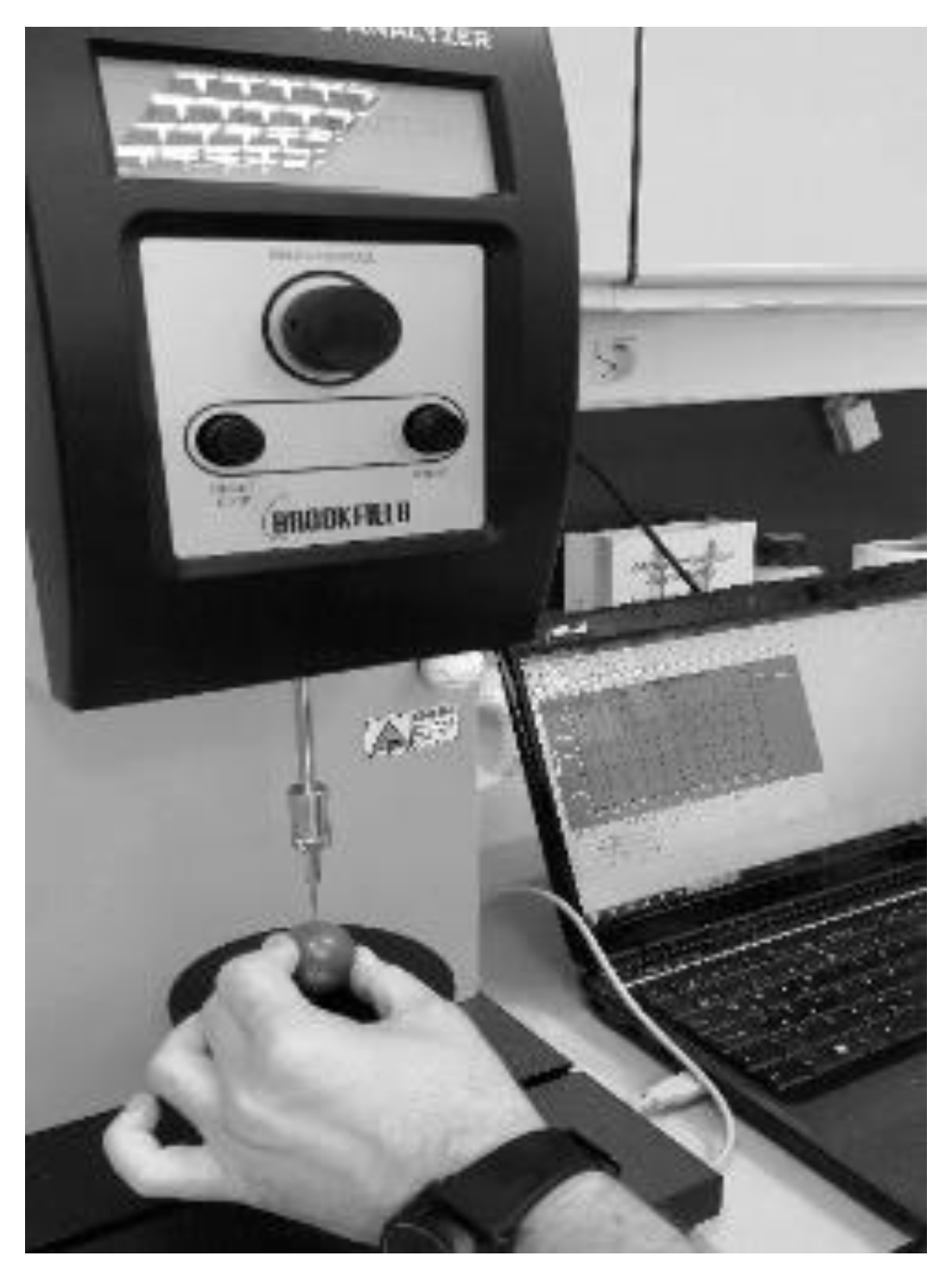
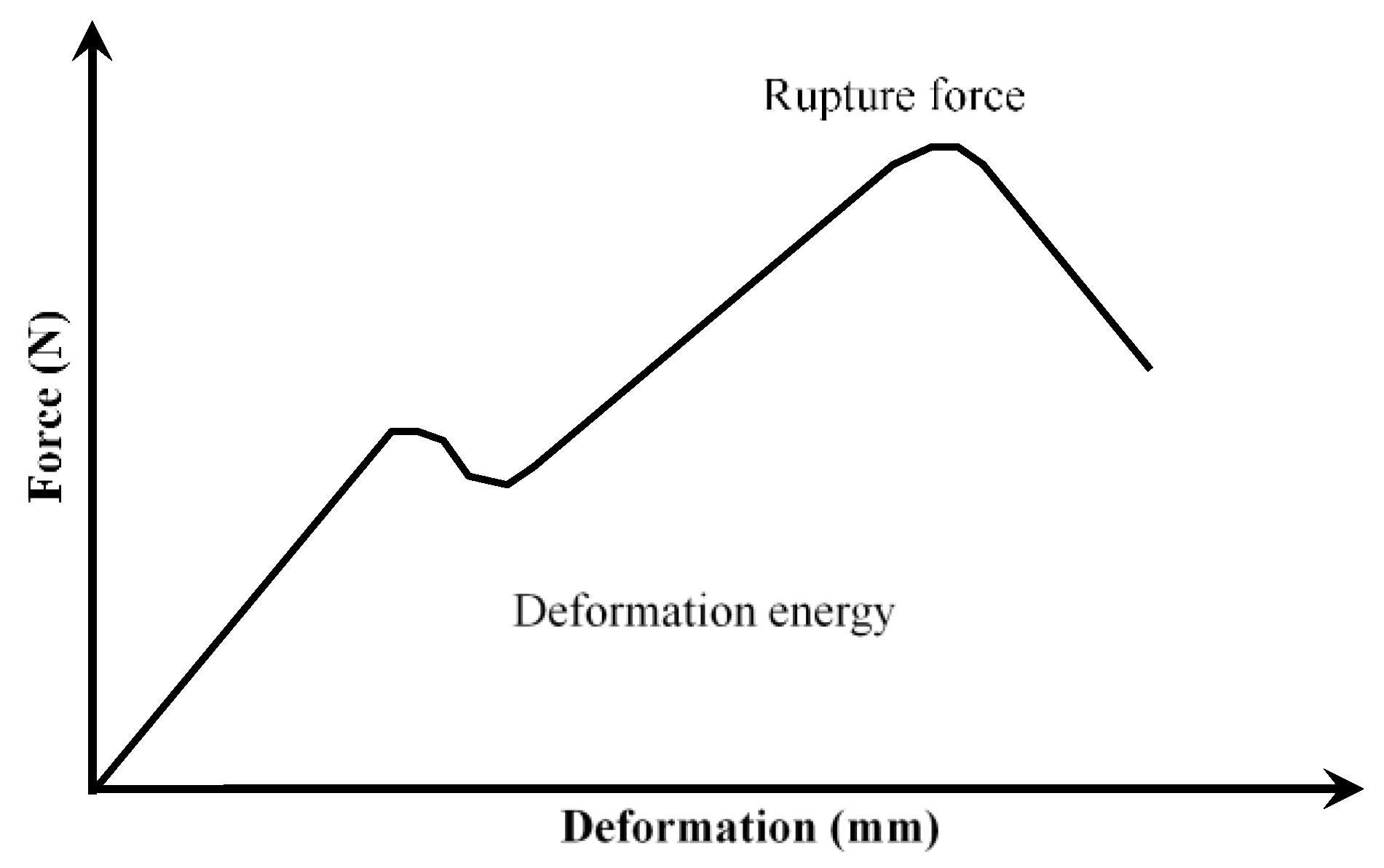
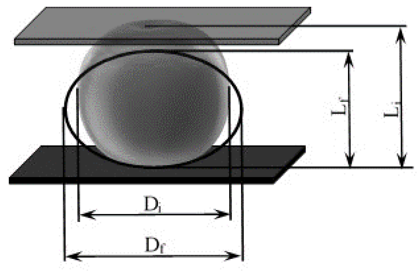
2. Materials and Methods

The cherry tomatoes (Solanum lycopersicum) with a light red ripeness stage used in the experiments were grown and harvested in the greenhouses of Akdeniz University, Manavgat Vocational School in Manavgat, Antalya, in the 2022 harvest season and kept in storage at about 5 °C until laboratory analyses were performed, and tests were implemented after the harvest. The fifteen cherry tomato samples used in the analyses and measurements were randomly selected from the harvested tomatoes. All analyses and experiments were conducted in the laboratories of Akdeniz University Vocational School of Technical Sciences at a room temperature of 20–21 °C over two days.

2.1. Data Set

The physical properties of cherry tomatoes were determined by the following methods: Linear dimensions, i.e., length (L), thickness (T), and width (W), were measured with a vernier caliper with a sensitivity of 0.01 mm, and samples mass (M) was determined using an electronic balance with a sensitivity of 0.001 g [16,17].

The geometric mean diameter, surface area, and sphericity of cherry tomatoes were calculated using the following equations [18]:

$${\mathrm{D}}_{\mathrm{g}}={\left(\mathrm{L}.\mathrm{W}.\mathrm{T}\right)}^{1/3}$$

(1)

$$\mathrm{S}=\mathsf{\pi }.{\mathrm{D}}_{\mathrm{g}}^2$$

(2)

$$\Phi ={\mathrm{D}}_{\mathrm{g}}/\mathrm{L}\times 100$$

(3)

where D_g is the geometric mean diameter (mm), L is the length (mm), W is the width (mm), T is the thickness (mm), S is surface area (mm²), and Φ is sphericity (%).

To determine the rupture force and deformation energy of cherry tomatoes in compressive tests, a biological material test device was utilized (Figure 1).

A curve-ended cylindrical probe 5 mm in diameter was chosen to compress the fruit at a 10 mm min⁻¹ loading velocity during all the tests [19]. The rupture force and deformation energy were found from the force-deformation graph recorded on the computer during the compression test. The area under the force-deformation graph represents the deformation energy, and the peak of the graph gives the rupture force (Figure 2).

After measuring the initial length and width of the fruit, it was forced until deformation occurred on the fruit body (Figure 3). The Poisson ratio (λ) of the fruit was calculated by using the following formula by measuring the final diameter and length after deformation [16]:

$$\mathsf{\lambda }=\mathsf{\Delta }\mathrm{D}/\mathsf{\Delta }\mathrm{L}=({\mathrm{D}}_{\mathrm{i}}-{\mathrm{D}}_{\mathrm{f}})/\left({\mathrm{L}}_{\mathrm{f}}-{\mathrm{L}}_{\mathrm{i}}\right)$$

(4)

where D_i is the initial diameter (mm), D_f is the final diameter (mm), L_i is the initial length (mm), and L_f is the final length of the fruit (mm).

The modulus of elasticity (E) in N mm⁻² of the test fruits was calculated using Boussinesq techniques as follows [3,16]:

$$\mathrm{E}=\mathrm{F}\left(1{-}^2\mathsf{\lambda }\right)/\mathrm{d}.\mathrm{D}.\mathrm{r}$$

(5)

where E is the modulus of elasticity in compression (N mm⁻²), F is force (N), λ is the Poisson ratio, ΔD is deformation (mm), d is the diameter of the cylindrical probe (8 mm), and r is the radius of the curvature of the sample (mm).

The firmness of a sample is regarded as the ratio of compressive force to deformation at the rupture point of a cherry tomato. This was counted up using the formula [20]:

$$\mathrm{Q}=\mathrm{F}/\mathrm{D}$$

(6)

where Q is the firmness (N mm⁻¹), F is the rupture force (N), and D is the corresponding deformation at the rupture point (mm).

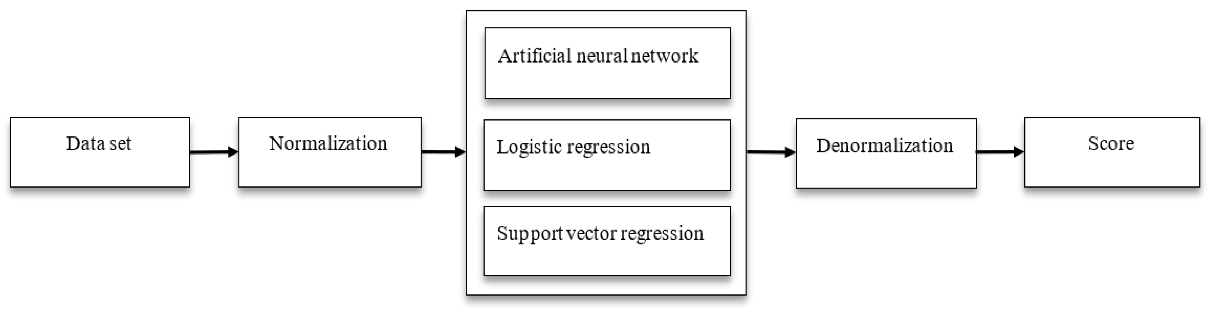
2.2. Machine Learning Methods

Machine learning is the name given to the modeling of systems that make predictions by making inferences on data with mathematical and statistical operations on computers. It solves the problem like a human and provides a gradual solution. It is divided into three categories: Supervised, unsupervised, and reinforced learning. Supervised learning establishes a connection between input and output data. Unsupervised learning is created by using data that is not classified as input data. Reinforcement learning shows how a system that perceives its environment and can make decisions independently can learn how to make the right decisions to achieve its goal [21]. In this study, artificial neural networks, logistic regression, and decision trees from supervised machine learning models were used.

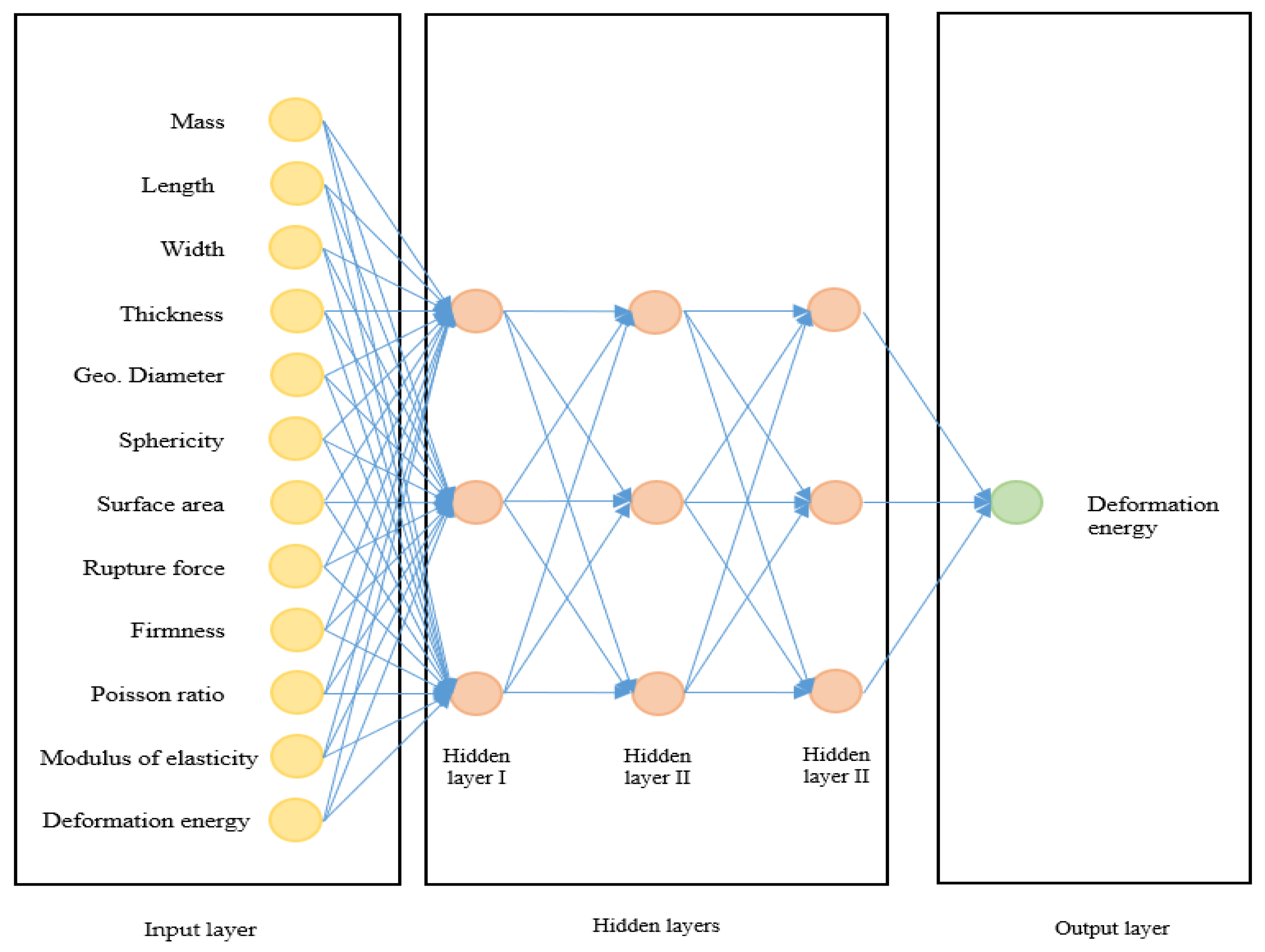
2.2.1. Artificial Neural Networks

Artificial neural networks work similarly to the working structure of the human brain. Artificial neural networks learned through supervised learning can generalize. Artificial neural networks are trained with examples of relevant events and gain the ability to generalize [22].

Artificial neural networks are formed by connecting neurons. It consists of three layers: input, output, and hidden layer(s). Data from the external environment is transferred to the model via the input layer. The data is transmitted to the output layer by training in the hidden layers. Weights are used in the training phase. Weight is the value expressing the effect of the neuron on the system. For the network to be more successful and to show high performance, the weights should be determined correctly. For each neuron, the total function is calculated by multiplying the values of the neurons connected to that neuron by the weight [23].

$$\mathrm{net}={\displaystyle \sum }_{\mathrm{i}=1}^{\mathrm{n}}{\mathrm{w}}_{\mathrm{i}}{\mathrm{x}}_{\mathrm{i}}+\mathrm{b}$$

(7)

Here x represents the input, w represents the weight, and b represents the bias. The output is calculated by passing the sum function through a linear or nonlinear differentiable transfer function. The most commonly used activation functions are linear, sigmoid, ReLu, and tanh [24].

There are types of feedforward and feedback learning in artificial neural networks. In feedforward networks, there is a one-way progression from the input to the output layer. Neurons are arranged in layers. The outputs of the neuron in one layer are multiplied by the weights and given as input to the next layer. In feedback networks, the output of at least one neuron is given as input to itself or another neuron. Feedback can occur between cells in a layer and between neurons between layers. Also, feedback networks show nonlinear dynamic behavior [25].

2.2.2. Logistic Regression

Logistic regression enables determining the nonlinear relationship between the dependent variable and independent variables with two or more categories. It is a method that estimates the probability of occurrence of one of the values the dependent variable can take according to the model created. By making logarithmic transformations, the relationship is transformed into a linear structure, and the probability of certain outcomes for each observation is specified [26].

Since logistic regression is based on probability, the model result obtained should also be in the range of 0 to 1. Probability in logistic regression is expressed as “odds”. Odds are expressed as the ratio of the probability of an event occurring to the probability of it not occurring. The formula is:

$$\mathrm{Odds}=\frac{\mathrm{P}\left(\mathrm{x}\right)}{1-\mathrm{P}\left(\mathrm{x}\right)}$$

(8)

Here, P(x) represents the probability of an event occurring, and 1 − P(x) represents the probability that the event will not occur. The odds ratio ensures that the probability estimation takes a value between 0 and 1, but it should also be ensured that the odds do not take a value below zero. For this, it is necessary to calculate the logit value, which expresses the logarithm of the odds [27].

$$\ln \frac{\mathrm{P}}{1-\mathrm{P}}={\mathsf{\beta }}_0+{\mathsf{\beta }}_1{\mathrm{x}}_1+\cdots +{\mathsf{\beta }}_{\mathrm{k}}{\mathrm{x}}_{\mathrm{ki}}$$

(9)

The logit is negative if the odds are less than 1 and positive if they are larger. The resulting model (the intended model) gathered as a result of logistic regression analysis is a nonlinear logarithmic function, and the coefficients obtained are shown as logarithmic values. Therefore, it is difficult to interpret the coefficients. To interpret these coefficients meaningfully, the odds ratio, that is, the Exponentiated logistic coefficients, is used [28].

$$\ln \frac{\mathrm{P}}{1-\mathrm{P}}={\mathrm{e}}^{\left({\mathsf{\beta }}_0+{\mathsf{\beta }}_1{\mathrm{X}}_1\right)}$$

(10)

2.2.3. Decision Trees Regression

Decision trees are a supervised learning algorithm that can be used for both classification and regression. Decision trees are fruitful in data science as they are easy to understand and interpret and can handle continuous and categorical data. A decision tree is a graphical representation of a set of decisions and the possible consequences of those decisions. It is constructed starting at the root node and progressing through the tree, making decisions based on the values of the properties at each node. The decision tree to be used is selected according to the type of dependent variable. The decision tree model to be used is the classification tree when the dependent variable is categorical, and the model to be used is the regression tree when the dependent variable is continuous [29].

Decision trees are a statistical method. In this method, a tree structure is first created, and the data in the data set is processed into this tree. The structure of decision trees consists of root nodes, nodes, and branches. The root node, the first stage of the tree structure, is created. The root node represents the dependent variable. As you go down the tree structure that starts with the root node, the data sets are divided into small pieces and branches, and new nodes are created. Algorithm selection varies according to the type of target variable. The most frequently used algorithms in decision trees are entropy for categorical variables and Gini for continuous variables; For continuous variables, it is the Least Squares method [30].

In decision trees, the data set is divided into training and testing. Training data is used to create a model. Test data is used to calculate the success and error of the model. If the accuracy is acceptable, the rules are used to predict new data. There are many algorithms used in decision trees. CART, C4.5, C5.0, ID3, and CHAID are the most commonly used [31].

Entropy is a measure of uncertainty. If a dataset has a single label, it has a lower entropy. Therefore, the data should be divided in a way that minimizes entropy. If the splitting process is good, the predictions are successful [32].

$$\mathrm{H}=-\sum \mathrm{P}\left(\mathrm{x}\right)\log \mathrm{p}\left(\mathrm{x}\right)$$

(11)

The information gained is used to determine the best split. Information gain:

$$\mathrm{Gain}\left(\mathrm{S},\mathrm{D}\right)=\mathrm{H}\left(\mathrm{S}\right)-{\displaystyle \sum }_{\mathrm{V}\in \mathrm{D}}\frac{\left|\mathrm{V}\right|}{\left|\mathrm{S}\right|}\mathrm{H}\left(\mathrm{V}\right)$$

(12)

S is the original data set, and D is a partition of the set. Each V is a subset of S. The information gain is defined as the difference between the entropy of the original dataset before the split and the entropy value of each attribute.

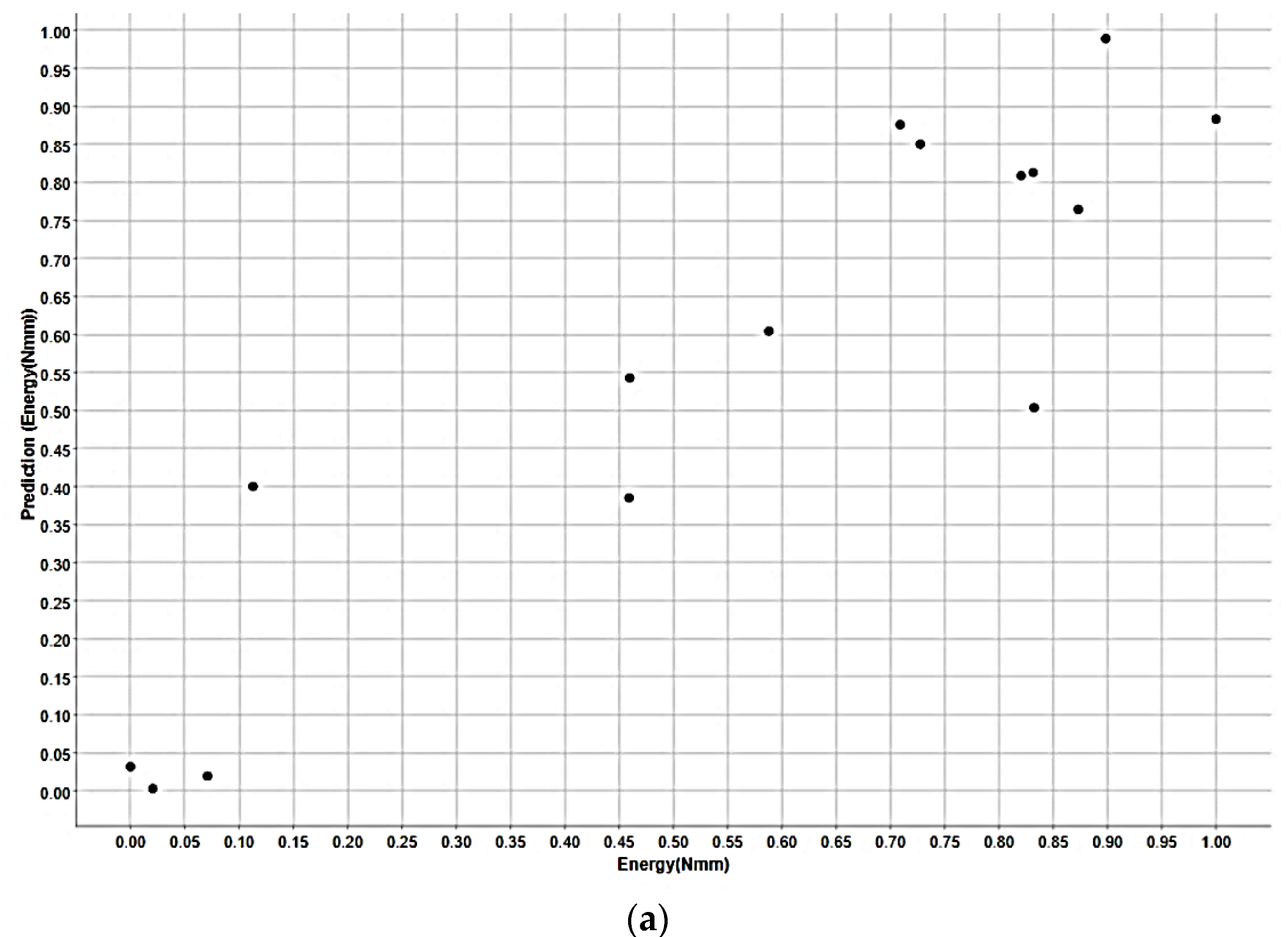
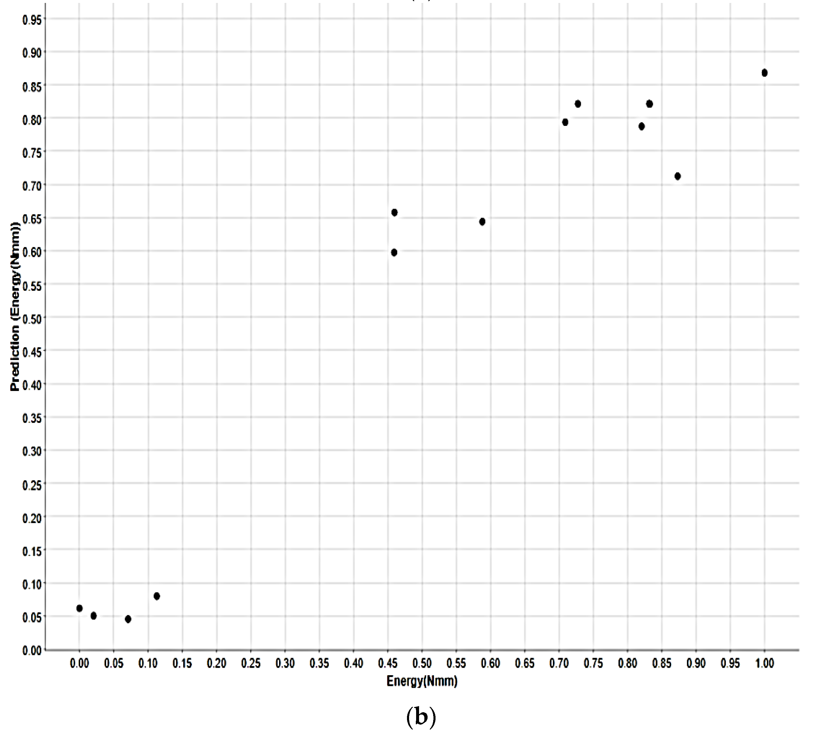
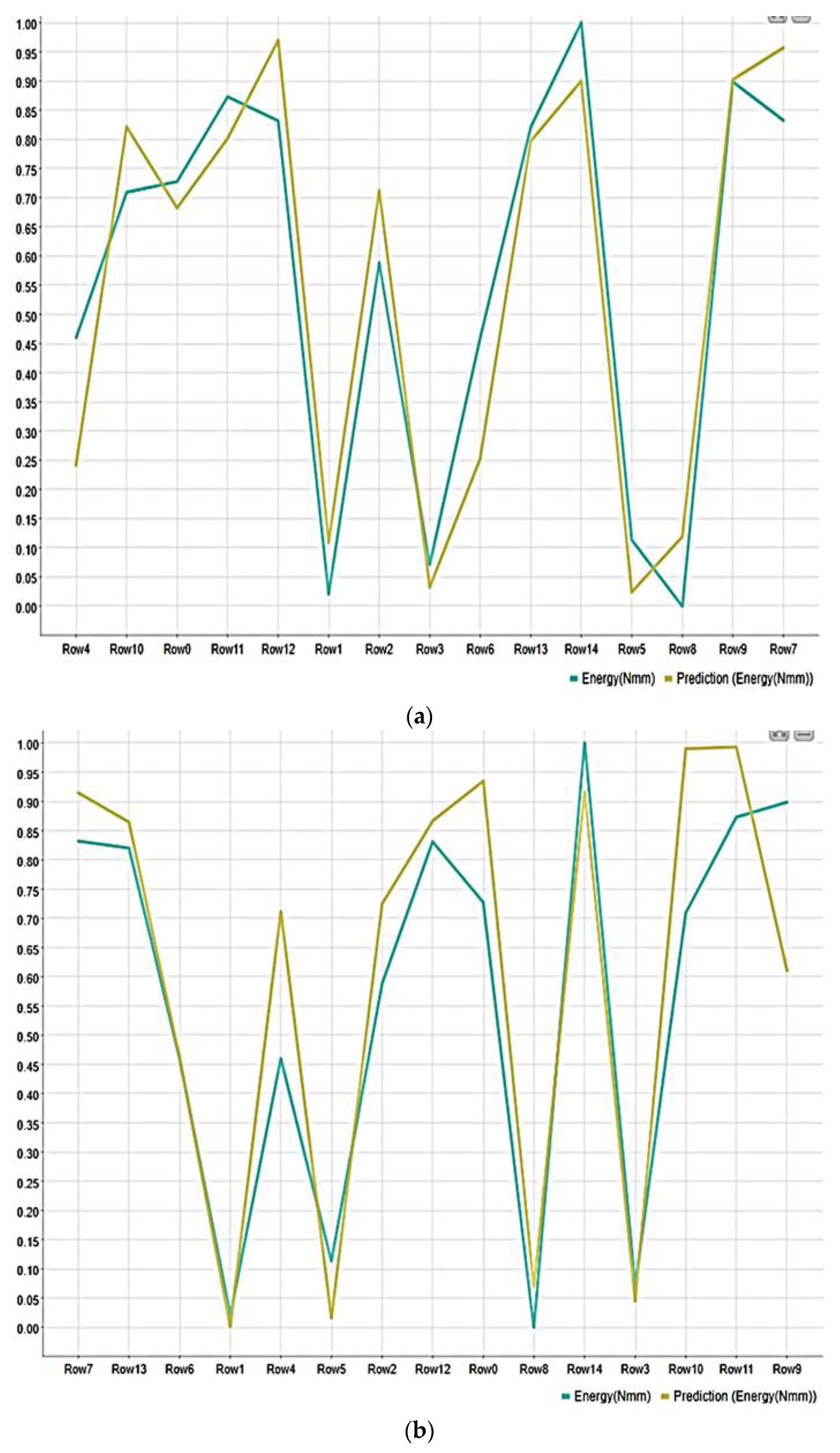
3. Results and Discussion

Conducting modeling studies is crucial in evaluating the mechanical characteristics of fragile and delicate fruit. The statistical summary, including the mean, standard deviation, and ranges of the data utilized for the modeling study, is shown in

Table 1. Experimentally measured physico-mechanical properties of cherry tomatoes.

	Average	Maximum	Minimum	SD
Mass (g)	4.82	7.36	2.48	1.34
Length (mm)	20.90	26.23	16.63	3.43
Width (mm)	17.80	23.27	14.72	3.40
Thickness (mm)	18.43	24.32	15.47	3.08
Geo. Diameter (mm)	18.96	24.50	15.82	3.28
Sphericity (%)	90.65	95.15	86.19	2.58
Surface area (mm2)	1163.61	1886.56	786.94	414.48
Rupture force (N)	23.38	27.61	20.79	1.78
Firmness (N mm−1)	4.97	5.87	4.08	0.64
Poisson ratio	0.29	0.32	0.26	0.02
Modulus of elasticity (N mm−2)	2.59	3.26	1.76	0.51
Deformation energy (N mm)	56.34	70.45	38.36	10.92

.

In the study, three different methods, namely logistic regression, artificial neural networks, and decision trees, were picked to estimate the deformation energy of cherry tomatoes. The working system is shown in Figure 4.

When the figure is analyzed, the first stage is the creation and preprocessing of the data set. In the second stage, normalization operations are performed. It is the method applied to reduce the data set to a certain value range and thus increase the success rate. In the third stage, the machine learning methods used in the study are seen. At this stage, there are three methods: artificial neural networks, logistic regression, and support vector regression. The fourth stage is the denormalization stage, where the actual values of the normalized values are learned. In the last stage, success and error analyses of machine learning models are performed.

Twelve independent variables were used to estimate the deformation energy of cherry tomatoes, the dependent variable of the study. The independent variables of the study were mass, length, thickness, width, geometric diameter, sphericity, surface area, firmness, rupture force, Poisson ratio, and modulus of elasticity. There are 15 data points for each independent variable.

The Min-Max method was used for the normalization of machine learning methods. A linear transformation was performed on the original data. In this normalization, the relationships between the original data values are preserved. This method is a scaling technique in which data is rescaled to be between 0 and 1. For each data set, its minimum value is converted to 0, its maximum value to 1, and all other values in that data set to a decimal between 0 and 1. Having a limited range between 0 and 1 in this process suppresses the effect of outliers and has smaller standard deviations [33]. Min-Max normalization formula:

$$\mathrm{x}\prime =\frac{{\mathrm{x}}_{\mathrm{i}}-{\mathrm{x}}_{\min }}{{\mathrm{x}}_{\max }-{\mathrm{x}}_{\min }}$$

(13)

Here, x is the normalized result, x is the value to be normalized, the smallest value in the x min data set, and the largest value in the x max data set.

In the machine learning model, the data set is divided into two parts, training and testing. Training data is the first data set used to train machine learning algorithms. Models create their rules using this data. The model generalizes by training with the training set and predicts the data it encounters for the first time. Test data is used to evaluate the performance or accuracy of the model. Here, predictions are compared with actual data. It is evaluated by how effective the training is or how accurately the model works. In cases where the results are insufficient, the model’s parameters are changed to give better results in the test. This situation continues until the test result reaches the desired level. The data is usually divided into a 60–70–80% train set and a 40–30–20% test set. There is no definite method for separating the data into training and testing. Here, the best ratio is determined by experimenting with the data set [34,35]. In the study, the data set was divided into two at different rates. The training and test data were divided into two in the ratio of 70–30% because it gave the most successful results resulting from the experiments.

The coefficient of determination (R²), Mean Squared Error (MSE), and Mean Absolute Error (MAE) metrics were calculated to evaluate the machine learning methods.

The coefficient of determination (R²) shows the rate of explanation of independent variables. In other words, it represents the variance ratio of the dependent variable explained by the independent variables. The R² measure is in the range [0, 1]. A coefficient of determination of zero indicates that the independent variables cannot explain the dependent variable at all, while a coefficient of determination of one indicates that they can fully explain the dependent variable. Here, zero indicates that the model has zero explanatory power, and one indicates that the model has 100% explanatory power. According to the calculated R² value, it can be said at what percentage level the independent variables can explain the dependent variable [36]. This value should be close to 1.

$${\mathrm{R}}^2=1-\frac{\mathrm{Unexplained} \mathrm{Variation}}{\mathrm{Total} \mathrm{Variation}}$$

(14)

Mean squared error (MSE) is equal to the mean squared difference between predicted values and actual values. MSE is often used in regression models. Because MSE squares the error, major errors are clearly highlighted. MSE is a metric that ranges from 0 to infinity, and values close to zero are considered better. The lower the MSE value in the calculated MSE values for the same dataset, the more accurate the model is. [37].

$$\mathrm{MSE}=\frac{1}{\mathrm{n}}{\displaystyle \sum }_{\mathrm{i}=1}^{\mathrm{n}}{\mathrm{e}}_{\mathrm{i}}^2$$

(15)

In the formula, n represents the number of data points, and e is the error value.

The mean absolute error (MAE) is calculated by averaging the absolute values of the prediction errors. It is often preferred for determining the error values of the models because it can be easily interpreted. Since MAE is calculated by taking the absolute value of the errors, the direction of the errors is not important. MAE values can vary from 0 to ∞. The lower the MAE value, the lower the error value of the model [38]. The MAE formula is shown in Equation (16):

$$\mathrm{MAE}=\frac{1}{\mathrm{n}}{\displaystyle \sum }_{\mathrm{i}=1}^{\mathrm{n}}\left|{\mathrm{e}}_{\mathrm{i}}\right|$$

(16)

Three different machine learning techniques were used in the study: artificial neural networks, logistic regression, and decision tree regression.

In the artificial neural network method, a feedback model consisting of 11 input neurons and one output neuron was developed. As a result of trial-and-error methods, three hidden layers were used, which was the most successful result. There are three neurons in each hidden layer. The model is shown in Figure 5.

After testing various functions for the activation function, the sigmoid function was preferred because it revealed the most successful result. One of the parameters that affect the success of the model in artificial neural networks is learning. A feedback learning algorithm was used in the study. In this method, 100 iterations were performed. The maximum likelihood method was used to estimate the parameters for the logistic regression model. In the study, the log-likelihood value was −15.882 following 100 iterations. In the decision tree regression used in the study, the Gini index was used as a quality measure, and minimum description length (MDL) was used as a pruning method. The developed models were run 10 times on randomly selected training and test data, and the average was calculated. The evaluation of neural networks, logistic regression, and decision tree regression is given in

Table 2. Success and error evaluation of the models used in the study.

	Artificial Neural Networks	Logistic Regression	Decision Trees Regression
R2	0.968	0.911	0.813
MAE	0.051	0.091	0.097
MSE	0.005	0.011	0.013

.

An R² of 1 indicates that the independent variables are strong in explaining the dependent variable and provide a linear curve. R² was 96.8% for artificial neural networks, 91.1% for logistic regression, and 81.3% for decision tree regression. These results show that the ideal values are met. Mean squared error (MSE) is a statistical metric that evaluates the error values of machine learning methods and shows that values close to zero have fewer errors. An MSE value close to zero indicates that the error is low. It was regarded that the MSE was 0.005 for artificial neural networks, 0.011 for logistic regression, and 0.013 for decision tree regression. The error rate of the models was found to be low and acceptable. The MAE metric gives the magnitude of the error as a quantity. In the study, it was seen that it was 0.051 for artificial neural networks, 0.091 for logistic regression, and 0.097 for decision tree regression. It is accepted that the MAE value is very good in all three models. When evaluated according to error and success values, it is seen that the most successful and least error models are artificial neural networks, logistic regression, and decision tree regression, respectively. Figure 6 shows the scatter plots of the models.

Figure 6 shows the scatter plot of the machine learning models used to estimate the deformation energy of the cherry tomatoes. In all three models, there is a positive and strong relationship between the actual value and the predicted results of the deformation energy of cherry tomatoes. As the value of one of the variables increases, the other increases and the points cluster near the line. Figure 7 shows the line plots of the models.

Figure 7 indicates the relationship between actual and predicted values. The figures show the relationship is strong for all three models. When the figures are analyzed in detail, it is seen that the model with the strongest relationship is artificial neural networks. Then, logistic regression and decision trees are viewed, respectively.

In the literature, it is seen that studies have been carried out using machine learning methods in this field. In most of these studies, the artificial neural network method is used. In this study, logistic regression and decision tree regression methods were also utilized, besides the artificial neural network method. The independent variables used in the model and the parameters of the machine learning models are different. In addition, when the literature is examined, it is obvious that the most successful model is artificial neural networks, with 95% success [11]. In this study, similar to the literature, the most prospering model was artificial neural networks, but the model’s success was 96.8%, which is more successful than in the literature.

4. Conclusions

The physico–mechanical properties of cherry tomatoes are important parameters for harvesting and postharvest operations. These parameters are significant for the design and modification of machines to be used in many processes, such as harvesting, cleaning, sorting, packing, transportation, etc. The determination of these properties requires many samples to be measured over a period of time in order for them to be calculated. It is time-consuming, expensive, and labor-intensive to perform measurements with large numbers of samples. As well as that, several measurement errors are introduced by it. By identifying such features with machine learning, more accurate and faster results will be produced for applications such as discrimination, ranking, and prediction in the industrial sector, as well as larger datasets, attributes, and algorithms that can be used for future research.

In the study, the estimation of the deformation energy of cherry tomatoes was successfully predicted using machine learning methods. Three different supervised machine learning methods, including artificial neural networks, logistic regression, and decision trees, were used in the study. The coefficient of determination (R²), mean absolute error (MAE), and mean squared error (MSE) metrics were calculated to analyze and evaluate these methods. According to the results of the analyses, it was observed that the success rate of all three models was high, and the error was within the acceptable range. Considering the studies in the literature, it is visible that the model is more successful than similar studies. According to the statistical metrics, artificial neural networks, logistic regression, and decision trees were the most successful and least error-prone models for estimating the deformation energy of cherry tomatoes.

References

1. Safitri, Y.; Bintoro, N.; Karyadi, J.N.W. Effect of maturity level and fruit size on mechanical properties of tomato fruit (Solanum lycopersicum). IOP Conf. Ser. Earth Environ. Sci. 2022, 1083, 012063. [Google Scholar] [CrossRef]
2. Hussein, Z.; Fawole, O.A.; Opara, U.L. Harvest and postharvest factors affecting bruise damage of fresh fruits. Hortic. Plant J. 2020, 6, 1–13. [Google Scholar] [CrossRef]
3. Kabas, O.; Ozmerzi, A. Determining the mechanical properties of cherry tomato varieties for handling. J. Texture Stud. 2008, 39, 199–209. [Google Scholar] [CrossRef]
4. Akbarnejad, A.; Azadbakht, M.; Asghari, A. Studies of the selected mechanical properties of banana (Cavendish Var.). Int. J. Fruit Sci. 2017, 17, 93–101. [Google Scholar] [CrossRef]
5. Stopa, R.; Szyjewicz, D.; Komarnicki, P.; Kuta, Ł. Determining the resistance to mechanical damage of apples under impact loads. Postharvest Biol. Technol. 2018, 146, 79–89. [Google Scholar] [CrossRef]
6. Polat, R.; Turkoglu, H.; Atay, U.; Pakyurek, A.Y. Some physico-mechanical and chemical properties of cherry tomatoes (Lycopersicon esculentum cv. Forme) grown under greenhouse. Former. Philipp. Agric. 2007, 90, 75–80. [Google Scholar]
7. Li, Z.G.; Li, P.P.; Yang, H.L.; Liu, J.Z.; Xu, Y.F. Mechanical properties of tomato exocarp, mesocarp and locular gel tissues. J. Food Eng. 2012, 111, 82–91. [Google Scholar] [CrossRef]
8. Mahmoud, W.A.E.M.; Mahmoud, R.K.; Eissa, A.S. Determining of some physical and mechanical properties for designing tomato fruits cutting machine. Agric. Eng. Int. CIGR J. 2022, 24, 131–142. [Google Scholar]
9. Hetzroni, A.; Vana, A.; Mizrach, A. Biomechanical characteristics of tomato fruit peels. Postharvest Biol. Technol. 2011, 59, 80–84. [Google Scholar] [CrossRef]
10. Alkali, B.; Osunde, Z.E.; Sadiq, I.O.; Eramus, C.U. Applications of artificial neural network in determining the mechanical properties of melon fruits. IOSR J. Agric. Vet. Sci. 2014, 6, 12–16. [Google Scholar]
11. Li, D.D.; Li, Z.G.; Tchuenbou-Magaia, F. An extended finite element model for fracture mechanical response of tomato fruit. Postharvest Biol. Technol. 2021, 174, 111468. [Google Scholar] [CrossRef]
12. Liu, J.; Li, Z.; Li, P. The physical and mechanical properties of tomato fruit and stem. In Rapid Damage-Free Robotic Harvesting of Tomatoes; Springer: Singapore, 2021; pp. 127–195. [Google Scholar]
13. Cevher, E.Y.; Yıldırım, D. Using artificial neural network application in modeling the mechanical properties of loading position and storage duration of pear fruit. Processes 2022, 10, 2245. [Google Scholar] [CrossRef]
14. Akmeşe, Ö.F.; Kör, H.; Erbay, H. Use of machine learning techniques for the forecast of student achievement in higher education. Inf. Technol. Learn. Tools 2021, 82, 297–311. [Google Scholar]
15. Baltrušaitis, T.; Ahuja, C.; Morency, L.P. Multimodal machine learning: A survey and taxonomy. IEEE Trans. Pattern Anal. Mach. Intell. 2018, 41, 423–443. [Google Scholar] [CrossRef] [Green Version]
16. Sitkei, G. Mechanics of Agricultural Materials; Akademiai Kiado: Budapest, Hungary, 1986. [Google Scholar]
17. Kabas, O.; Celik, H.K.; Ozmerzi, A.; Akinci, I. Drop test simulation of a sample tomato with finite element method. J. Sci. Food Agric. 2008, 88, 1537–1541. [Google Scholar] [CrossRef]
18. Mohsenin, N.N. Physical Properties of Plant and Animal Materials; Gordon and Breach Press: New York, NY, USA, 1986. [Google Scholar]
19. ASAE S368.2; Agricultural Engineers Yearbook. Compression Test of Food Materials of Convex Shape. ASAE: St. Joseph, MI, USA, 1994; pp. 472–475.
20. Vursavuş, K.; Özgüven, F. Fracture resistance of pine nut to compressive loading. Biosyst. Eng. 2005, 90, 185–191. [Google Scholar] [CrossRef]
21. Bell, J. What is Machine Learning? Machine Learning and the City: Applications in Architecture and Urban Design; John Wiley & Sons: Hoboken, NJ, USA, 2022. [Google Scholar]
22. Jain, A.K.; Mao, J.; Mohiuddin, K.M. Artificial neural networks: A tutorial. Computer 1996, 29, 31–44. [Google Scholar] [CrossRef] [Green Version]
23. Islam, M.M.; Murase, K. A new algorithm to design compact two-hidden-layer artificial neural networks. Neural Netw. 2001, 14, 1265–1278. [Google Scholar] [CrossRef]
24. Basterretxea, K.; Tarela, J.M.; Del Campo, I. Digital design of sigmoid approximator for artificial neural networks. Electron. Lett. 2002, 38, 35–37. [Google Scholar] [CrossRef]
25. Goldman, M.S. Memory without feedback in a neural network. Neuron 2009, 61, 621–634. [Google Scholar] [CrossRef] [Green Version]
26. Schumacher, M.; Roßner, R.; Vach, W. Neural networks and logistic regression: Part I. Comput. Stat. Data Anal. 1996, 21, 661–682. [Google Scholar] [CrossRef]
27. Sperandei, S. Understanding logistic regression analysis. Biochem. Med. 2014, 24, 12–18. [Google Scholar] [CrossRef] [PubMed]
28. Donnelly, S.; Verkuilen, J. Empirical logit analysis is not logistic regression. J. Mem. Lang. 2017, 94, 28–42. [Google Scholar] [CrossRef]
29. Breiman, L.; Friedman, J.; Olshen, R.; Stone, C.C. Classification and Regression Trees; Taylor & Francis: New York, NY, USA, 1984. [Google Scholar]
30. Suárez, A.; Lutsko, J.F. Globally optimal fuzzy decision trees for classification and regression. IEEE Trans. Pattern Anal. Mach. Intell. 1999, 21, 1297–1311. [Google Scholar] [CrossRef] [Green Version]
31. Milanović, M.; Stamenković, M. CHAID decision tree: Methodological frame and application. Economic Themes 2016, 54, 563–586. [Google Scholar] [CrossRef] [Green Version]
32. Wang, L.; Zhou, D.; Zhang, H.; Zhang, W.; Chen, J. Application of relative entropy and gradient boosting decision tree to fault prognosis in electronic circuits. Symmetry 2018, 10, 495. [Google Scholar] [CrossRef] [Green Version]
33. Saranya, C.; Manikandan, G. A study on normalization techniques for privacy preserving data mining. Int. J. Eng. Technol. 2013, 5, 2701–2704. [Google Scholar]
34. Bengio, Y.; Goodfellow, I.; Courville, A. Chapter 1 “Machine learning basics”. In Deep Learning; MIT Press: Cambridge, MA, USA, 2014. [Google Scholar]
35. Jones, D.T. Setting the standards for machine learning in biology. Nat. Rev. Mol. Cell Biol. 2019, 20, 659–660. [Google Scholar] [CrossRef]
36. Ozer, D.J. Correlation and the coefficient of determination. Psychol. Bull. 1985, 97, 307. [Google Scholar] [CrossRef]
37. Wallach, D.; Goffinet, B. Mean squared error of prediction as a criterion for evaluating and comparing system models. Ecol. Model. 1989, 44, 299–306. [Google Scholar] [CrossRef]
38. Chai, T.; Draxler, R.R. Root mean square error (RMSE) or mean absolute error (MAE)?—Arguments against avoiding RMSE in the literature. Geosci. Model Dev. 2014, 7, 1247–1250. [Google Scholar] [CrossRef] [Green Version]
Figure 1. Biological material test device.
Applsci 13 08906 g001
Figure 2. Force-deformation curve of cherry tomato.
Applsci 13 08906 g002
Figure 3. The definition figure of the Poisson ratio.
Applsci 13 08906 g003
Figure 4. The steps of the study in stages.
Applsci 13 08906 g004
Figure 5. ANN model used in the study.
Applsci 13 08906 g005
Figure 6. Scatter plot for graphical analysis of the results of the machine learning models; (a) Artificial neural network; (b) Logistic regression; (c) Decision tree.
Applsci 13 08906 g006aApplsci 13 08906 g006bApplsci 13 08906 g006c
Figure 7. Line plot for graphical analysis of the results of the machine learning models: (a) Artificial neural network; (b) Logistic regression; (c) Decision tree.
Applsci 13 08906 g007aApplsci 13 08906 g007b