Article

Simulation Study on Axial Location Identification of Damage in Layered Pipeline Structures Based on Damage Index

1
Civil Engineering Institute, Institute of Disaster Prevention, Sanhe 065201, China
2
Key Laboratory of Building Collapse Mechanism and Disaster Prevention, Institute of Disaster Prevention, China Earthquake Administration, Sanhe 065201, China
3
School of Architecture and Civil Engineering, Shenyang University, Shenyang 110044, China
4
School of Civil Engineering, Shenyang Jianzhu University, Shenyang 110168, China
*
Authors to whom correspondence should be addressed.
Appl. Sci. 2023, 13(15), 8850; https://doi.org/10.3390/app13158850
Submission received: 28 May 2023 / Revised: 3 July 2023 / Accepted: 17 July 2023 / Published: 31 July 2023
(This article belongs to the Special Issue Advance of Structural Health Monitoring in Civil Engineering)

Abstract

:
This study investigates the feasibility of identifying the axial position of circumferential defects in laminated pipeline structures based on damage indices. Wavelet packet decomposition is combined with damage indices, and the effects of dual defects with the same circumferential position but different axial positions, as well as dual defects with different circumferential and axial positions, on damage indices are separately studied. Our aim was to determine the potential to use damage indices to identify the axial position of circumferential defects in laminated pipeline structures. ABAQUS finite element analysis software was used to establish models of laminated pipeline structures with single defects and dual defects (with the same circumferential position but different axial positions, and with different circumferential and axial positions). The laminated pipeline structure was composed of a steel pipe (structural layer), a rigid polyurethane foam (insulation layer), and a high-density polyethylene (anticorrosion layer). The received sensing signals were averaged, and subjected to 5-level wavelet packet decomposition, to calculate the damage index values, which were then organized into a damage index matrix. Based on the trend of changes in the damage index matrix, the effects of variations in the number and circumferential position of the defects on the identification of the axial position of the damage were analyzed. The results indicate that the trend in damage index changes is influenced by the number of defects, and the increase in the circumferential distance between the second and the piezoelectric element sensor. This study found that when 1.7 λ P D 3.4 λ , I double   defect   90 ° < I single   defect < I double   defect   0 ° ; when 3.7 λ P D 4 λ , I double   defect   90 ° < 0.3 < I double   defect   0 ° < I single   defect . This article demonstrates that the identification of the axial position of damage in laminated pipeline structures can be achieved using the damage index values in the damage index matrix. Additionally, this damage identification method overcomes the limitation of the wavelet packet’s inability to identify dual defects with relatively small relative axial distances. This provides new ideas and methods for finite element analysis in identifying the axial position of damage in laminated pipeline structures.

1. Introduction

Pipelines play an important role in urban construction and modern industry, serving as a necessary means for the long-distance transportation of resources. However, due to the complex working environment of pipelines, their structural layers are vulnerable to corrosion, fatigue damage, and other forms of damage, which can cause material leakage, pollute the environment, and pose a threat to human life and property safety. Ultrasonic guided waves can not only detect damage in long-distance pipelines, but also provide a new method for damage detection in pipelines in complex environments, thus contributing to the monitoring of pipeline structural health.
Up until now, scholars have conducted a series of studies on damage detection in single-layer pipeline structures, but the research focus has mainly been on the identification and localization of individual defects. Wang G. [1] verified through a simulation that the elliptical localization method had a higher accuracy when locating damage in circular pipes but, at the same time, it was found that the circumferential localization error was greater than the axial localization error. El Mountassir et al. [2] proposed a method for the damage detection and localization of pipeline structures based on the sparse estimation of the measurement signal, using a reference signal. Damage detection was achieved by calculating the second estimation error of the signal, while localization was achieved through the recursive sparse estimation of the sliding window of the damage signal. Wei R [3] conducted research on the localization and imaging of circumferential defects in pipelines, and achieved the axial localization of damage using the Hilbert transform, providing a high recognition accuracy. However, the complexity of the working environment in pipelines renders them susceptible to multiple defects, leading researchers to investigate the detection of multiple defects in single-layer pipeline structures. Hu X et al. [4] studied dual defects in pipelines, and found that the reflection coefficient is more sensitive to the relative axial distance than the relative circumferential position, with periodic variations. Wen [5] proposed a weak ultrasonic-guided wave detection method based on the Lyapunov exponent of the Lorenz system, and the simulation and experimental results verified that this method could accurately determine the amount and location of damage in pipelines for health-monitoring purposes. Deng W [6] proposed a frequency-domain synthetic aperture focusing technique, based on phase shift, which overcame the limitations of traditional ultrasonic imaging methods in directly reflecting the imaging results of pipeline defects. The method could accurately determine multiple defects in pipelines for health-monitoring purposes. He J. et al. [7] proposed a three-point axial localization method and circular trajectory imaging method for single and dual defect localization and imaging in pipeline segments, using an elliptical localization imaging method, based on a plate structure. The accuracy of the method was verified through simulation and experiments. Zhang D. [8] conducted impact tests on pipelines under different working conditions before and after damage, and the results showed that using the damage index as a damage discrimination index could not only identify the location of a single defect in pipelines, but also recognize multiple damages in pipelines under different service conditions. Ma Q. [9] conducted a defect localization study on dual defects in single-layer pipeline structures under different working conditions, and the results showed that the circumferential distribution map drawn based on the defect echo peak value could identify the circumferential position of dual defects.
In actual engineering applications, pipelines are mostly layered structures, but scholars have mainly focused on single defects [10,11,12], and conducted less research on double defects [13]. The wave packets of the defect reflection waves overlap due to the close distance between double defects, which makes it challenging to identify the defect reflection wave packets, and to determine the axial position of the defects based on the propagation mechanism of guided waves in the pipeline. Therefore, there is a need for new research methods to accurately determine the relative axial position of double defects. Therefore, this study focuses on double defects in layered pipeline structures, and decomposes the received sensor signal average, using the wavelet packet decomposition method to calculate the damage index values, and form a damage index matrix. Through the comparison of the difference in damage index values between single and double defects in the layered pipeline structure, the relative axial position of the defects can be determined. The research results show that using the damage index value as a parameter to locate the relative axial position of defects in layered pipeline structures provides a new approach and method for the localization of multiple defects in engineering applications.

2. Theoretical Basis

2.1. Dispersion Curves

In 1958, Gazis studied the propagation of guided waves in pipeline structures. Subsequently, researchers investigated the propagation of guided waves in pipeline structures based on the principles of elasticity, and discovered that the guided waves satisfied the Navier displacement equilibrium equation during propagation [14].
μ 2 U + λ + μ · U = ρ 2 U t 2
where U denotes displacement, t denotes propagation time, μ and λ are the Lame constants of the pipe material, ρ denotes the density of the pipe material, and ∇ denotes the Laplace operator.
Researchers calculate the dispersion curves of the layered pipeline structure using the displacement equilibrium equation, which includes three modes of guided waves: the longitudinal mode (referred to as L), torsional mode (referred to as T), and flexural mode (referred to as F). As the study focuses on circumferential damage in layered pipeline structures, the L-mode guided waves are more sensitive to such damage, and have less attenuation and a faster velocity in the frequency range of 0 to 100 kHz. Therefore, the study only analyzes the longitudinal mode guided waves, and the dispersion curve is shown in Figure 1.
This paper is based on the concept of weak dispersion [15,16], and Professor Yan Shi’s theory for selecting excitation modes [17]. Following this theory, we chose the L (0,6) [18] mode, with a central frequency of 70 kHz, as the excitation mode, and we generated a 5-cycle single-tone sinusoidal signal. The theoretical group velocity of this mode is 5208 m/s.

2.2. Wavelet Packet Decomposition and Damage Index

To improve signal resolution, Zhang Y and Huang W et al. have conducted numerous studies [19,20,21,22]. With the deepening of research, wavelet packet analysis has gradually become widely used. Wavelet packet analysis can accomplish the effective time–frequency analysis of monitoring signals, by performing the multi-layer and refined decomposition of both the low-frequency and high-frequency parts of the signal. Additionally, it can autonomously select frequency bands that match the spectral characteristics of the monitoring signal, thereby improving the time–frequency analysis effect of the signal.
Due to the many advantages of wavelet packet analysis, it has been widely used in damage identification and localization in structures. Song et al. [23] conducted a study on the damage level of a bridge deck, and combined intelligent aggregates with damage indices. They found that this approach not only allowed for damage localization, but also enabled the identification of the degree of damage. Yan et al. [24] investigated the damage state of reinforced concrete shear walls under cyclic loading, using a damage index based on wavelet packet decomposition. Du et al. [25] applied a wavelet packet decomposition-based damage index to identify damage in single-layer pipe structures, and demonstrated that multiple damage locations could be accurately detected by detecting abrupt changes in the damage indices, within specific regions of the damage index matrix.
For this study, the guided wave signals received at the piezoelectric element were decomposed into five levels using wavelet packet analysis, with the mother wavelet being Doubechies 5 (also known as db5). This resulted in 2n subsets of high- and low-frequency bands. The wavelet packet decomposition tree is shown in Figure 2.
The relationship between the original signal S, and the subset of frequency band signals obtained from the decomposition, can be expressed by the following equation:
S = X 1 + X 2 + + X 2 n   i = 1 , 2 , , 2 5
where i is the frequency based; and X i is the subset of signals in band i obtained after decomposition.
Du et al. [25,26] applied wavelet packet decomposition to study the damage width in single-layer pipe structures, and proposed a new damage parameter, the damage index. The damage index was calculated for different damage scenarios, and was used to construct a damage index matrix, which is formulated by the following equation:
E i = k = 1 k = m X i , k 2
I = i = 1 2 n E k , i E 1 , i 2 i = 1 2 n E 1 , i 2
where k is the number of signal samples in the band; E i is the signal energy in band i; E 1 , i is the wavelet packet energy in the healthy state of the pipe structure; and E k , i is the wavelet packet energy in the damaged state of the pipe structure.

3. Establishing Finite Element Models

Layered pipeline structures are susceptible to corrosion and stress damage, due to their direct contact with, and exposure to, the transported material during material transport. The amount of damage, and the circumferential and axial positions of damage that occurs during use are complex. One typical and urgent issue to be addressed is the difficulty in determining the axial position of defects when double defects occur in layered pipeline structures during engineering applications, and the distance between the defects is relatively close. This is because the wave packets of the defect reflection waves overlap, making it challenging to identify the defect reflection wave packets, to determine the axial position of the defects. To address the above-mentioned issue, this study uses the finite element simulation software ABAQUS to establish a model of a layered pipeline structure. The study analyzes the sensor signals under different damage quantities and circumferential positions, calculates the damage index values, and constructs two-dimensional damage index matrices based on the relative axial position of the damage and the damage index value. Additionally, a three-dimensional damage index matrix is constructed, based on the relative axial position of the damage, the quantity and angle of the damage, and the damage index value. These matrices are used to locate the axial position of defects in layered pipeline structures, based on the damage index values.
The pipeline model established by finite element simulation is a layered pipeline structure composed of a steel pipe structural layer (inner layer), a rigid polyurethane foam insulation layer (middle layer), and a high-density polyethylene anticorrosive layer (outer layer). The material properties of each layer are shown in Table 1. The actuator is composed of 16 piezoelectric elements, which are centrally coupled at a distance of 30 mm from the near end of the steel pipe structural layer. The sensor is composed of four piezoelectric elements, which are centrally coupled at a distance of 600 mm from the near end of the steel pipe structural layer [27]. This arrangement is designed to suppress the generation of other modes [28], and to ensure that the reflected waves from the damage and the reflected waves from the end are separated. All the research in this paper is based on a layered pipeline structure with different relative axial positions of double defects. Lead zirconate titanate (referred to as PZT-4) was selected as the piezoelectric element in the test system. For the sake of brevity and clarity in the text, the layered pipeline structure is referred to as a pipeline structure; the layered pipeline structure with double defects at the same circumferential position but different axial positions is referred to as a pipeline structure with double defects at the same circumferential position; and the layered pipeline structure with double defects at different circumferential and axial positions is referred to as a pipeline structure with double defects at different circumferential positions.

3.1. Single Defect in Pipe Structure

This study focuses on circumferential defects. A circumferential defect was created in the structural layer of the pipeline structure, by cutting out a section with a length of 3/16 of the pipe’s outer diameter circumference, a width of 4 mm, and a depth of 2 mm. A schematic diagram of the circumferential defect is shown in Figure 3. Nine finite element models of single-defect pipeline structures were established, by varying the axial distance between the circumferential defect and the piezoelectric element sensor. Each model had a defect located at a different axial position. The specific working condition parameters for each model are listed in Table 2.
The purpose of these nine finite element models of single-defect pipeline structures, with different axial positions of the defect, was to calculate the damage index values, and compare them with the damage index values obtained from the finite element models of double-defect pipeline structures. This comparison provided the data for studying the discrimination of the relative axial positions of double defects in the pipeline structure, based on the damage index values.
The models were seeded and gridded, and the seed layout size (which can also be expressed as grid size) and number of grids used in this study are presented in Table 3.

3.2. Double Defect Pipe Structure with the Same Circumferential Position

To investigate the feasibility of discriminating the relative axial position of defects in pipeline structures based on damage index values, double-defect pipeline structure models with the same circumferential location were established. To avoid the influence of the different defect sizes on the discrimination of the relative axial distance of double defects, both defects in this study were of the same size, with a length of 3/16 of the pipe’s outer diameter circumference, a width of 4 mm, and a depth of 2 mm. Additionally, the double defects were located on the same generatrix. The specific operating parameters for this condition are presented in Table 4.
The maximum value of L was set to 1800 mm, based on the reflection angle of the second defect. When the axial distance between the second defect and the piezoelectric transducer exceeded 1800 mm, the reflection echo from the second defect (the first reflection) would overlap with the boundary reflection echo (the second reflection), making it difficult to determine the time when the first reflection was received by the piezoelectric sensor. Therefore, the range of the axial distance between the second defect and the piezoelectric transducer was limited to 750 mm to 1800 mm. The defect plane layout of the double defects with the same circumferential position in the pipeline is shown in Figure 4.

3.3. Double Defect Pipe Structure with Different Circumferential Positions

To further investigate the impact of changes in the relative circumferential position of dual defects in pipeline structures on the ability to discern their relative axial positions, the second defect was rotated by 90 degrees in operating conditions 18 to 25, which were obtained based on operating conditions 10 to 17. Both defects were of equal size, with a length of 3/16 of the pipeline outer diameter circumference, a width of 4 mm, and a depth of 2 mm. Please refer to Table 5 for detailed information on the operating conditions.
The defect plane layout of double-defect pipeline structures with different circumferential positions is shown in Figure 5.

4. Results Analysis

4.1. Sensor Signals of Pipeline Structures with Dual Defects at the Same Circumferential Position

In the positioning study of double defects relative to the axial position, the sensing signals extracted from the piezoelectric element sensors were averaged, to avoid the influence of the angle of the arrangement of the sensors. The averaged sensing signals were then subjected to a wavelet packet decomposition, to calculate the damage index values, which were organized into a two-dimensional damage index matrix. The damage index matrix had the axial distance between the second defect and the piezoelectric element as the x-axis, and the damage index value (referred to as I) as the y-axis, as shown in Figure 6.
Figure 6 shows that the calculated I showed periodic variation, with an increase in PD for the working conditions, where the first defect was located at 750 mm from the piezoelectric sensor, and the second defect was located at a distance ranging from 750 mm to 1500 mm from the sensor, and both defects were located on the same bus line (case 10 to case 15). The reason for this phenomenon was that the two defects were located on the same bus line, and the axial distance difference between the defects caused a phase difference between the reflected wave 1 and reflected wave 2 of the second defect. By comparing the variation patterns of the damage index values of the double defects with the same circumferential position within the axial distance range of 750 mm to 1800 mm, with those of a single defect, we could locate the relative axial position of the defects. To investigate the effect of the phase difference on the reflected waves of the defects, we compared the time-domain signals of the sensing signals for case 10 with those of case 11 and case 12, and the results are shown in Figure 7.
From Figure 7, the time at which each wave packet is received by the piezoelectric sensor for case 10, 11, and 12 is shown in Table 6.
Based on Figure 7 and Table 6, it can be concluded from the comparison between case 10 and case 11 that, although the reflected wave of the second defect overlapped with the mode conversion wave or reflected wave 1, the phase difference between them was close to π/2 (the corresponding phase distance was 111 mm), resulting in the coherent cancellation of the waveform of the reflected wave of the second defect. Similarly, from the comparison between working conditions 10 and 12, it can be concluded that, although the reflected wave of the second defect also overlapped with the mode conversion wave, the phase difference between them was close to π (the corresponding phase distance was 221 mm), resulting in the coherent superposition of the waveform of the reflected wave of the second defect. Therefore, it can be concluded that when the phase difference is close to π/2, the reflected waves of the two defects will produce coherent cancellation; when the phase difference is close to π, the reflected waves of the two defects will produce coherent superposition, leading to a periodic variation trend in the damage index values of the double defects.
Hu X. [4] conducted a study on double defects in a single-layer pipeline structure, and found that when the relative axial distance between the double defects exceeded a certain value, the reflected wave packets of the double defects separated, and they could be regarded as two independent single defects. The guided wave wavelength (referred to as λ) was calculated based on the geometric and material parameters of the pipeline structure in this paper. When the relative axial distance between the defects exceeded 1.36λ (specifically, when the first defect was located 750 mm away from the piezoelectric sensor, and the second defect was located more than 1350 mm away from the sensor), the reflected wave packets of the two defects separated, and the reflected wave could be clearly distinguished in the piezoelectric time-domain graph. This meant that the two defect reflection signals could be detected independently in the piezoelectric time-domain graph once the axial distance between the defects was greater than 1.36λ. To validate the accuracy of the above wave packet separation theory, an analysis of the propagation mechanism of guided waves in pipe structures, based on the propagation mechanism of piezoelectric guided waves, was conducted, as shown in Figure 8. Furthermore, an analysis of the time-domain signal of the sensing signal at case 17 (the first defect was located 750 mm away from the piezoelectric element sensor, and the second defect was located 1800 mm away from the sensor) was performed, and is shown in Figure 9.
From Figure 9, it can be observed that the time of the initial wave extracted at the piezoelectric element sensor was t = 1.6 × 10 4 s, the time of the boundary reflection wave 3 was t = 11.5 × 10 4 s, and the time of the first reflection of the second defect was t = 8.9 × 10 4 s. Based on the pulse-echo method and the time-of-flight method, the propagation velocity and the axial position of the simulated wave were calculated, using finite element simulations. The calculated propagation velocity from the finite element simulation showed a low level of error, compared to the theoretical value for the axial distance of the damage, indicating the accuracy of the finite element simulation. The specific values are shown in Table 7.

4.2. Sensing Signals of Dual Defects in Pipeline Structures Can Vary with Different Circumferential Positions

To avoid the influence of the placement angle of the piezoelectric element sensor on the relative axial distance positioning study of pipeline structure defects, the sensing signal extracted at the piezoelectric element sensor was averaged. The averaged sensing signal was subjected to wavelet packet decomposition to calculate the damage index value, which was then used to form a two-dimensional damage index matrix. The damage index matrix had the axial distance between the second defect and the piezoelectric element as the horizontal axis, and the damage index value as the vertical axis, as shown in Figure 10.
It can be observed from Figure 10 that for case 18 to case 22 (where the second defect was located between 750 mm and 1350 mm away from the piezoelectric element sensor, with a relative circumferential position of 90° between the two defects), the damage index value showed a trend of first increasing and then decreasing, with the increase in the axial distance between the second defect and the piezoelectric element sensor. This trend was caused not only by the increase in the relative axial distance between the two defects, but also by the phase difference in the damage reflection echo caused by the change in the relative circumferential position of the damages.
To further analyze the effect of the relative circumferential position of the damage, a comparison was made between case 14 (where the second defect was located 1350 mm away from the piezoelectric element sensor, with a relative circumferential position of 0° between the two defects) and case 22 (where the second defect was located 1350 mm away from the piezoelectric element sensor, with a relative circumferential position of 90° between the two defects), as shown in Figure 11.
Within the time range of 0.00035 s to 0.0009 s, in the amplified time-domain signal, some random wave packets could be clearly observed. This was because the signal in this area not only contained the reflection echoes but also some random signals, but the amplitude of the random signals could be neglected compared to that of the reflection waves. Figure 11 shows that the time and amplitude of the damage reflection echoes (reflection echo 1 and 2 of the first defect, and reflection echo 1 and 2 of the second defect) received by the piezoelectric element sensor changed, and the waveform became more apparent, as the relative circumferential position of the two defects increased (from 0° to 90°). When the relative axial distance of the damages remained unchanged, changing their relative circumferential position would cause changes in the reception time and the amplitude of the damage reflection echoes.

4.3. Discriminative Analysis of the Number of Structural Defects in the Pipeline

To demonstrate the accuracy of the theory that the relative axial positions of defects in pipeline structures can be located based on the damage index value, the damage index values (referred to as I) were compiled into a three-dimensional damage index matrix for pipeline structures with a single defect, two defects at the same circumferential position, and two defects at different circumferential positions. A comparative study was then conducted on the matrix. The damage index matrix had the axial distance between the defects as the x-axis, the number and relative circumferential positions of the defects as the y-axis, and the damage index value as the z-axis, as shown in Figure 12. The double defects at 0° in the figure refer to the two defects at the same circumferential position in the pipeline structure, while the double defects at 90° refer to the two defects at different circumferential positions in the pipeline structure.
To confirm that the damage index can locate the relative axial position of defects in pipeline structures, it can be observed from Figure 12 that a comparison was made between the damage index of a pipeline structure with a single defect, and the damage index (I) of a pipeline structure with double defects at the same circumferential position (referred to as double defects at 0°). The specific research results regarding the relationship between the two with respect to I are shown in Table 8. For ease of analysis in the following discussion, the relative axial distance of the double defects is denoted as “l”.
To study the impact of changes in the relative circumferential position between double defects on the damage index for determining the relative axial position of defects, the damage index values for a single defect ( I signal   defect ) were compared with those for double defects at 90° ( I double   defect   90 ° ) and those for double defects at 0° and 90° ( I double   defect 0 ° and I double   defect 90 ° ). Our study found that when 1.7 λ P D 4 λ , the following relationship always holds between I signal   defect and I double   defect   90 ° : I double   defect   90 ° < I signal   defect . However, there are two differences between I double   defect   0 ° and I double   defect   90 ° , as shown in Table 9.
In summary, based on the range of 1.7 λ P D 4 λ , the changes in the amplitude and increasing/decreasing trend of I with increasing PD can be used for locating the relative axial position of defects in pipeline structures. Furthermore, changes in the relative circumferential position of double defects can have an impact on the amplitude of I, and its changing trend with increasing PD.

5. Experiment

To verify the accuracy of the finite element simulation, and the correctness and applicability of the conclusions in this study, a piezoelectric ultrasonic guided wave damage identification test system was established for a laminated pipeline structure, based on six working conditions in the finite element simulation. The damage index values obtained from the test system were then compared with those obtained from the finite element simulation.
The test system was based on four laminated pipes, and six sets of damage identification tests were conducted. For the reader’s convenience, the working conditions established in the test system have the same numbers as those in the finite element simulation. The information regarding the damage location and other details are shown in Table 10.
The geometric and material parameters of the laminated pipe structure used in the test system were the same as those in the finite element simulation, as shown in Table 1. The radial cross-section of the laminated pipe structure can be seen in Figure 13.
Due to the fact that the laminated pipe structure was covered with an outer layer, piezoelectric sensors were placed at the end of the structural layer, to ensure the integrity of the outer layer. In this test, 12 mm × 6 mm × 1 mm PZT-4 was used as the actuator and sensor, and the number and arrangement of the sensors were the same as those in the simulation.
First, two intact pipeline structures were selected for single-defect tests, such as case 5 and case 8. Based on the single-defect pipeline structures, double-defect tests were conducted at the same circumferential position, such as case 13 and case 16. Then, two intact pipeline structures were selected for double-defect tests at different circumferential positions, such as case 21 and case 24. The circumferential dimensions of the damage studied in the experimental system were consistent with those in the finite element simulation, and the damage schematics are shown in Figure 3. A L (0,6) mode, with a central frequency of 70 kHz and a 5-cycle single-tone sine wave superimposed signal, was selected as the excitation guided wave. The experimental system setup is shown in Figure 14.

6. Verification and Comparison

The sensing signals captured by the sensor array were filtered to obtain clearer sensing signals. The sensing signals of case 13 at the same circumferential position and case 21 at different circumferential positions were decomposed into five levels of wavelet packets, and the specific damage index values were calculated. For case 13 and case 21, the damage index values obtained from the tests were compared with those obtained from the finite element simulation, and the errors between the test and the simulation were calculated. The specific numerical values are shown in Table 11.
As shown in Table 11, the errors between the damage index values obtained from the experiments and those obtained from the finite element simulations were relatively small. This indicated that the finite element simulations could accurately represent the actual behavior of the pipeline structures, and confirmed the accuracy of the simulation model. Therefore, the finite element simulation could be considered a reliable tool for predicting the behavior of pipeline structures in real-world applications.
To validate the accuracy of the conclusions drawn in this paper, we compared the damage index values for a single defect, same circumferential position, and different circumferential position, using the sensor signals obtained from experiments within the range of 1.7λ ≤ PD ≤ 4λ, after a five-level wavelet packet decomposition. The specific damage index values are shown in Table 12.
Based on Table 12, the following relationships between single and double defects can be observed: when 1.7 λ PD 3.4 λ , I double   defect   90 ° < I signal   dafect < I double   defect   0 ° ; when 3.7 λ PD 4 λ , I double   defect   90 ° < 0.3 < I double   defect   0 ° < I signal   defect ; when 1.7 λ PD 4 λ , I double   defect   90 ° < I double   defect   0 ° .
The relationship between single and double defects obtained from the experimental system was consistent with the conclusions obtained from the simulation, which, to some extent, proves the accuracy of the conclusions in this paper.

7. Conclusions

This paper investigated the second defect in laminated pipeline structures, and determined the relative axial position between the first and second defects, based on the damage index value. The relationship between the relative axial position of the damage and the damage index value was obtained through finite element simulation, and the accuracy of this relationship was verified experimentally. The specific relationship can be summarized as follows:
  • When comparing the damage index values (I) of double defects at the same and different circumferential positions with those of single defects in pipeline structures, it was found that within the range of 1.7 λ P D 3.4 λ , the order of damage index values was I double   defect   90 ° < I signal   defect < I double   defect   0 ° . Based on this relationship between the damage index values of double and single defects in pipeline structures within the range of 1.7 λ P D 3.4 λ , simulations were conducted to obtain the damage index value for a single defect. The wavelength λ of the guided wave was calculated using the relevant parameters, and the simulated damage index value was compared with the measured value obtained from actual engineering applications, to locate the relative axial position of the defects. These findings highlighted the importance of accurately detecting and repairing defects in pipeline structures, especially double defects, to ensure their safe and reliable operation.
  • When comparing the damage index values (I) of double defects at the same and different circumferential positions with those of single defects in the pipeline structures, it was found that when 3.7 λ P D 4 λ , the order of damage index values was I double   defect   90 ° < 0.3 < I double   defect   0 ° < I signal   defect . Within the range of 3.7 λ P D 4 λ , the reflected waves from the two defects began to separate. At this point, the relative axial position of the defects could be located through two main methods. Firstly, as the reflected waves from the defects began to separate, the relative axial position of the defects could be calculated using the pulse-echo method. Secondly, based on the relationship between the damage index values of double and single defects within this range, simulations could be conducted to obtain the damage index value for a single defect. The wavelength λ of the guided wave was calculated using the relevant parameters, and the simulated damage index value was compared with the measured value obtained from actual engineering applications, to locate the relative axial position of the defects.
  • In order to investigate the impact of changes in the relative circumferential positions between double defects on the damage index (I) in pipeline structures, we compared the values of I double   defect   0 ° and I double   defect   90 ° . Our study revealed that within the range of 1.7 λ P D 4 λ , changes in the relative circumferential positions of the defects affected the amplitude of the damage index values of double defects, and their changing trends with the increase in L, but did not alter the magnitude relationship between the damage index values of double defects at different circumferential positions, with I double   defect   0 ° consistently being greater than I double   defect   90 ° .

Author Contributions

Conceptualization, Y.L. and L.Q.; methodology, Y.L.; software, L.Q.; validation, Y.L., L.Q. and B.Q.; formal analysis, Y.L.; investigation, L.Q.; resources, Y.L.; data curation, L.Q.; writing—original draft preparation, L.Q.; writing—review and editing, Y.L., L.Q. and B.Q.; visualization, Y.L.; supervision, B.Q.; project administration, Y.L. All authors have read and agreed to the published version of the manuscript.

Funding

This research was funded by the Fundamental Research Funds for the Central Universities, grant number ZY20220201, the Liaoning Provincial Education Department Scientific Research-Youth “Nurturing” Project, grant number 2020JYT06, the Funded by Science and Technology Project of Hebei Education Department, grant number QN2023146, the Langfang Municipal Science and Technology Plan Project, grant number 2022013091, and the Natural Science Foundation of Liaoning Province, grant number 2021-BS-278, Educational Research and Teaching Reform Project of Institute of Disaster Prevention, grant number JY2023A08.

Institutional Review Board Statement

Not applicable.

Informed Consent Statement

Not applicable.

Data Availability Statement

Not applicable.

Conflicts of Interest

The authors declare no conflict of interest.

References

  1. Wang, G.; Li, F.; Liu, Z.; Meng, G. Application of ultrasonic guided waves in damage localization of cylindrical structures. J. Vib. Meas. Diagn. 2017, 37, 440–448+623. [Google Scholar]
  2. El Mountassir, M.; Mourot, G.; Yaacoubi, S.; Maquin, D. Damage detection and localization in pipeline using sparse estimation of ultrasonic guided waves signals. IFAC-Pap. Online 2018, 51, 941–948. [Google Scholar]
  3. Wei, R. Numerical Simulation and Imaging Technology of Guided Wave for Pipeline Damage. Master’s Thesis, Dalian University of Technology, Dalian, China, 2021. [Google Scholar]
  4. Hu, X.; Feng, X.; Zhou, J. Numerical simulation on the interaction of longitudinal guided waves with double defects in pipes. Insp. Integr. 2021, 40, 306–312. [Google Scholar]
  5. Wen, Y.; Wu, J.; Lin, R.; Ma, H. Ultrasonic guided wave detection in a pipeline based on Lyapunov exponent of Lorenza system. J. Vib. Shock. 2019, 38, 264–270. [Google Scholar]
  6. Deng, W.; Long, S.; Chen, X.; Li, Z.; Li, Q. Research on frequency domain synthetic aperture focusing pipeline guided wave imaging based on phase migration. AIP Adv. 2021, 11, 035314. [Google Scholar]
  7. He, J.; Zhou, C.; Yang, L.; Sun, X. Research on pipeline damage imaging technology based on ultrasonic guided waves. Shock Vib. 2019, 2019, 1470761. [Google Scholar]
  8. Zhang, D. Study on stress wave monitoring and damage identification of pipeline based on piezoceramic transducers. Master’s Thesis, Yangtze University, Jinzhou, China, 2021. [Google Scholar]
  9. Ma, Q. Research on buried pipeline damage identification based on ultrasonic guided waves. Master’s Thesis, Yangtze University, Jinzhou, China, 2021. [Google Scholar]
  10. Li, Y.; Yan, S. Behaviors analysis on UGWs propagation in layered pipeline structures with damages. J. Shenyang Jianzhu Univ. 2020, 36, 1074–1081. [Google Scholar]
  11. Yan, S.; Liu, D.; Li, Y.; Cheng, Y. Damage identification for layered pipe structures using piezoelectric guided waves. J. Shenyang Jianzhu Univ. 2016, 32, 619–627. [Google Scholar]
  12. Nakhli Mahal, H.; Yang, K.; Nandi, A.K.; Johnson, L. Improved defect detection using adaptive leaky NLMS filter in guided-wave testing of pipelines. Appl. Sci. 2019, 9, 294. [Google Scholar]
  13. Shao, Y.; Liu, Y.; Su, Z. Detection of defects using spatial variances of guided-wave modes in testing of pipew. Appl. Sci. 2020, 10, 1–14. [Google Scholar]
  14. Yan, S.; He, B.; Zhao, N. Experimental validation and plotting guided wave dispersion curve of pipe structure. Eng. Mech. 2012, 29, 159–163. [Google Scholar]
  15. Chen, Y. Propagation characteristics of piezoelectric ultrasonic guided waves in layered pipeline structure. Master’s Thesis, Shenyang Jianzhu University, Shenyang, China, 2015. [Google Scholar]
  16. Liu, D. Propagation characteristics of piezoelectric ultrasonic guided waves in liquid-filled layered pipeline structure. Master’s Thesis, Shenyang Jianzhu University, Shenyang, China, 2016. [Google Scholar]
  17. Yan, S.; Li, Y.; Zhang, S.; Song, G.; Zhao, P. Pipeline damage detection using piezoceramic transducers: Numerical analyses with experimental validation. Sensors 2018, 18, 2106. [Google Scholar]
  18. Lamb, H. On Waves in an Elastic Plate. Proc. R. Soc. Lond. Ser. A Contain. Pap. A Math. Phys. Character 1917, 93, 114–128. [Google Scholar]
  19. Zhang, Y.; Sun, X.; Zhang, X. Resolution enhancement method of L(0,2) ultrasonic guided wave signal based on variational mode decomposition, wavelet transform and improved split sepctrum processing. Appl. Sci. 2020, 10, 1–17. [Google Scholar]
  20. Huang, W.; Wang, X.; Zhao, J. Enhancement of ultrasonic guided wave signals using a split-spectrum pocessing method. Appl. Sci. 2021, 11, 1–12. [Google Scholar]
  21. Azuara, G.; Ruiz, M.; Barrere, E. Damage localization in composite plates using wavelet transform and 2-D convolutional neural networks. Sensors 2021, 21, 5825. [Google Scholar]
  22. Pedram, S.K.; Gan, T.-H.; Ghafourian, M. Improved defect detection of guided wave testing using split-spectrum processing. Sensors 2020, 20, 4759. [Google Scholar]
  23. Song, G.; Gu, H.; Mo, Y.L.; Hsu, T.T.C.; Dhonde, H. Concrete structural health monitoring using embedded piezoceramic transducers. Smart Mater. Struct. 2007, 16, 959–968. [Google Scholar]
  24. Yan, S.; Sun, W.; Song, G.; Gu, H.; Huo, L.S.; Liu, B.; Zhang, Y.G. Health monitoring of reinforced concrete shear walls using smart aggregates. Smart Mater. Struct. 2009, 18, 3149–3160. [Google Scholar]
  25. Du, G.F.; Chen, G.C.; Jiao, W.S.; Zhang, D. Pipeline damage identification based on piezoelectric ceramic sensor. J. Yangtze Univ. 2021, 18, 109–117. [Google Scholar]
  26. Du, G.; Kong, Q.; Zhou, H. Multiple cracks detection in pipeline using damage index matrix based on piezoceramic transducer-enabled stress wave propagation. Sensors 2017, 17, 1812. [Google Scholar] [PubMed] [Green Version]
  27. Zhang, S. Damage identification analysis and experimental validation of pipeline structures using piezoelectric element. Master’s Thesis, Shenyang Jianzhu University, Shenyang, China, 2017. [Google Scholar]
  28. Lih, S.S.; Rose, J.L.; Qiu, L. A study on the effects of piezoelectric wafer active sensors on Lamb wave propagation in metallic plates and pipes. Smart Mater. Struct. 2004, 13, 779–788. [Google Scholar]
Figure 1. Dispersion curve of the layered pipe structure.
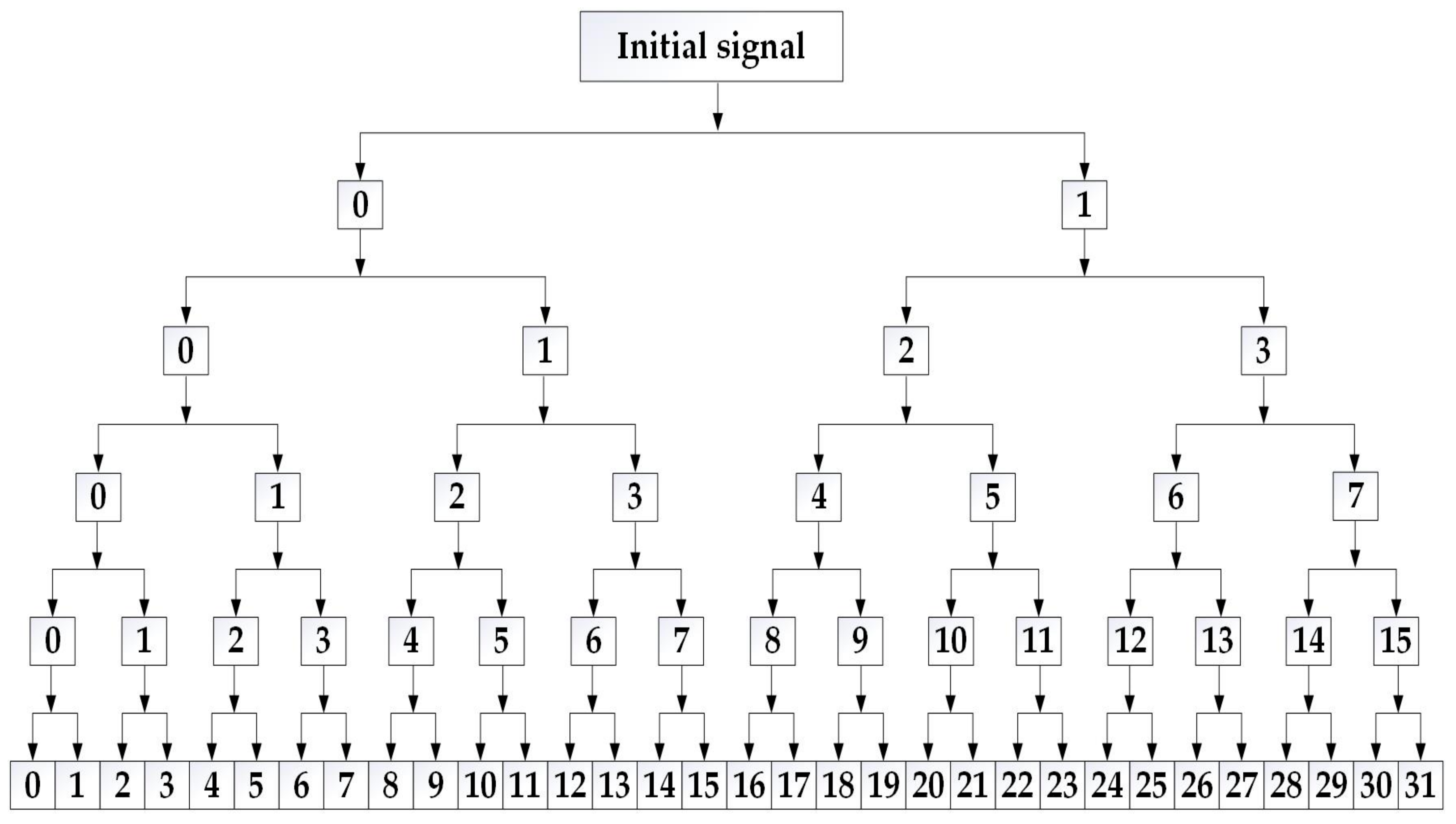
Applsci 13 08850 g001
Figure 2. Wavelet packet decomposition tree at level 5.
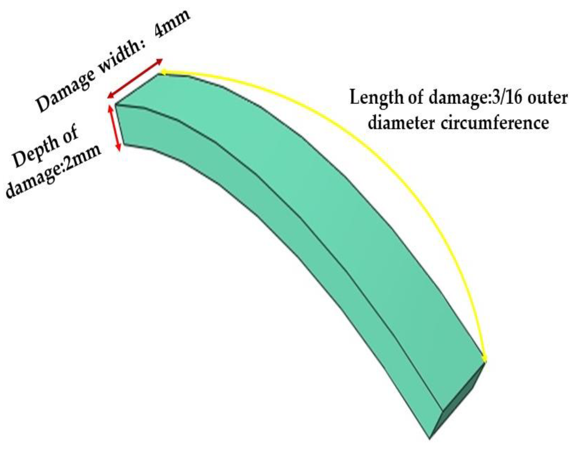
Applsci 13 08850 g002
Figure 3. Schematic diagram of circumferential defects.
Applsci 13 08850 g003
Figure 4. Schematic of double defects with the same circumferential position in the pipeline structure.
Applsci 13 08850 g004
Figure 5. Defect layout diagram for dual defects in pipeline structures at different circumferential positions.
Applsci 13 08850 g005
Figure 6. Two-dimensional damage index matrix for pipeline structures with dual defects at the same circumferential position 4. 4 The axial distance of damage in the figure is the distance between the second defect and the piezoelectric element sensor, with the first defect always located at a position 750 mm away from the piezoelectric element sensor. The axial distance between the second defect and the piezoelectric element sensor was set as 750 mm, such that the position of the first defect overlapped with that of the second defect, meaning that there was only one defect in the pipeline structure.
Applsci 13 08850 g006
Figure 7. Time-domain comparison plots for the operating conditions: (a) comparison of the piezoelectric time-domain signals between case 10 and case 11, (b) the partial detailed diagrams of case 10 and case 11, (c) comparison of the piezoelectric time-domain signals between case 10 and case 12, and (d) the partial detailed diagrams of case 10 and case 12.
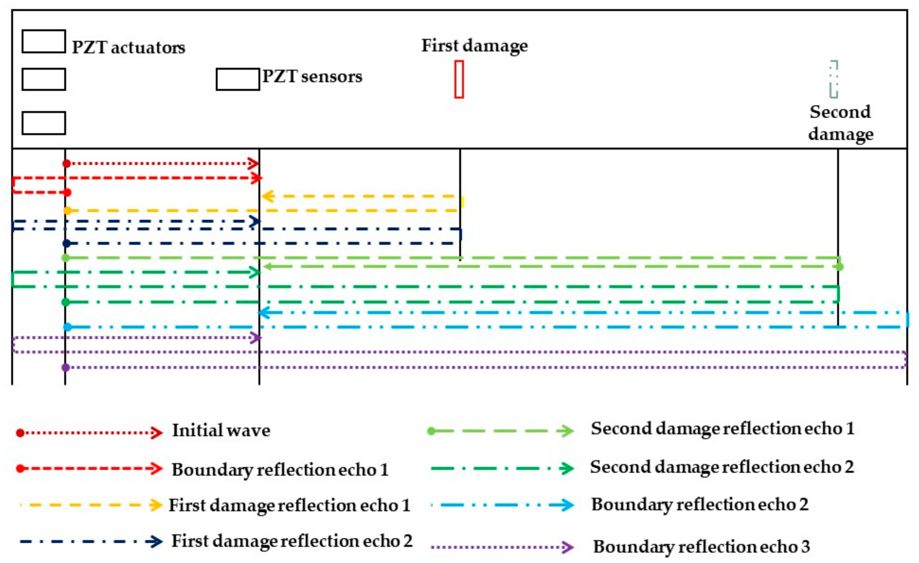
Applsci 13 08850 g007
Figure 8. The propagation mechanism of guided waves in pipeline structures with dual defects.
Applsci 13 08850 g008
Figure 9. Sensor signal diagram.
Applsci 13 08850 g009
Figure 10. The two-dimensional damage index matrix for dual defects in pipeline structures with different circumferential positions 6. 6 The axial distance of the damage shown in the figure refers to the distance between the second defect and the piezoelectric element sensor. The first damage is always located at 750 mm from the piezoelectric element sensor.
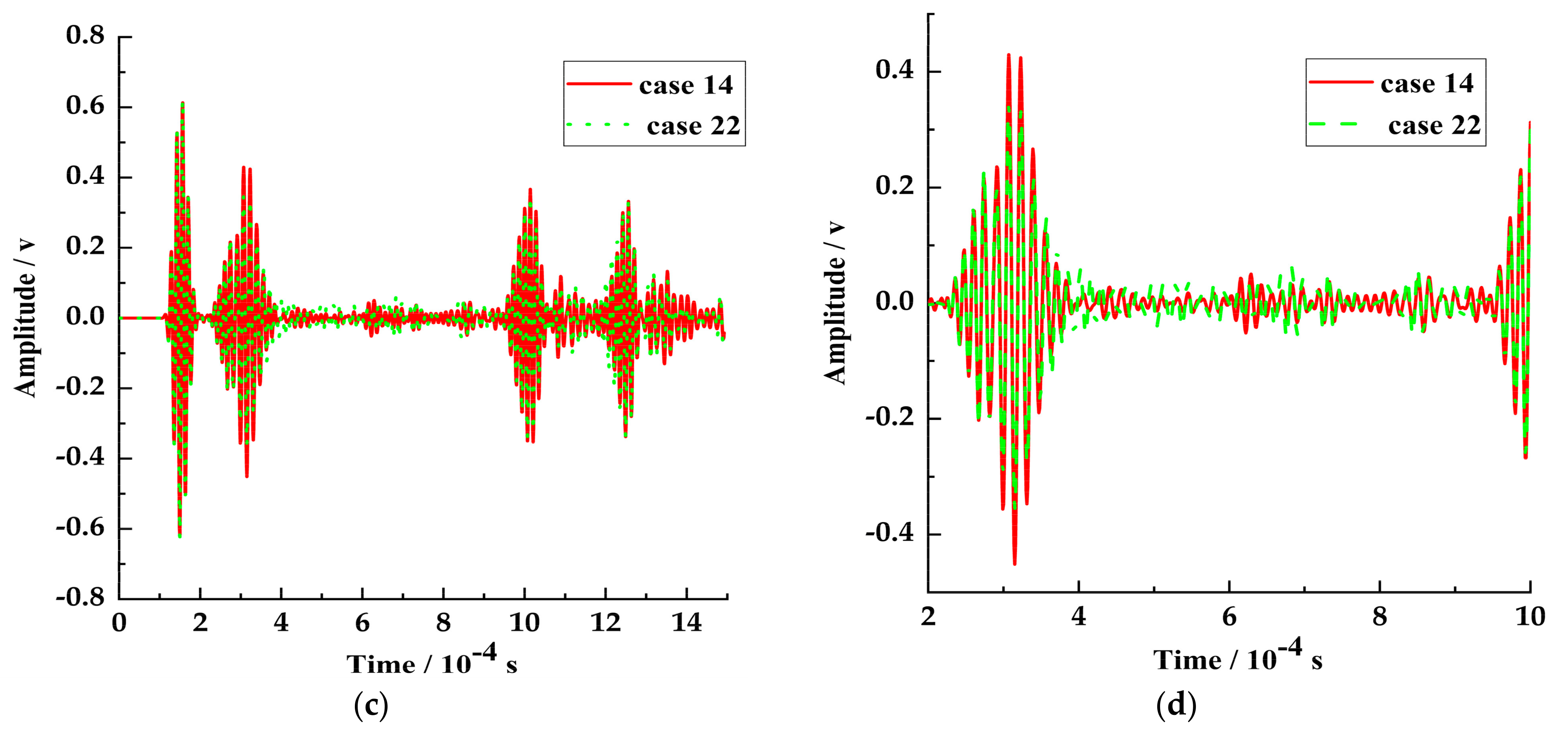
Applsci 13 08850 g010
Figure 11. Piezoelectric time domain comparison 7: (a) piezoelectric time domain diagram of case 14, (b) piezoelectric time domain diagram of case 22, (c) piezoelectric time domain comparison between case 14 and case 22, (d) piezoelectric temporal domain local amplification diagram. 7 For case 14 and case 22, the reflection echo 2 of the first defect, and the reflection echo 1 of the second defect propagated the same distance in the pipeline, so the two wave packets completely overlapped at this time.
Applsci 13 08850 g011aApplsci 13 08850 g011b
Figure 12. The comparison of the damage index matrices for pipeline structures 8. 8 The axial distance of the damage in the figure refers to the axial distance between the second defect and the piezoelectric element sensor. As the single-layered pipeline structure had only one defect, the axial distance of the damage refers to the axial distance between the damage and the piezoelectric element sensor.
Applsci 13 08850 g012
Figure 13. Radial schematic diagram of the layered pipeline structure.
Applsci 13 08850 g013
Figure 14. Experimental system for layered pipeline structures.
Applsci 13 08850 g014
Table 1. The pipeline structure material properties.
Type of
Structure
Internal Diameter/mmOuter Diameter/mmWall Thickness/mmDensity/kg·m−3Modulus of Elasticity/PaPoisson RatioTube Length/m
Material Properties
Steel tube6876478502.1 × 10110.322.7
Rigid polyurethane foam7613620807.8 × 1080.252.1
High-density polyethylene13614029465.52 × 1080.42.1
Table 2. Single defect model case for the pipeline structure 1.
CaseDamage Axial Distance/mm
case 10
case 2750
case 3900
case 41050
case 51200
case 61350
case 71500
case 81650
case 91800
1 The damage axial distance is the axial distance between the damage and the piezoelectric element sensor, where case 1 is a non-destructive pipe structure.
Table 3. Meshing of the finite element model 2.
Structure NameElement TypeGrid Size/mmNumber of Grids
piezoelectric elementC3D8E1220
structural layerC3D20R549,674
insulation layerC3D20R5107,520
anticorrosive layerC3D20R536,960
2 The insulation layer and anticorrosive layer in the subsequent analysis had different numbers of defects, compared to the number of grids presented in this table. However, the number of grids for other models remained the same. For the sake of simplicity, please refer to this table for the grid division of relevant models in the subsequent analysis.
Table 4. Operational parameters of the finite element model with the same circumferential position in pipeline structural health monitoring 3.
CaseFirst Defect Axial Distance/mmSecond Defect
Axial Distance/mm
Spacing of
Damage/mm
case 107507500
case 11750900150
case 127501050300
case 137501200450
case 147501350600
case 157501500750
case 167501650900
case 1775018001050
3 The axial distances of the first and second defects are both the axial distances between the defects and the piezoelectric transducer sensor. The first and second defects are located on the same generatrix.
Table 5. Finite element model operating conditions for different circumferential positions.
CaseFirst Defect Axial Distance/mmSecond Defect Axial Distance/mmSpacing of Damage/mmDouble Defect Relative Circumferential Position Change/°
case 18750750090
case 1975090015090
case 20750105030090
case 21750120045090
case 22750135060090
case 23750150075090
case 24750165090090
case 257501800105090
Table 6. Comparison of the times at which the piezoelectric element sensors received the wave packets 5.
Receiving Time/sRefection Echoes 1 of First Defect/sReflection Echoes 2 of First Defect /sRefection Echoes 1 of Second Defect/sReflection Echoes 2 of Second Defect/s
Case
case 104.07 × 10−46.37 × 10−44.07 × 10−46.37 × 10−4
case 114.07 × 10−46.37 × 10−44.65 × 10−47.14 × 10−4
case 124.07 × 10−46.37 × 10−45.22 × 10−47.72 × 10−4
5 The receiving time of the first reflection of the second defect for case 11, and the receiving time of the second reflection of the second defect for case 12, in Table 6, were the theoretically derived receiving times.
Table 7. The comparison between the finite element simulation, and the theoretical calculation, for the second defect.
CaseTime of Dissemination/sFinite Element Simulation Propagation Velocity/m·s−1The Second Defect Theoretical Damage Distance/mThe Second Defect Finite Element Simulation Damage Distance/mError/%
case 177.3 × 10−451911.81.8954
Table 8. Comparison of the damage index values for single and double defects, based on the damage index value.
PD/mmDescription of
Features
Reasons
750 P D 1500
1.7 λ P D 3.4 λ
I double   defect   0 ° > I signal   defect When   l 1.36 λ , overlap of reflection echoes and increase in pulse width. When   1.36 λ < l 1.70 λ , reflection echoes gradually separate from each other, but the mode conversion wave still overlaps with the reflection echoes.
1650 P D 1800
3.8 λ P D 4 λ
I double   defect   0 ° < I signal   defect On   the   one   hand ,   when   2.04 λ l , complete separation of reflection echoes.On the other hand, the reflection echoes of the damage have a longer propagation distance and lower waveform amplitude.
Table 9. Comparison of damage index values based on different circumferential positions.
Content of InfluencePD/mmPerformanceReasons
I value 750 P D 1800
1.7 λ P D 4 λ
I double   defect   0 ° > I double   defect   90 ° Changing the circumferential position caused a phase difference, which led to a decrease in the overall waveform amplitude.
The trend of I 750 P D 1350
1.7 λ P D 3 λ
I double   defect   0 ° was cyclical When   l 1.36 λ , the phase difference caused the reflection echoes to cancel out or reinforce each other.
I double   defect   90 ° showed a decreasing trend followed immediately by an increasing trendIn addition to an increase in l, the phase difference also played a role.
1350 P D 1500
3 λ P D 3.4 λ
I double   defect   0 °     and   I double   defect   90 °   both showed an increasing trendThe damage echo of the damage gradually separated, and the pulse width of the waveform increased.
1500 P D 1800
3.4 λ P D 4 λ
I double   defect   0 ° showed a slow downward trend At   this   point   l > 2.04 λ , the reflection echoes were completely separated, and the amplitude of the waveform decreased.
I double   defect   90 ° showed a rapid upward trendThe phase difference caused the overlap of the waveform between the reflection echoes of the defect and the boundary reflection echoes.
Table 10. Experimental conditions.
Condition NameFirst Defect Axial Distance/mmSecond Defect Axial Distance/mmSpacing of Damage/mmDouble Defect Relative Circumferential Position Change/°
case 50120000
case 80165000
case 1375012004500
case 1675016509000
case 21750120045090
case 24750165090090
Table 11. Comparison between the experimental and simulation results.
CaseSourceDamage Index ValueError/%
case 13Experiment0.393230.4
Finite element simulation0.39166
case 21Experiment0.258780.82
Finite element simulation0.26093
Table 12. Comparison of single and double damage based on experimental damage index values.
PD/mmCaseThe Number of Defects and Their Relative Circumferential PositionDamage Index ValueRelationship between the Magnitude of the Damage Index Value
1.7 λ P D 3.4 λ case 5Single defect0.32987 I double   defect   90 ° < I signal   defect < I double   defect   0 °
case 13Double defect 0°0.39323
case 21Double defect 90°0.25878
3.7 λ P D 4 λ case 8Single defect0.33861 I double   defect   90 ° < 0.3 < I double   defect   0 ° < I signal   defect
case 16Double defect 0°0.32174
case 24Double defect 90°0.25985
Disclaimer/Publisher’s Note: The statements, opinions and data contained in all publications are solely those of the individual author(s) and contributor(s) and not of MDPI and/or the editor(s). MDPI and/or the editor(s) disclaim responsibility for any injury to people or property resulting from any ideas, methods, instructions or products referred to in the content.

