Adaptive Optical Closed-Loop Control on the Basis of Hyperparametric Optimization of Convolutional Neural Networks

Abstract

In adaptive optics systems, the precision wavefront sensor determines the closed-loop correction effect. The accuracy of the wavefront sensor is severely reduced when light energy is weak, while the real-time performance of wavefront sensorless adaptive optics systems based on iterative algorithms is poor. The wavefront correction algorithm based on deep learning can directly obtain the aberration or correction voltage from the input image light intensity data with better real-time performance. Nevertheless, manually designing deep-learning models requires a multitude of repeated experiments to adjust many hyperparameters and increase the accuracy of the system. A wavefront sensorless system based on convolutional neural networks with automatic hyperparameter optimization was proposed to address the aforementioned issues, and networks known for their superior performance, such as ResNet and DenseNet, were constructed as constructed groups. The accuracy of the model was improved by over 26%, and there were fewer parameters in the proposed method, which was more accurate and efficient according to numerical simulations and experimental validation.

1. Introduction

Adaptive optics systems use control algorithms to correct for aberrations and measure phases in real time with a wavefront sensor to ensure the optical system is immune to interference and adaptable to the environment; therefore, they have been widely used in laser communications, femtosecond lasers, and astronomical observations [1,2,3,4,5,6,7]. Currently, Shack–Hartmann wavefront sensors are the most effective and popular wavefront sensors [8]. However, unfavorable conditions, such as a weak target light source, an uneven light intensity distribution, and a high large light amplitude, result in a threshold value that is too low for the wavefront to interpret an accurate, leading below which the wavefront sensor extracts the effective signal leads to a significant reduction in the measurement accuracy that affects the dynamic correction performance of adaptive optics [9,10]. In contrast, a wavefront sensorless system has a higher accuracy than systems with wavefront sensors when the target light energy is weak, and their simple construction makes adaptive optics more affordable than other solutions under certain circumstances [11].

In general, wavefront sensorless systems are divided into two main categories: model-based and model-free correction algorithms. Model-based optimal control algorithms include the mode method and the optical principle method [12,13,14]. Theoretically, model-based algorithms need to calculate and measure the relevant parameters of a complex system model, which is considerably complex. The two most common types of model-free correction algorithms are optimization algorithms and neural networks. The optimization algorithms predominantly include the stochastic parallel gradient descent algorithm (SPGD), the particle swarm optimization algorithm (PSO), and the simulated annealing algorithm. Such algorithms calculate the system evaluation function using the far-field light intensity data and iterate continuously until the evaluation function reaches the optimal point of the system, thereby achieving the wavefront correction [15,16]. However, the optimization algorithm requires multiple iterations. Furthermore, as the system dimension increases, the convergence speed slows, making it difficult to meet the high demands of real-time system performance at a high resolution system requirements. Nevertheless, the neural network class only needs to extract the image data once to complete the wavefront correction, which improves its real-time performance of the wavefront correction.

Fienup [17] proposed the adoption of the Inception v3 network to predict the phase information. The input of a CNN was the far-field image, and the output was the Zernike coefficient. This coefficient was employed to generate the phase information without iterations. R. Swansson et al. [18] changed the idea of the output Zernike coefficient and employed the U-Net network to directly predict the phase map of the wavefront. Lejia Hu et al. [19] ameliorated an SH-Net on the basis of ResNet and U-Net results. The inputs of the network were the data collected by the Hartmann sensor, and the output was the wavefront phase image. Yuan Xiuhua et al. adopted EfficientNet-B0 [20] to predict sixty-six Zernike coefficients [21]. Nevertheless, these algorithms still needed to calculate the correction voltage using a wavefront correction algorithm with the phase information. These networks, such as U-Net and Resnet, are excellent in the field of image classification. Rico Landman [22] proposed a method using reinforcement learning, which uses a model-free reinforcement learning algorithm to optimize the recurrent neural network controller, which could effectively learn the random disturbances caused by the telescope’s own vibration, hysteresis, and atmospheric disturbances, and it continuously adapted to the external environment. Using this method, the adaptive optical system has a strong ability to adapt to the environment and enhance the correction accuracy, which increased its application potential, but this method did not consider the impact of the network model’s size on the correction accuracy. Therefore, this study focused on the automatic selection of a suitably size network to improve the accuracy of the neural network model.

Qinghua Tian [23] investigated the effects of the size of a convolutional neural network on the prediction accuracy of the Zernike coefficient prediction accuracy. When the convolutional neural network model was too small, the network was poorly fitted; when the model was too large, the performance degraded due to over-fitting and gradient disappearance. The manual design of high-precision convolutional neural networks requires professional experience to adjust the network’s hyperparameters multiple times [24,25]. Therefore, this method required a great deal of computational and human resources to increase the network’s accuracy and could not guarantee improvements in the network’s accuracy and efficiency [26,27,28]. To resolve the above problems, an adaptive optical closed-loop control algorithm, based on the hyperparametric optimization of convolutional neural networks, was proposed.

In this paper, a set of hyperparameter optimization frameworks was designed that prioritized the automation of the model design and its accuracy, resulting in a model (Auto-U-net) with higher prediction accuracy. In addition, the model (Auto-U-net) directly predicted and controlled the correction voltage values without calculating additional data calculations. The manually designed convolutional neural networks, such as ResNet and DenseNet, were built as the convolutional neural network contrast groups. The hyperparameter optimization strategy was first applied to adaptive optics. Subsequently, a set of appropriate hyperparameter convolutional neural networks was automatically selected. Moreover, the convolutional neural network model (U-net) with the optimal accuracy and minimal parameters was iterated in order to improve the accuracy and efficiency of adaptive optics systems.

2. Fundamental Principles

2.1. Principles and Methods of Wavefront Sensorless Control Systems in the Basis of Convolutional Neural Networks

A neural network is an algorithm that resembles the biological brain process and has an effective non-linear fitting capability to represent the functional relationship between input and output information. Convolutional neural networks are frequently employed in the field of imaging [29] and are well suited for use in wavefront sensorless adaptive optics systems. In large-scale image feature extraction tasks, they have had significant success. In this paper, the SPGD algorithm was used to correct the random aberrations, and the corrected voltage values were used as true values for the training of the convolutional neural network.

2.2. Principles of Hyper-Parameter Optimization Convolutional Neural Network

The hyperparameters of a convolutional neural network consist of the number of layers, the width of each layer, the size of the convolutional kernel, the step-size of the convolutional layers, the use of inflation convolution to expand the field of perception, the inflation rate of the null convolution, the dropout-layer rounding rate, the type of pooling layer, the type of activation function, the number of fully connected layer neurons, the learning rate, the type of optimization, and other parameters.

These hyperparameter optimization challenges typically involve non-convex, noisy and other complex characteristics, and the optimal set of hyperparameters cannot be obtained by the conventional gradient descent method, and it is very time-consuming to find an accuracy-optimal model by traversing all hyperparameters. A random search is more efficient than traversal method, but it still requires a multitude of samples for multiple iterations. The black-box function is constructed, and the optimal function value is iterated through its posterior probability. The principle of the Bayesian optimization CNN network is to use the hyperparameters of CNN and the loss function value of the CNN testing dataset corresponding to the hyperparameters as data to build a probabilistic surrogate model, and calculate the optimized hyperparameters through the acquisition function. When the Bayesian optimization was completed, a neural network model with high accuracy and strong generalization ability was obtained.

The Bayesian optimization was performed, as follows:

The variable $f\left(x\right)$ is the mapping from the hyperparameter x to the model function, where $x\in X,X\subseteq R^d,X$ is the hyperparameter of the n dimensional system, and the goal of hyperparameter optimization was to find the optimal value of the model function within the hyperparameter set and record the n-dimensional system hyperparameters $x^{*}$, corresponding to the optimal value. Consider the maximum value:

$$x^{*}=argmaxf\left(x\right),$$

(1)

where $f\left(x\right)$ is a black-box function. For instance, the known data are $Dat{a}_{1:t}=(x_i,y_i),i=1,2,\cdots ,t,$ where $y_i$ is the accuracy under the test set of the model trained by hyperparameter $x_i$ , and the current evaluated data are denoted as $Data$. This could estimate the optimal value of the black-box function in a small known small data set. In the following sections, the probabilistic surrogate model was adopted to fit the black-box function. Aside from that, the optimal value of the black-box function was iterated by the acquisition function in accordance with the known $Data$.

A probabilistic surrogate model was employed to fit the objective function of the black-box function. Moreover, the resulting testing dataset y was regarded as a random observation of the black-box function, and then $y=f\left(x\right)+\epsilon$, where the noise $\epsilon$ satisfied the Gaussian (normal) distribution $p\left(\epsilon \right)=N(0,{\sigma }_{\epsilon }^2)$. Starting from the prior of the black-box function, the probabilistic surrogate model optimized the black-box function model by continuously heightening the data information. The more data information obtained, the higher the fitting degree of the black-box function became [30]. Therefore, Gaussian processes were the paramount choice for model proxies. Apart from that, each subset of the Gaussian model exhibited a normal distribution. Assuming that the expectation of the objective function model was zero, the probability distribution of the new observation $(x_{t+1},y_{t+1})$ given the known data, was, as follows:

$$\left[y_t+1\right]\sim N(0,\left[\begin{array}{cc}\mathrm{K}+{\sigma }_{\epsilon }^{2}I& k\\ k^T& k(x_{t+1},x_{t+1})\end{array}\right]),$$

(2)

where: k : $x\ast x$ is the covariance function, $k={\left[k(x_1,x_{t+1}),\cdots ,k(x_t,x_{t+1})\right]}^{\mathrm{T}}$, and $\mathrm{K}$ in Equation (2) was, as follows:

$$\mathrm{K}=\left[\begin{array}{ccc}k(x_1,x_1)& \cdots & k(x_1,x_t)\\ ⋮& \ddots & ⋮\\ k(x_t,x_1)& \cdots & k(x_t,x_t)\end{array}\right],$$

(3)

where I is the identity matrix, and ${\sigma }_{\epsilon }^2$ is the noise variance. Considering both the original observation data and the new value of x to make the prediction, the posterior distribution of $y_{t+1}$ was, as follows: $P\left(y_{t+1}\left|y_{1:t},x_{1:t+1}\right.\right)=N({\mu }_t\left(x_{x+1}\right),{\sigma }_t^2\left(x_{t+1}\right))$.

The mathematical expectation and variance of $y_{t+1}$ was obtained, as follows:

$${\mu }_t\left(x_{t+1}\right)=k^T{(K+{\sigma }_{\epsilon }^{2}I)}^{-1}{y}_{1:t},$$

(4)

$${\sigma }_{t+1}=k(x_{t+1},x_{t+1})-k^T(K+{\sigma }_{\epsilon }^{2}I)k.$$

(5)

Gaussian regression usually adopts the Automatic Relevance Determination (ARD) squared exponential function with the formula:

$$K_{SE}(x,x^{\prime })={\theta }_{0}exp\left\{-\frac{1}{2}{r}^2(x,x^{\prime })\right\},$$

(6)

$$r^2(x,x^{\prime })=\sum _{d=1}^D{{\theta }_d(x_d-x_d^{\prime })}^2,$$

(7)

In Equations (6) and (7), ${\theta }_0$ is the length factor, the data D is bounded and ${\theta }_d$ is the covariance amplitude.

As a gather function, in a Bayesian optimization, the acquisition function a is employed to calculate the next evaluation point.

The acquisition function consists of the posterior probability distribution of the known data and selects the optimal value, which was employed as the next evaluation point:

$$x_{t+1}=argmax{a}_t(x;Data).$$

(8)

The acquisition functions were predominantly categorized as three types—a probability lifting function, an expectation lifting function, and a confidence upper-bound function [31]. The probability lifting function repalcedwas is employed here. The probability lifting function is defined as the probability that the new sample point has been improved relative to the optimal value of the black-box function. Assuming that $x^{+}$ was the optimal value of the black-box function, the hyper-parameters with enhanced values were obtained were obtained by sampling the following function:

$$a_{PI}\left(x\right)=P(f\left(x\right)\ge (f\left(x^{+}\right)-e))=\varphi \left(\frac{f(x^{+}-e-\mu \left(x\right))}{\sigma \left(x\right)}\right).$$

(9)

The Bayesian optimization algorithmic program flow diagram are shown in Figure 1, where T is the upper limit of the number of evaluation settings.

3. Analysis and Discussion

3.1. Numerical Simulation

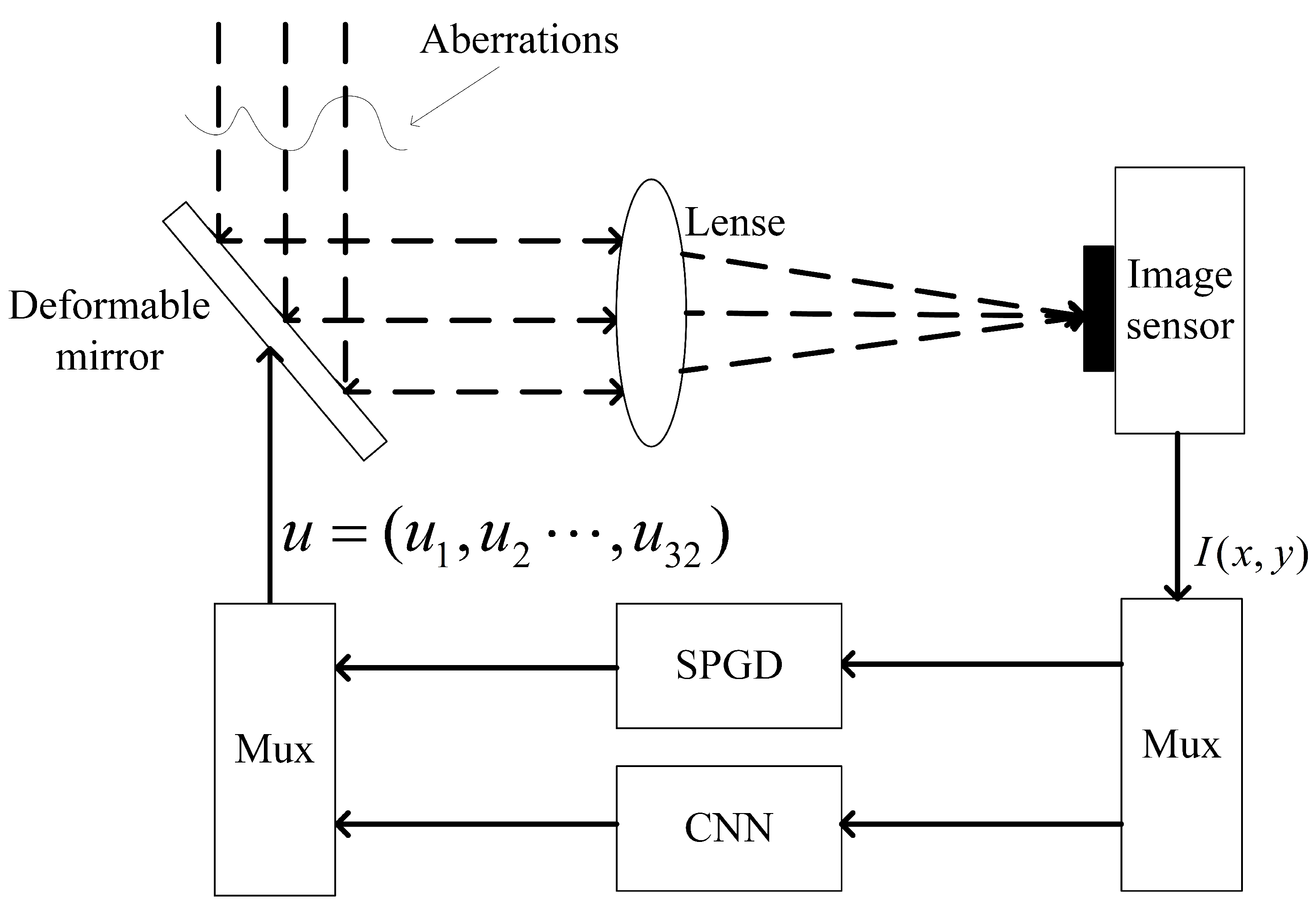
The numerical simulation control block diagram was shown in Figure 2. The voltage data were predicted directly using the CNN algorithm. To further improve the correction accuracy, the correction using the CNN algorithm was followed by a further correction using the SPGD algorithm. The CNN algorithm was used for coarse correction and the SGPD algorithm for fine correction.

The optimal set of hyperparameters was automatically chosen as the parameters of the convolutional neural network to minimize the loss value of the neural network testing dataset, including the optimal accuracy of the wavefront sensorless system based on the convolutional neural network with a Bayesian-based hyperparameter optimization model that used the testing set accuracy (root-mean-square error (RMSE)) of the convolutional neural network as the optimization target. In practice, the amount of hyperparameter regulation increased exponentially as a result of the excessive number of network layers. As a result, by stacking the same network blocks, the hyperparameters of each network layer were shared, and the amount of hyperparameter conditioning was decreased.

Table 1. Hyperparameter types and their selection ranges.

Hyperparameters	Value Range of the Hyperparameters (Integer, Floating Point, Boolean, and Character)
Number of network stacking layers	3–12
Network width of each layer	4–40
Convolution kernel size	1–7
Convolution step size	1–3
Fill or not	0 or 1
Pooling mode	Max Pooling, verage Pooling, Mix Pooling, Stochastic Pooling
Activation function type	Sigmoid, Tanh, ReLu, Leaky, ReLu, ELU
The number of neurons in the adequately connected layer	256–1024
Type of optimization algorithm	Adam, Sgd
Optimized the learning rate of the algorithm	0.0001–0.01

displays the hyperparameter selection range.

The control group models included ResNet, DenseNet, etc. ResNet introduced residual blocks to address the gradient disappearance issue created by a high number of network layers, enabling layer stacking to increase the network accuracy. DenseNet built on ResNet’s foundation by having a stronger generalization capability while maintaining Resnet’s accuracy. Regularization and other aspects were improved in Inception v3, which lessened the problem of model over-fitting; using a minimal amount of data, U-Net excels at image segmentation. Inception v3 had enhanced regularization to lessen model over-fitting. U-Net has made significant progress in image segmentation, achieving excellent segmentation outcomes with modest datasets. Moreover, the concept behind EfficientNet-B0 was to create a standard convolutional network extension model in order to increase accuracy while using less computational power.

3.2. Numerical Analysis and Discussion

In the numerical simulation, 5000 sets of random aberrations were generated, and the corrected voltage values were obtained by correcting the aberrations with the SGPD algorithm, and the voltage values were used as true values for the training of the neural network. To simulate real experiments, random noise was added. From these 5000 sets, 4000 sets served as the convolutional neural network’s training data, and the remaining 1000 sets served as the network’s testing data. The neural network was fed 128*128 pixel far-field spots and outputs 32-unit correction voltage values.

The hyperparameters of the U-net network were set, as follows: The number of convolutional network layers was 22, the width was 64, the convolutional kernel size was 3, the convolutional step-size was 1, there was no padding, the pooling method was Max Pooling, the activation function was RuLe, the number of fully connected neurons was 638,976 , the optimization algorithm was Adam, and the learning rate was the default.

Compared with SPGD algorithm, the correction time of SPGD algorithm was 3.18 ms, while the neural network in this paper only needed 0.32 ms. Since the training data of the neural network was obtained from SPGD algorithm, the accuracy was not as high as SPGD algorithm. However, the correction accuracy and speed can be greatly improved by the method of coarse correction of neural network and fine correction of SPGD.

Table 2. Model types and their performances.

Types of Models	Test Set Optimal RMSE (V)	Number of Model Parameters
Auto-U-net	0.5476 V	5,946,094
Resnet18	3.1584 V	58,430,240
Inception v3	1.1312 V	21,249,511
U-net	0.898 V	40,492,546
EfficientNet-B0	1.2569 V	7,247,472
DenseNet	1.864 V	12,687,072

compares the performance of this paper’s network Auto-U-net to that of a manually designed convolutional neural network (i.e., ResNet18, Inception v3, U-Net, EfficientNet-B0, and DenseNet). This illustrated the hyperparametrically optimized convolutional neural network performed significantly better in terms of the testing set and used fewer model parameters. As compared to the accuracy to the U-Net network, a 26 percent improvement was observed. A total of three convolutional network layers, a width of 32, three convolutional kernels, one convolutional step, no padding, Max Pooling as the pooling method, Tanh as the activation function type, 25,646 as the number of fully connected layer neurons, Adam as the optimization algorithm type, and 0.0045 as the learning rate were the optimized hyperparameters.

Figure 3 illustrates the comparison between the predicted value of the convolutional neural network after the hyperparameter optimization and the truevalue. Table 2 shows the RMSE values and the number of network parameters for the manually designed network and the network optimized by hyperparameters. It can be seen that the overall prediction effect was improved.

3.3. Experimental and Result Analysis

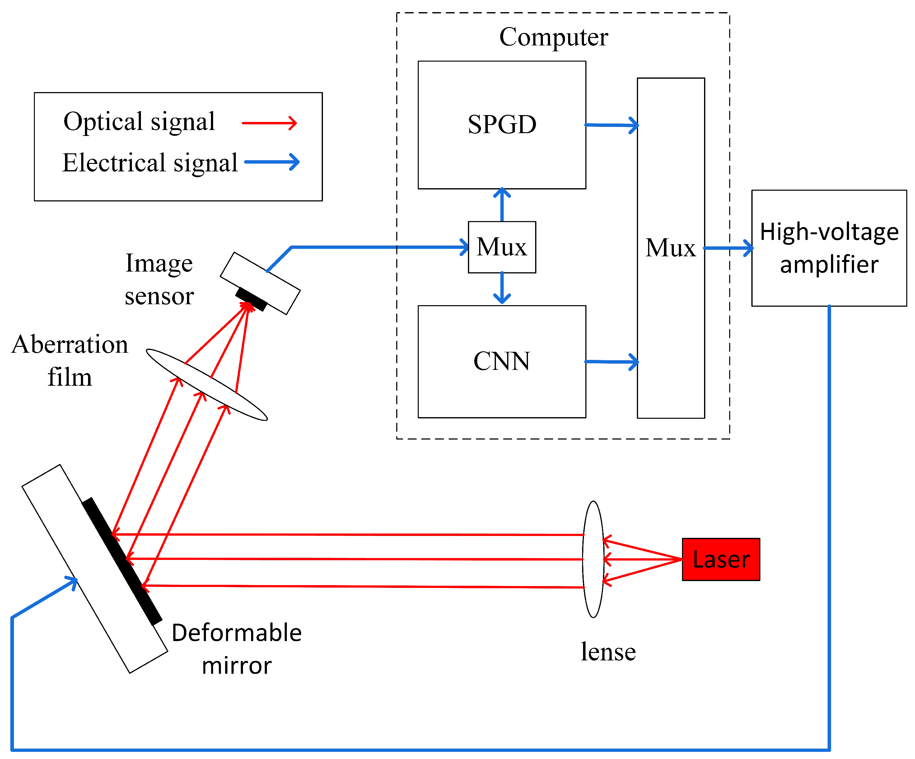
As depicted in Figure 4, to test the effectiveness of the algorithm, a wavefront sensorless adaptive optics experimental system, based on a hyperparametric convolutional neural network, was created. First, 39 unit voltage data were obtained by SPGD algorithm to correct for random aberrations, where 0–27 V was represented by the numerical value of 0–4000 scaled Volt(sV), whose random data mean is 2000 scaled Volt(sV). Next, the corresponding far-field spot data and voltage data were obtained from the image sensor and stored as the training and testing datasets of the convolutional neural network, which received 128*128 pixel far-field spot data as input and produced 39 voltage data as output. The testing dataset size was 1000, the training dataset size was 4000, and the hyperparameter optimization range was consistent with the information provided above.

The optimized hyperparameters were as follows. The width of the convolutional network was 40, the number of convolutional layers was 9, the convolutional kernel size was 3, the convolutional step-size was 1, the pooling method is Max Pooling, the activation function type was tanh, the number of fully connected layer neurons was 3185, the optimization algorithm type was Adam, and the learning rate was 0.0063.

Figure 5 shows the testing dataset comparison between the hyperparameter-optimized convolutional neural network Auto-U-net and the artificially designed convolutional neural network U-Net. As revealed by the above analysis, the testing set accuracy of the optimized network was significantly higher than that of the U-net network. Moreover, the root-mean-square-error (RMSE) of the predicted voltage of the algorithm in this paper was 41,246. The RMSE of the U-net network predicted voltage was 55,546, and the accuracy was increased by more than 26%. It demonstrated that the hyperparameter-optimized convolutional network outperformed the manually designed convolutional neural network in terms of accuracy.

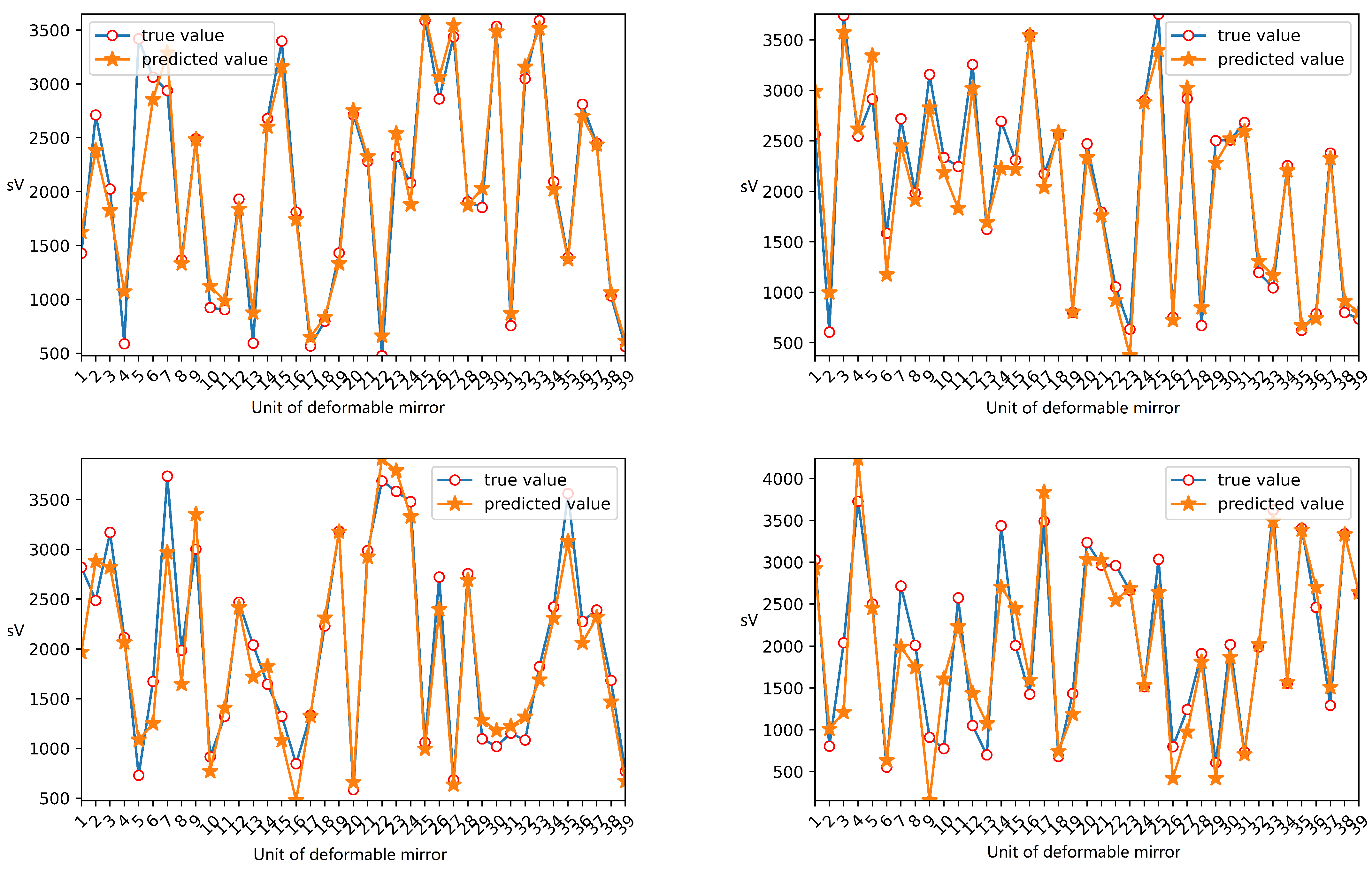
Figure 6 shows the comparison between the predicted value of 39 units of the deformable mirror as predicted by the hyperparameter- optimized convolutional neural network and the truevalue. The data on the horizontal axis represented the number of units of the deformable mirror, and the vertical axis represented the true value and predicted value of each unit of the deformable mirror. The overall prediction performance was good, and the error between the true value and predicted value of each unit of the deformable mirror was small. It showed that the model in this paper could accurately extract features from random distortion images and obtain random distortion correction data. The experiment in this paper was carried out on an GTX1070 graphics card, and it took approximately 0.32 ms to execute the model trained in this paper, and the frequency reached 3 kHZ.

4. Conclusions

In this paper, a wavefront sensorless system was developed using hyperparametric optimization of a convolutional neural network to automate their design for use in adaptive optics. The simulation and field experiments confirmed that the hyperparametric-based convolutional neural networks had a higher prediction accuracy than the conventional, manually designed convolutional neural networks, with a 30% improvement in accuracy, as compared to the U-net, and fewer model parameters. In addition, it was demonstrated that the convolutional neural network could predict the correction voltage directly, as compared to the traditional wavefront sensorless control algorithm, and the correction voltage only needed to be calculated one time, which significantly improved the real-time, dynamic performance and control accuracy of an adaptive optics system. To realize the miniaturization and low cost of the a wavefront sensorless system, additional research must be conducted on related topics, such as the construction of high-precision lightweight convolutional neural networks.

References

1. Nishizaki, Y.; Valdivia, M.; Horisaki, R.; Kitaguchi, K.; Saito, M.; Tanida, J.; Vera, E. Deep learning wavefront sensing. Opt. Express 2019, 27, 240–251. [Google Scholar] [CrossRef] [PubMed]
2. Toselli, I.; Gladysz, S. Improving system performance by using adaptive optics and aperture averaging for laser communications in oceanic turbulence. Opt. Express 2020, 28, 17347–17361. [Google Scholar] [CrossRef]
3. Sun, L.; Guo, Y.; Shao, C.; Li, Y.; Zheng, Y.; Sun, C.; Wang, X.; Huang, L. 10.8 kW, 2.6 times diffraction limited laser based on a continuous wave Nd: YAG oscillator and an extra-cavity adaptive optics system. Opt. Lett. 2018, 43, 4160–4163. [Google Scholar] [CrossRef] [PubMed]
4. Pomohaci, R.; Oudmaijer, R.D.; Goodwin, S.P. A pilot survey of the binarity of Massive Young Stellar Objects with K-band adaptive optics. Mon. Not. R. Astron. Soc. 2019, 484, 226–238. [Google Scholar] [CrossRef] [Green Version]
5. Azimipour, M.; Migacz, J.V.; Zawadzki, R.J.; Werner, J.S.; Jonnal, R.S. Functional retinal imaging using adaptive optics swept-source OCT at 1.6 MHz. Optica 2019, 6, 300–303. [Google Scholar] [CrossRef] [PubMed]
6. Salter, P.S.; Booth, M.J. Adaptive optics in laser processing. Light Sci. Appl. 2019, 8, 1–16. [Google Scholar] [CrossRef] [Green Version]
7. Chen, J.; Ma, J.; Mao, Y.; Liu, Y.; Li, B.; Chu, J. Experimental evaluation of a positive-voltage-driven unimorph deformable mirror for astronomical applications. Opt. Eng. 2015, 54, 117103. [Google Scholar] [CrossRef]
8. Zhao, F.; Huang, W.; Xu, W.; Yang, T. Optimization method for the centroid sensing of Shack-Hartmann wavefront sensor. Infrared Laser Eng. 2014, 43, 3005–3009. [Google Scholar]
9. Barchers, J.; Fried, D.; Link, D. Evaluation of the performance of Hartmann sensors in strong scintillation. Appl. Opt. 2002, 41, 1012–1021. [Google Scholar] [CrossRef]
10. Wei, P.; Li, X.; Luo, X. Influence of lack of light in partial subapertures on wavefront reconstruction for shack-Hartmann wavefront sensor. Chin. J. Lasers 2020, 47, 0409002. [Google Scholar]
11. Wu, Z.; Zhang, T.; Mbemba, D.; Wang, Y.; Wei, X.; Zhang, Z.; Iqbal, A. Wavefront Sensorless Aberration Correction with Magnetic Fluid Deformable Mirror for Laser Focus Control in Optical Tweezer System. IEEE Trans. Magn. 2020, 57, 4600106. [Google Scholar] [CrossRef]
12. Booth, M.J. Wavefront sensorless adaptive optics for large aberrations. Opt. Lett. 2007, 32, 5–7. [Google Scholar] [CrossRef]
13. Huang, L.H. Coherent beam combination using a general model-based method. Chin. Phys. Lett. 2014, 31, 094205. [Google Scholar] [CrossRef]
14. Liu, M.; Dong, B. Efficient wavefront sensorless adaptive optics based on large dynamic crosstalk-free holographic modal wavefront sensing. Opt. Express 2022, 30, 9088–9102. [Google Scholar] [CrossRef]
15. Yang, H.; Li, X. Comparison of several stochastic parallel optimization algorithms for adaptive optics system without a wavefront sensor. Opt. Laser Technol. 2011, 43, 630–635. [Google Scholar] [CrossRef]
16. Ren, H.; Dong, B. Fast dynamic correction algorithm for model-based wavefront sensorless adaptive optics in extended objects imaging. Opt. Express 2021, 29, 27951–27960. [Google Scholar] [CrossRef]
17. Paine, S.W.; Fienup, J.R. Machine learning for improved image-based wavefront sensing. Opt. Lett. 2018, 43, 1235–1238. [Google Scholar] [CrossRef] [Green Version]
18. Swanson, R.; Lamb, M.; Correia, C.; Sivanandam, S.; Kutulakos, K. Wavefront reconstruction and prediction with convolutional neural networks. In Proceedings of the Adaptive Optics Systems VI; SPIE: Austin, TX, USA, 2018; Volume 10703, pp. 481–490. [Google Scholar]
19. Hu, L.; Hu, S.; Gong, W.; Si, K. Deep learning assisted Shack–Hartmann wavefront sensor for direct wavefront detection. Opt. Lett. 2020, 45, 3741–3744. [Google Scholar] [CrossRef]
20. Tan, M.; Le, Q. Efficientnet: Rethinking model scaling for convolutional neural networks. In Proceedings of the International Conference on Machine Learning, PMLR, Beach, CA, USA, 10–15 June 2019; pp. 6105–6114. [Google Scholar]
21. Wang, M.; Guo, W.; Yuan, X. Single-shot wavefront sensing with deep neural networks for free-space optical communications. Opt. Express 2021, 29, 3465–3478. [Google Scholar] [CrossRef]
22. Landman, R.; Haffert, S.Y.; Radhakrishnan, V.M.; Keller, C.U. Self-optimizing adaptive optics control with reinforcement learning for high-contrast imaging. J. Astron. Telesc. Instruments Syst. 2021, 7, 039002. [Google Scholar] [CrossRef]
23. Tian, Q.; Lu, C.; Liu, B.; Zhu, L.; Pan, X.; Zhang, Q.; Yang, L.; Tian, F.; Xin, X. DNN-based aberration correction in a wavefront sensorless adaptive optics system. Opt. Express 2019, 27, 10765–10776. [Google Scholar] [CrossRef] [PubMed]
24. Masum, M.; Shahriar, H.; Haddad, H.; Faruk, M.J.H.; Valero, M.; Khan, M.A.; Rahman, M.A.; Adnan, M.I.; Cuzzocrea, A.; Wu, F. Bayesian hyperparameter optimization for deep neural network-based network intrusion detection. In Proceedings of the 2021 IEEE International Conference on Big Data (Big Data), Orlando, FL, USA, 15–18 December 2021; pp. 5413–5419. [Google Scholar]
25. Chalasani, S.R.; Selvam, G.T.; Chellaiah, C.; Srinivasan, A. Optimized convolutional neural network-based multigas detection using fiber optic sensor. Opt. Eng. 2021, 60, 127108. [Google Scholar]
26. Feurer, M.; Hutter, F. Hyperparameter optimization. In Automated Machine Learning; Springer: Cham, Switzerland, 2019; pp. 3–33. [Google Scholar]
27. Victoria, A.H.; Maragatham, G. Automatic tuning of hyperparameters using Bayesian optimization. Evol. Syst. 2021, 12, 217–223. [Google Scholar] [CrossRef]
28. Yang, L.; Shami, A. On hyperparameter optimization of machine learning algorithms: Theory and practice. Neurocomputing 2020, 415, 295–316. [Google Scholar] [CrossRef]
29. Yang, N.; Nan, L.; Zhang, D.; Ku, T. Research on image interpretation based on deep learning. Infrared Laser Eng. 2018, 47, 203002–0203002. [Google Scholar] [CrossRef]
30. Neiswanger, W.; Wang, K.A.; Ermon, S. Bayesian algorithm execution: Estimating computable properties of black-box functions using mutual information. In Proceedings of the International Conference on Machine Learning, PMLR, Virtual Event, 18–24 July 2021; pp. 8005–8015. [Google Scholar]
31. Ellinger, J.; Beck, L.; Benker, M.; Hartl, R.; Zaeh, M.F. Automation of Experimental Modal Analysis Using Bayesian Optimization. Appl. Sci. 2023, 13, 949. [Google Scholar] [CrossRef]
Figure 1. Bayesian optimization algorithmic program flow diagram.
Applsci 13 08589 g001
Figure 2. The numerical simulation control block diagram. The CNN algorithm was used for coarse correction and the SGPD algorithm was used for fine correction.
Applsci 13 08589 g002
Figure 3. The proposed algorithm predicted four groups of 32-unit voltage data in the numerical simulation.
Applsci 13 08589 g003
Figure 4. Adaptive optics system verification platform. When the aberration is small, the SPGD algorithm is selected; in other cases, the CNN algorithm is selected.
Applsci 13 08589 g004
Figure 5. Test set performance of Auto-U-net and U-net.
Applsci 13 08589 g005
Figure 6. The proposed algorithm predicts four groups of 39 unit voltage data in an experiment.
Applsci 13 08589 g006