Article

Anomalies in Infrared Outgoing Longwave Radiation Data before the Yangbi Ms6.4 and Luding Ms6.8 Earthquakes Based on Time Series Forecasting Models

Institute of Earthquake Forecasting, CEA, Beijing 100036, China
*
Author to whom correspondence should be addressed.
Appl. Sci. 2023, 13(15), 8572; https://doi.org/10.3390/app13158572
Submission received: 15 May 2023 / Revised: 21 July 2023 / Accepted: 22 July 2023 / Published: 25 July 2023
(This article belongs to the Special Issue Machine Learning Applications in Seismology)

Abstract

:
Numerous scholars have used traditional thermal anomaly extraction methods and time series prediction models to study seismic anomalies based on longwave infrared radiation data. This paper selected bidirectional long short-term memory (BILSTM) as the research algorithm after analyzing and comparing the prediction performance of five time series prediction models. Based on the outgoing longwave radiation (OLR) data, the time series prediction model was used to predict the infrared longwave radiation values in the spatial area of 5° × 5° at the epicenter for 30 days before the earthquake. The confidence interval was used as the evaluation criterion to extract anomalies. The examples of earthquakes selected for study were the Yangbi Ms6.4-magnitude earthquake in Yunnan on 21 May 2021 and the Luding Ms6.8-magnitude earthquake in Sichuan on 5 September 2022. The results showed that the observed values of the Yangbi earthquake 15 to 16 days before the earthquake (5 May to 6 May) exceeded the prediction confidence interval over a wide area and to a large extent. This indicates a strong and concentrated OLR anomaly before the Yangbi earthquake. The observations at 27 days (9 August), 18 days (18 August), and 8 days (28 August) before the Luding earthquake exceeded the prediction confidence interval in a local area and by a large extent, indicating a strong and scattered OLR anomaly before the Luding earthquake. Overall, the method used in this paper extracts anomalies in both spatial and temporal dimensions and is an effective method for extracting infrared longwave radiation anomalies.

1. Introduction

Since the 1980s, when the Soviet scientist Gornyy [1] first discovered anomalies in thermal infrared remote sensing images before earthquakes in Central Asia, researchers in various countries have been using thermal infrared data to study seismic activity and to attempt to predict earthquakes. Many scholars have used various methods to study pre-earthquake anomalies based on outgoing longwave radiation data, including wavelet variation methods [2], the robust satellite techniques (RST) algorithm [3], and the eddy field method [4], and to analyze pre-earthquake precursor patterns based on the spatial and temporal evolution of the anomalies. Time series studies of longwave radiation data could also demonstrate pre-earthquake anomalies from a single time dimension. Many scholars have used various methods to study changes in temporal OLR values, such as the geometric moving average martingale (GMAM) change detection method used by Kong et al. [5], the background field difference method and the mean value method used by Mahmood et al. [6], and the flux method used by Natarajan et al. [7], after processing the OLR data and displaying them on a two-dimensional image with time as the horizontal coordinate. The images showed anomalies that exceeded the thresholds. Many studies have shown that some thermal infrared anomalies may exist before earthquakes. However, some scientists have argued against this. For example, Prakash et al. [8] found no significant thermal anomalies before earthquakes in and around India after studying earthquakes in the region. Although there is no consensus on the mechanism of pre-earthquake infrared anomalies, it is generally accepted that a certain range of thermal anomalies can occur at some time before an earthquake. Significantly, Chinese seismologists introduced their research results of seismic infrared remote sensing into daily earthquake forecasting practice and obtained a good correspondence in the prediction of earthquake risk areas in 2008, 2009, and 2013 [9].
The Earth’s outgoing longwave radiation is the primary driver of the Earth’s climate. This energy’s reflection, absorption, and emission occur through a complex system of clouds, aerosols, atmospheric constituents, oceans, and land surfaces [10]. By definition, longwave radiation is the energy density of electromagnetic waves of all wavelengths radiated into outer space by the Earth’s atmospheric system. It can reflect the energy radiation of the Earth’s atmospheric system [11]. The outgoing longwave radiation data used were acquired by the High-Resolution Infrared Radiation Sounder (HIRS) carried by the National Oceanic and Atmospheric Administration’s (NOAA) polar-orbiting weather satellites. The NOAA satellite series has been continuously collecting longwave radiation data since the 1970s. These data have been used in a variety of applications due to the long accumulation of data and open-source access.
The rapid development of society has led to the generation of vast amounts of time series data in economics, meteorology, geology, and the environment. The correct application of time series data and forecasting models has been of great value to social activities. Classical time series forecasting models mainly include autoregressive moving average (ARMA) and autoregressive integrated moving average (ARIMA) models. Machine learning has a regression function that has been adapted to the characteristics of time series data. Various machine learning-based forecasting methods have been applied to time series data, including support vector machines, Bayesian networks, and Gaussian processes. With the development of deep learning, convolutional neural networks based on time series data, long short-term memory models, and multi-model hybrid models have been widely used and have achieved excellent performance [12]. Large amounts of data are required for data training of time series prediction models. The early deployment of seismic monitoring equipment and advances in observational monitoring techniques have facilitated the development of multiple types and long-time series of seismic data. These have provided favorable conditions for the application of time series forecasting models in the field of seismology. Saqib et al. [13,14] used the ARIMA algorithm for the short-term prediction of total electron content (TEC) and detected several pre-earthquake anomalies. In another paper published in the same year, the authors reported a better performance of the long short-term memory (LSTM) model than the ARIMA model in detecting seismic ionospheric anomalies. Some researchers have made improvements to the LSTM algorithm. A multi-network-based hybrid long and short-term memory (N-LSTM) model was proposed by Senturk et al. [15]; Yue et al. [16] combined the LSTM model and the relative power spectrum method for TEC anomaly detection; Xiong et al. [17] proposed an encoder–decoder extended short-term memory expansion model; all these improved models obtained better performance in their article applications.
In radon time series studies, Mohammed et al. [18] used the ARIMA model and Monte Carlo prediction model to find a good correlation between soil radon and micro-seismicity in the study area; Mir et al. [19] used different sets of algorithms to predict time series and detect anomalies for real-time soil radon time series of different scenarios; Feng et al. [20] studied groundwater radon and used an empirical mode decomposition–long short-term memory (EMD–LSTM) model to find multiple possible radon anomalies before earthquakes. In addition to TEC data and radon data, surface temperature, geoelectric seismic signal, seismic energy release, b-value (Gutenberg–Richter law’s b-value), groundwater level, OLR, and geomagnetic data with time series properties have all been used by scholars and based on time prediction models to study pre-earthquake sequence anomalies.
This paper first describes traditional methods for studying longwave radiation data and analyzing seismic sequence data based on different time series prediction models. The data section presents the data sources and data processing methods used and selects the Yangbi Ms6.4 earthquake of 21 May 2021 and the Luding Ms6.8 earthquake of 5 September 2022 as research cases. Conventional anomaly extraction methods were able to detect pre-seismic OLR anomalies for both earthquakes. The Methods section describes time series prediction models and anomaly assessment methods. The Discussion section discusses the strengths and weaknesses of this experiment, how the results compare with those of previous studies, and future directions for improvement. Finally, conclusions were drawn for the whole text.

2. Data

2.1. HIRS OLR Data

The HIRS sensor is an atmospheric sounding instrument that has been in operation on the NOAA series of satellites since 1978, with three types of HIRS instruments in use since 1982, namely HIRS/2 for NOAA 1–14, HIRS/3 for NOAA 15–17, and HIRS/4 for NOAA-18 and Metop-B [21]. The High-Resolution Infrared Radiation Sounder/4 (HIRS/4) comprises 19 infrared channels. A total of 12 thermal infrared channels (6.7–15 μ m ) were defined as the longwave band, 7 near-infrared channels (3.7–4.6 μ m ) were defined as the short-wave band, and 1 channel (0.69 μ m ) was identified as visible [22]. Compared to HIRS/3, the latest HIRS/4 has a 10 km instantaneous field of view (IFOV) and a 20 km ground sample distance (GSD), facilitating increased instrument observations in cloud-free conditions. The HIRS instrument has a rich set of objects and is capable of acquiring data on ocean surface temperature, total atmospheric ozone, cloud top height, and coverage, water vapor distribution, and surface radiance [23].
The HIRS OLR product was developed in the 1980s by Ellingson et al. The unit of OLR values is W / m 2 . If radiance data were available from several spectral intervals encompassing the entire spectrum at a given viewing angle, a first-order estimate of the OLR could be obtained by summing the radiance for each spectral interval. The estimation equation for the flux (OLR) was, therefore, chosen as a weighted sum of the HIRS radiance observations, given as:
O L R = a 0 + k a k θ N k θ  
where the a ’s are regression coefficients, θ is the satellite zenith angle, and N is the observed radiance which is related to the specific intensity I at wavenumber v and the instrument responsivity ϕ . N k θ is defined as:
N k θ = v I v , θ ϕ k d v  
The outgoing flux for an axisymmetric atmosphere is related to the specific intensity as:
O L R = 2 π 0 d v 0 π / 2 I v , θ cos θ sin θ d θ  
The spectral intervals and the regression coefficients for (1) were determined with a stepwise regression analysis of calculations from a theoretical radiation model using 1600 soundings as input data. Ellingson et al. [24] used multispectral regression technology to evaluate OLR values from four HIRS channels (channels: 3, 7, 10, and 12). The outgoing flux error of this method was about 4 times smaller than the error of NOAA using AVHRR to estimate flux. Because the spectral response function for channel 10 has changed in the HIRS instruments developed after HIRS/2, the algorithm used channels 3, 10, 11, and 12 [25].
The 1° × 1° OLR data from the NOAA-18 satellite used can be downloaded from the National Centers for Environmental Prediction (NCEP) FTP server. The downloaded data were in a binary ASCII format with “1” for daytime data and “2” for nighttime data, and the daytime and nighttime data were in a 180 × 360 array. We chose nighttime data for the study to minimize interference from solar radiation and human activity [23]. NOAA-18 satellite 1° × 1° OLR data can be downloaded via NCEP’s FTP server (ftp://ftp.cpc.ncep.noaa.gov/precip/noaa18_1x1/) (accessed on 20 December 2022).

2.2. Data Processing

In studying the spatial dimension of pre-earthquake thermal infrared anomalies, Sun et al. [9] found that the most significant thermal anomaly of the 25 April 2015 Ms8.1 earthquake occurred about 100 km west of the epicenter, and the most significant thermal anomaly of the 12 May 2015 Ms7.5 earthquake occurred about 200 km east of the epicenter. Lu et al. [2]used the wavelet variation method to study the Tibet Shigatse 26 February 2010 Ms5.0 earthquake, the Tibet Nierong 4 March 2010 Ms5.7 and Ms5.5 earthquakes, and the Yushu 14 April 2010 Ms7.1 earthquake. After observing the spatial and temporal evolution maps of the seismic thermal anomalies, we found that the anomalies were mainly distributed near the epicenter. Most of the anomaly distribution was in the spatial range of 5° × 5°. The range of effects of different earthquake magnitudes was also provided by the “SERIES OF EARTHQUAKE CASES IN CHINA”: Ms ≥ 7.0 earthquake, within 500 km; 6.0 ≤ MS < 7.0 earthquake, within 300 km; 5.0 ≤ Ms < 6.0 earthquake, within 200 km [26,27,28].
In order to study the temporal dimension of the pre-earthquake thermal infrared anomalies, Jing et al. [29] chose a 5° × 5° area centered on the epicenter as the study area after considering that the thermal anomalies usually reflected an extensive range and took two months as the study time dimension. It was found that the pre-earthquake high OLR value anomalies appeared within one month in the study of the Zhongba Ms6.8 earthquake on 25 August 2008 and the Yutian Ms7.3 earthquake on 21 March 2008. In another paper, Jing et al. [30] found a thermal anomaly in the fault zone near the epicenter of the 25 April 2015 Ms8.1 earthquake in Nepal six months before its occurrence. Song et al. [31] used the RST algorithm to study the 12 May 2008 Wenchuan Ms8.0 earthquake, which showed that thermal anomalies began to accumulate spatially three months before the quake, with anomalies of different intensities and distribution ranges appearing multiple times over time. Based on existing studies, the following could be concluded: the distribution of anomaly ranges extracted by the thermal infrared anomaly extraction algorithm was irregular but generally distributed near the epicenter; and pre-earthquake thermal anomalies occurred irregularly, usually within six months before the earthquake.
The examples of earthquakes selected for study in this paper were the Yangbi Ms6.4 earthquake of 21 May 2021 and the Luding Ms6.8 earthquake of 5 September 2022. The epicenter of the Yangbi earthquake was located near the southwest edge of the Sichuan–Yunnan rhombic block, which is a channel for material extrusion from the Qinghai–Tibet Plateau to the southeast and belongs to the area with the strongest extrusion deformation. Within 100 km of the epicenter, there were five Holocene active fractures: the Honghe Fault, the Lijiang-Xiaojinhe Fault, the Heqing-Eryuan Fault, the Chenghai-Binchuan Fault, and the Longban-Qiaohou Fault. The Yangbi earthquake was the result of a shallow fault slip, and the regional geologic structure is consistent with the spatial characteristics of dextral strike-slip movement [32]. The epicenter of the Luding earthquake was located near the Moxi Fault in the southeast section of the Xianshuihe Fault Zone on the southeastern edge of the Tibetan Plateau. The Xianshuihe Fault Zone has a total length of about 350 km and is a large sinistral strike-slip fault zone with strong activity, high seismic development, and geological disaster risk [33]. Table 1 shows the information for the two studied earthquakes.
Due to the moderate magnitude of the earthquake, the experimental area selected was a 5° × 5° area close to the center. In this paper, we mainly wanted to study close-proximity anomalies, so we chose the 30 days before the earthquake as the prediction days. The study area shown in Figure 1 and the nearest grid data to the epicenter were chosen to represent the data at the epicenter.
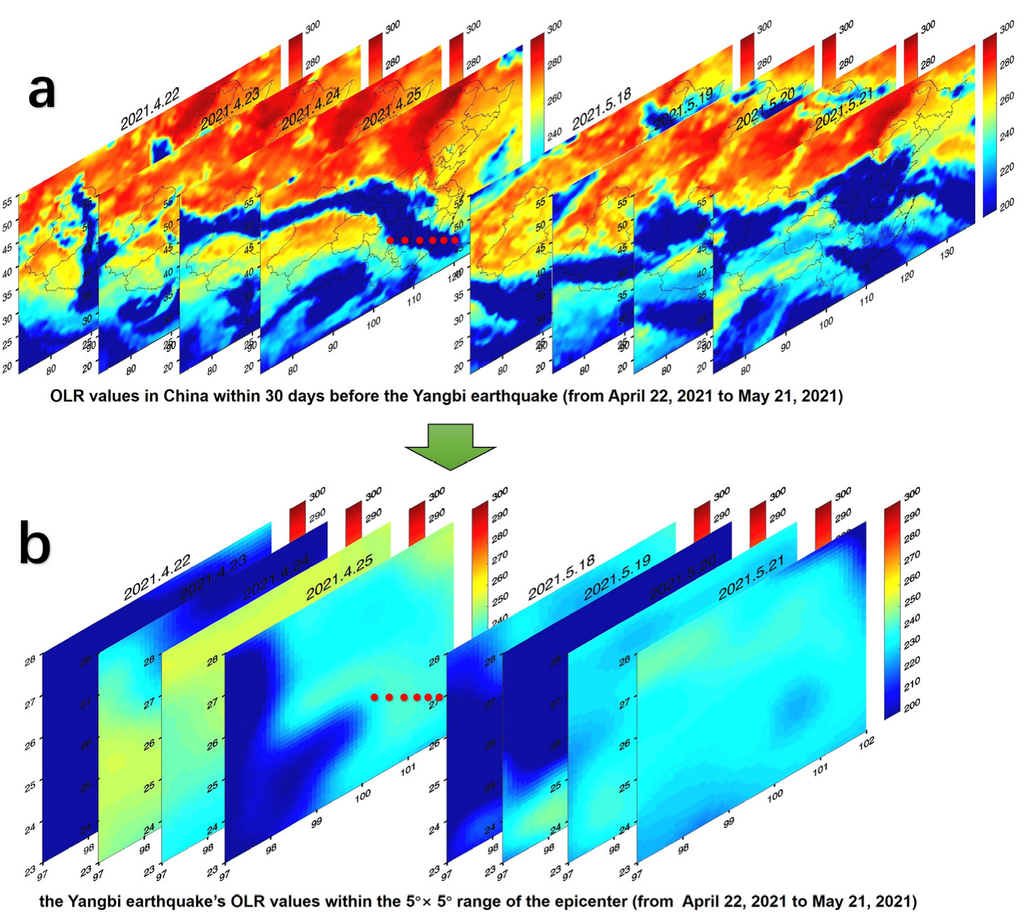
The original OLR data were organized in an array of 180 × 360 pixels. The time dimension was continuous. The a-plot in Figure 2 shows the OLR values for the region of China from 22 April 2022 to 21 May 2022. The b-plot in Figure 2 shows the Yangbi earthquake in the 5° × 5° area (5 × 5 pixels). Figure 2 was drawn in MATLAB. Extracting the experimental area from the original data was the main pre-processing method in this experiment.

3. Methods

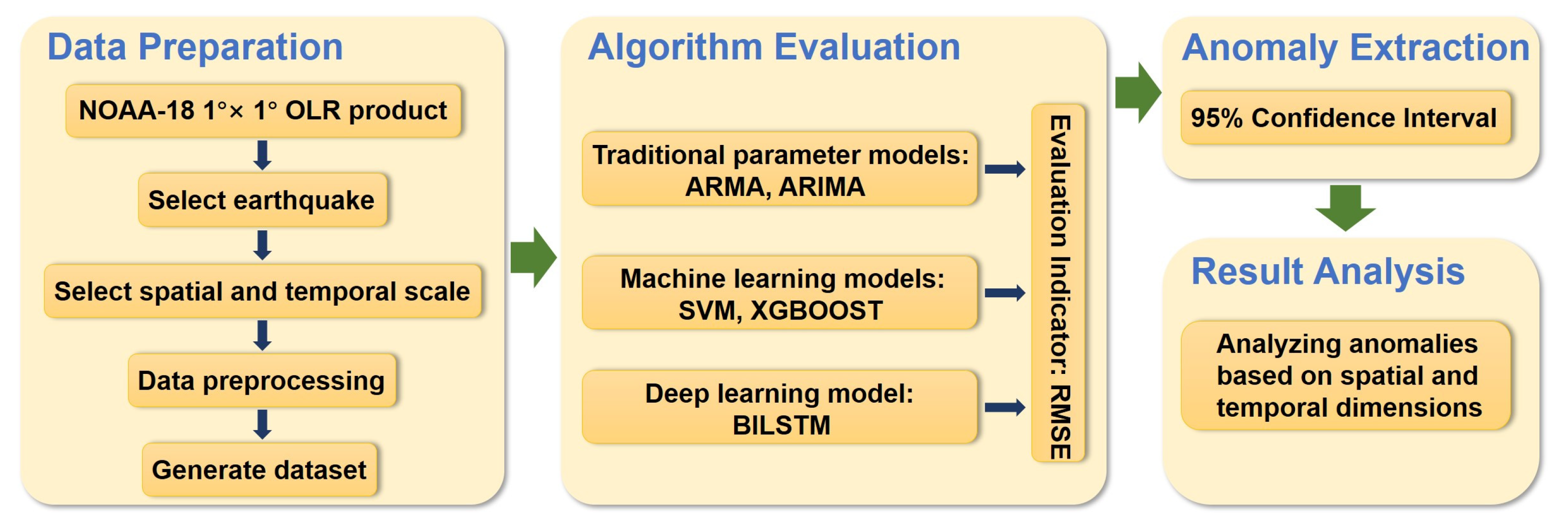
The existence of pre-earthquake thermal infrared anomalies has been demonstrated in many studies. Most traditional studies were based on different algorithms to extract the intensity and distribution range of thermal infrared anomalies in pre-earthquake time and spatial dimensions, such as the RST algorithm, wavelet vorticity method, and eddy field method [2,3,4]. The experiment was based on time series data of outgoing longwave infrared radiation and used a time series prediction model to predict the values of longwave infrared radiation at different time ranges before the earthquake within a specific spatial coverage of the epicenter. Data preparation involved downloading the data and selecting seismic examples and spatial and temporal scales. The data were cropped to the corresponding temporal and spatial scales to generate the dataset. By comparing and analyzing the prediction performance of different time series prediction models for different prediction periods, we selected the best performing model for the earthquake example study in the algorithm evaluation phase. In the anomaly extraction phase, the confidence interval was used as the evaluation criterion to extract the magnitude of the range outside the confidence interval and the corresponding date. Finally, the anomalies were analyzed based on the spatiotemporal dimension. Figure 3 shows the entire process of this experiment.

3.1. Time Series Forecasting Models

3.1.1. ARMA/ARIMA

ARMA and ARIMA models were obtained from a combination of autoregressive and moving average models [34]. When the time series is smooth, given a time series t = 0 , t = 1 , t = 2 , ARMA(p, q) can be expressed as
z t = m 1 z t 1 + + m p z t p + c t + n 1 c t 1 + + n q c t q
where m p 0 , n q 0 , z t is a stationary sequence, c t is a white noise sequence, p is the autoregressive parameter, and q is the moving average parameter. If the mean of z t is non-zero, then δ = μ 1 η 1 η p is set and (1) is rewritten as [35,36]:
z t = δ + m 1 z t 1 + + m p z t p + c t + n 1 c t 1 + + n q c t q
When the time series is not smooth, the difference term can be introduced to smooth the series, where ARMA(p, q) becomes ARMA(p, d, q). The “d” in ARMA(p, d, q) is called the difference order, and is usually differenced once or twice for an unsteady time series. The difference separates out the noise in the time series and replaces the time series value with the difference between the original and previous values [37].

3.1.2. SVM

Since Vapnik [38] developed support vector machines in 1995, the machine learning model has been widely used in pattern recognition, object classification, and time series regression tasks. Support vector regression models differ from traditional parametric models in that the former uses training data to obtain regression results [39]. Suppose that we have training data x 1 , y 1 , x 2 , y 2 , x l , y l , where x i is the input value and y i is the output value corresponding to it. Optimization problems in support vector regression are as follows:
m i n ω , b , ξ , ξ *         1 2 ω T ω + C i = 1 l ξ i + ξ i *
subject   to   y i ω T φ x i + b ϵ + ξ i * , ω T φ x i + b y i ϵ + ξ i                             ξ i , ξ i * 0 ,       i = 1 , , l
where ω is the normal vector, b is the intercept distance, x i is mapped by the function to a high-dimensional space, and ξ i * and ξ i are the upper and lower errors of the training respectively. The parameters controlling the regression quality are the cost error C , the width of the dimension ϵ , and the mapping function φ . SVR avoids under- and overfitting training data by minimizing the error and the canonical term. The dual problem of the function is treated next.
m i n α , α *       1 2 α α * T Q α α * + ϵ i = 1 l α i + α i * + i = 1 i y i α α i *
subject   to   i = 1 l α i α i * = 0         Q i j = φ x i T φ x j           0 α i ,             α i * C ,             i = 1 , , l
Faced with the problem of computing functions, we can introduce polynomial kernels or RBF kernels for efficient computation [40].

3.1.3. XGBoost

XGBoost is a machine learning model proposed by Tianqi Chen et al. [41]. It is an improvement on the gradient-boosting decision tree, which gives full play to the calculator’s parallel computing power and improves the algorithm’s accuracy. Suppose we have training data c 1 , d 1 , c 2 , d 2 , c s , d s , x r X R o , y r Y R , where X is the input space and Y is the output space corresponding to it. The optimization objective function L u of the XGBoost algorithm is:
L u = r = 1 s l d r , d ˜ r u 1 + f u c r ) + H f u
where d ˜ r u 1 is expressed as the predicted value of the model at the u 1 th iteration of the sample; f u c s is described as the predicted value of the model at the t th iteration of the sample; and H f u is the canonical term of the objective function. A Taylor expansion of the above equation gives:
L ˜ u j = 1 v e j r K j g r + 1 2 e j 2 r K j h r + λ + γ T
where g r and h r are the first- and second-order gradients of sample c r , respectively; e j is the output value of the j th node; λ and γ are the regular term coefficients; and K j is the subset of samples in the j th leaf node. The training process of the XGBoost model is the process of solving the above equation and finding the optimal solution [42].

3.1.4. BILSTM

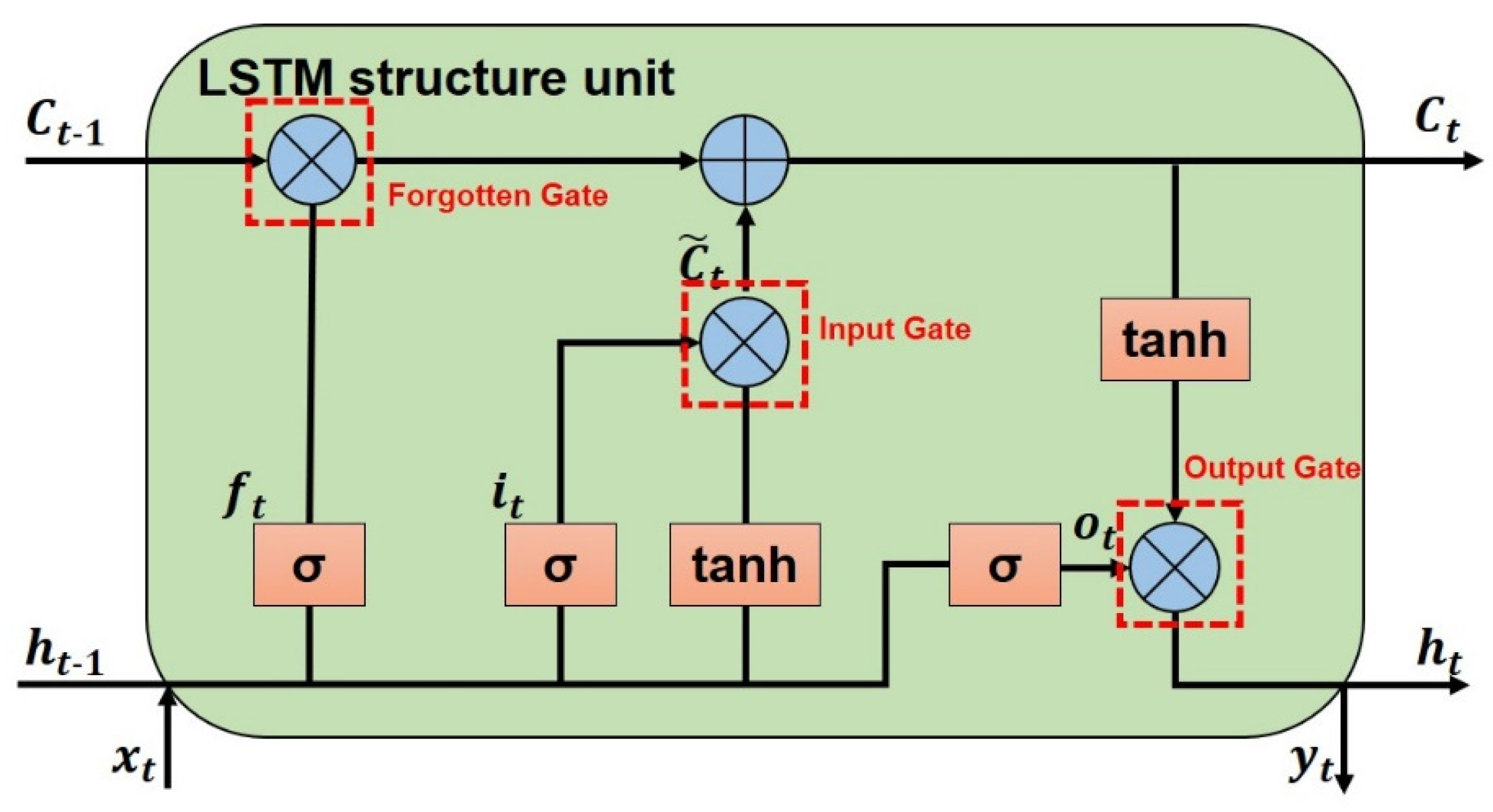
Recurrent neural networks (RNNs) are a sequence-to-sequence model where the model does not change depending on the length of the sequence. However, when dealing with long sequences, it forgets information from further back in time, leading to problems such as gradient loss and overfitting. The long short-term memory (LSTM) model improves on the RNN by adding “forgetting gates”, “input gates”, and “output gates” to control the retention and rejection of information through the function of gates. This optimizes the shortcomings of RNN’s short-term memory and can effectively handle the transfer of information in long-time sequences [43,44]. Figure 4 shows a structural diagram of the LSTM model.
The BILSTM model, a bidirectional long short-term memory neural network, consists of two independent LSTM models, a forward model and a backward model. The output combines the results of both models. To some extent, the BILSTM model can compensate for information that may be missed by the unidirectional LSTM [45]. Figure 5 shows a structural diagram of the BILSTM model.

3.2. Anomaly Assessment Method

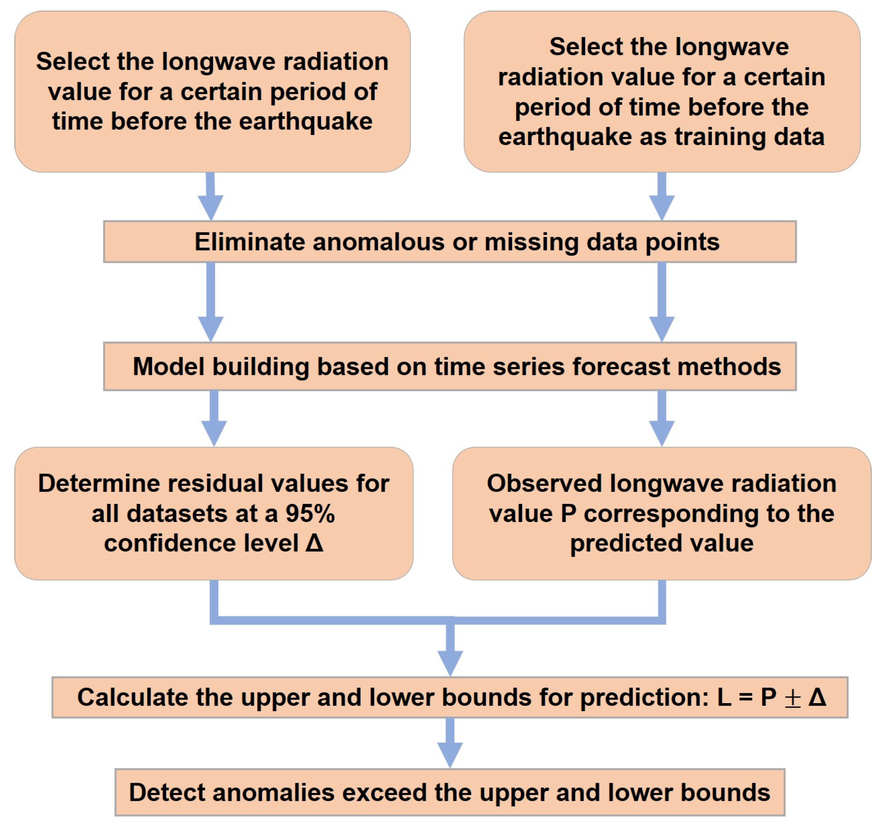
The confidence level, which belongs to statistics, has also been widely used in the earthquake field. Yu et al. [46] studied the load/unload response ratio (LURR) time series before earthquakes and found that the confidence level of LURR anomalies was highly correlated with the occurrence of large earthquakes. LURR precursor anomalies preceded most earthquakes with a probability higher than 90%. Alam et al. [47] used a confidence interval of 95% for anomaly selection in a statistical analysis of radon data from the Wenchuan earthquake in their analysis of the global seismic activity in 12 scenarios by magnitude and period. Yin et al. [48] found a significant activity cycle of about 50 years with a confidence level well above 95%. Kutoglu et al. [49] used the 95% confidence level as an anomaly test in their analysis of aerosol optical depth (AOD) time series data. Zhang et al. [50] proposed a new method for pre-seismic TEC detection using the time series method, in which the difference between the predicted and actual values of the time series prediction model was presented. The upper and lower limits were the residual values with a statistical ratio above 95%. The range was obtained by adding and subtracting from the predicted value, and any actual value outside this range was considered an anomaly. Zhai et al. [23] also applied this method to detect anomalies in a pre-earthquake longwave radiation time series and successfully detected significant anomalies. We have made improvements to the above methods. We trained several days of data and predicted OLR values for the corresponding number of days. Then, we calculated the residual value of the original data and obtained the 95% confidence interval of the predicted value. When the true value exceeded the upper or lower bound of the confidence interval, the datapoint was determined as an anomaly. Figure 6 shows the detailed anomaly extraction method process.
Using the Luding earthquake 31.5° N 102.5° E grid data as an example, 95% confidence intervals were calculated for the predicted values after the use of the time series to predict the longwave radiation values. The red curve shows the predicted value 30 days before the earthquake, and the blue curve shows the upper 95% confidence interval, the light blue curve shows the lower 95% confidence interval, and the green curve shows the true value of the grid. In the graphs, we considered the longwave radiation values to be anomalous if the actual values were below the lower bound of the interval or above the upper bound of the interval. For the 31.5° N 102.5° E grid of the Luding earthquake, Figure 7 shows the predicted OLR values and the anomaly performance.

4. Results

4.1. Analysis of Algorithm Evaluation Results

We have chosen the Yangbi earthquake as a study earthquake example. Different training and test data were selected to predict and calculate the error on the grid data within 5° × 5° for this earthquake example. For the evaluation of the performance of the different algorithms, the data need to be divided into training data and test data. Based on previous conclusions, the time of occurrence of pre-seismic thermal anomalies is irregular. In general, they occur within six months prior to the earthquake. We aimed to study close-proximity anomalies, so we chose the 30 days before the earthquake as the prediction days. Due to the lag in data acquisition and our desire to obtain the long time series distribution of the anomalies for future practical applications, our test data were sourced from 5, 10, 15, 20, 25, and 30 days before the earthquake. The OLR data are seasonal. A training period of one year was found to work best when Zhai et al. [23] investigated the predictive performance of OLR based on different algorithms. Data from the year before the earthquake can reduce the disturbance of seismic anomalies to some extent. Therefore, we chose the training data in this experiment to be one year (360 days) ahead of the test data. Taking the Yangbi earthquake on 21 May 2021, for example, 5-day training data: 22 May 2020–16 May 2021, test data: 17–21 May 2021, 10-day training data: 17–11 May 2021, test data: 12–21 May 2021, and so on. The study area of the algorithm is shown in Figure 1. As the original data provided data located at a 1° × 1° centroid, the location was recorded in the form of 25.5° N 99.5° E. The root mean square error is a common error test and has been widely used in earthquake prediction research [13,14,15,19,51]. The experiment uses the root mean square error (RMSE) to assess the error between the predicted and actual values. The total error is calculated for the same number of days tested.
Table 2 shows the error results of the BILSTM algorithm for different days and grid points. The remaining ARMA, ARIMA, SVM, and XGBoost algorithms were evaluated separately, and the total error of the different algorithms was analyzed following the same steps as described above; not all values are shown in the paper for the sake of brevity. Table 3 shows the total RMSE for all grids of the five algorithms for different forecast days.
Table 3 shows that the total sum of root mean square errors for all algorithms was the smallest for the 5-day prediction time; the BILSTM algorithm had the smallest sum of root mean square errors for the 5-day prediction time. Therefore, BILSTM was selected as the research algorithm for this experiment. Five days was chosen as the prediction time. Five days was a short prediction time, and we used the sliding time window method [51] in this specific experiment to achieve a prediction of thirty days.

4.2. Analysis of Anomaly Results of Earthquake Cases

The best performing BILSTM prediction model was selected as the prediction algorithm after the error analysis of different algorithms and different prediction days. We then used the anomaly assessment method to study the Yangbi Ms6.4-magnitude earthquake on 21 May 2021 and the Luding Ms6.8-magnitude earthquake on 5 September 2022. The following graphs show the predicted results for two examples of earthquakes.
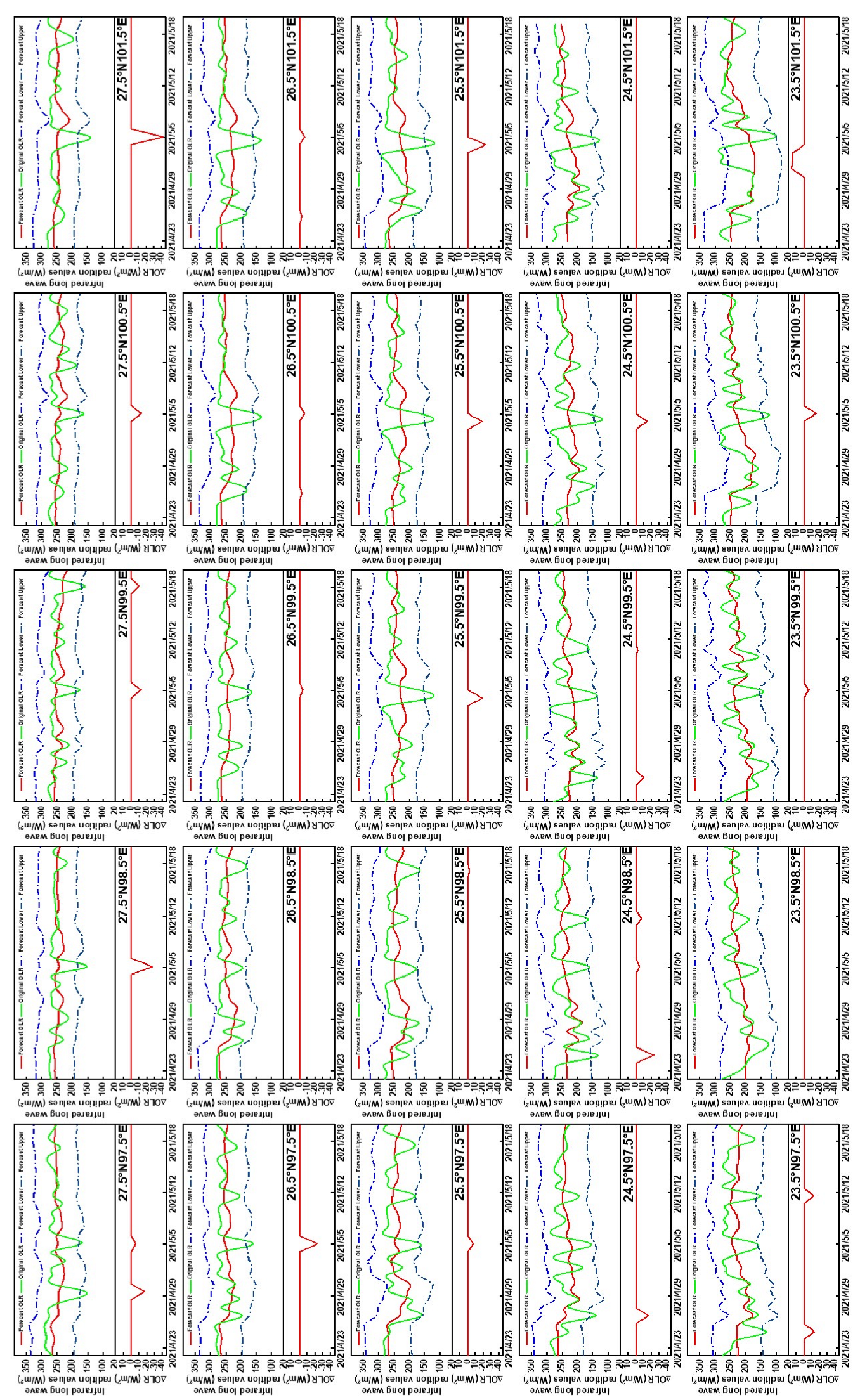
The green curve shows the actual value; the red curve shows the predicted value; the blue curve shows the upper bound of the confidence interval; the light blue curve shows the lower bound of the confidence interval; and the red dashed line in the subplots indicates the difference between exceeding the upper bound and falling below the lower bound. Figure 8 shows that within the 5° × 5° area, 22 grid points, excluding grids points 23.5° N 98.5° E, 24.5° N 101.5° E, and 26.5° N 98.5° E, provided one to three cases of varying amounts outside the confidence interval in the month before the earthquake. Of these, 24 grid points were below the lower bound of the confidence interval, with the exception of the 23.5° N 101.5° E point, which was above the upper bound. The maximum value below the lower confidence interval was found at grid point 27.5° N 101.5° E, northeast of the epicenter. Therefore, we speculated that in the month before the Yangbi earthquake, anomalies of varying sizes were prevalent in the 5° × 5° area near the epicenter, dominated by those below the lower confidence interval.
Figure 8 shows that most of the anomalies are below the lower bound of the confidence interval. To better illustrate how much the range was exceeded, the vertical coordinates in Figure 9 are negative upwards and positive downwards. Figure 9 shows that smaller-scale and smaller-range anomalies were observed during the two time periods from 25 April to 26 April and from 11 May to 12 May. A large-scale and more robust anomaly was observed from 5 May to 6 May, with the anomaly covering 17 grids, and the radiative energy of individual grid points was exceeded by up to 42.27 W / m 2 , 27.52 W / m 2 , 23.58 W / m 2 , and 23.11 W / m 2 . Therefore, we speculated that a strong and concentrated OLR anomaly existed 15 to 16 days before the Yangbi earthquake (5–6 May).
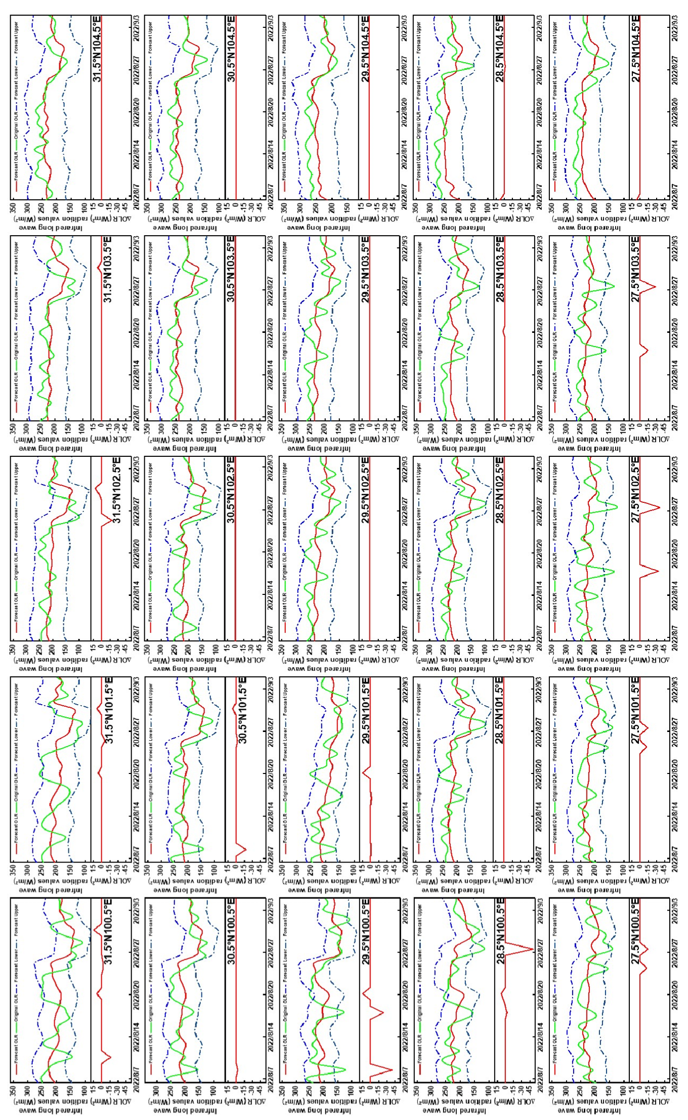
Figure 10 shows that nine grid points did not exceed the confidence interval and were mainly located near the epicenter and to the east. Combined with Figure 1, it can be seen that the eastern part of the epicenter is the Chengdu Plain, which is at a lower elevation and has relatively inactive fault zone activity with fewer anomalies. The coexistence of anomalies above and below confidence intervals occurred at several grid points. The maximum value below the lower boundary occurs at the 28.5° N 100.5° E grid point southwest of the epicenter. Therefore, we speculated that the anomalies near the epicenter one month before the Luding earthquake were mainly distributed southwest and northwest of the epicenter. Both anomaly types below the lower confidence interval and above the upper confidence interval occurred.
As shown in Figure 11, anomalies of different intensity, type, and extent were present on 9 August, 11 August, 18 August, 20 August to 21 August, 25 August to 26 August, 28 August, and 31 August. The maximum radiation exceedance on 9 August, 18 August, and August 28 reached 40.08 W / m 2 , 34.08 W / m 2 , and 51.52 W / m 2 , respectively. We, therefore, speculated that there were several OLR anomalies of high intensity in the month before the Luding earthquake.

5. Discussion

Many studies have shown the presence of infrared longwave anomalies before earthquakes, but these studies have limitations. Researchers have obtained good anomaly predictions in different case studies using different methods and data, but similar results may not be obtained with a different method, data, or case. Xie et al. [52] used the two-year relative wavelet power spectrum method, and Wei et al. [53] used the wavelet power spectrum method based on FY-2E bright temperature data to study the 14 April 2010 Yushu Ms7.1 earthquake in China. The spatial distribution and intensity of the anomaly spatiotemporal evolution results obtained by the two differed significantly. Sun et al. [9] found no significant anomalies when they studied the 25 April 2015 Ms8.1 earthquake in Nepal using the RST algorithm and OLR data. However, Zhang et al. [54] obtained good anomaly prediction performance near the epicenter when studying the same earthquake case using the power spectrum method and bright temperature data. In addition, traditional methods for studying anomalies in longwave radiation data have been biased towards the representation of thermal anomalies, such as the RST algorithm, where values less than zero are ignored in the calculation of the Alice index [55].
Addressing the two limitations mentioned above, the method of this paper is innovative in two ways. The traditional thermal anomaly extraction model is only a model. In contrast, the BILSTM time series prediction model used is a deep learning model with the ability to train data and learn data, which is a data-driven approach. The training process does not change the original data for earthquake cases and data sources. The model can learn the data trend in the period before the earthquake. In the prediction process, the model parameters are modified to make the predicted value as close to the actual value as possible to achieve a better prediction result. The anomaly detection method used calculates 95% confidence intervals for the OLR, forming several ranges with upper and lower bounds. True values falling within this range are considered to be free of anomalies, while true values above the upper bound or below the lower bound are considered to be anomalous. This approach implies that there are two different types of anomalies. If the anomaly is above the upper bound, we consider it to be a hot anomaly, and if the anomaly is below the lower bound, we consider it to be a cold anomaly. While traditional methods can only show anomalies of high longwave radiation values, our method has both hot and cold anomalies, subdividing the types of anomalies that exist before the earthquake [2,3]. We have tried to explain cold anomalies at a physical level. According to the results of the rock experiments, compression leads to an increase in temperature, and tension leads to a decrease in temperature. The location of the Yangbi earthquake and the results of a multi-period GNSS strain rate field based on GPS data indicate that the Yangbi earthquake is located in a tension zone; the Luding earthquake is in a zone of weakness at the high-value edge of the shear strain of a large strike-slip fault zone and a zone of tensor strain perpendicular to the fault direction.
Lithosphere–Atmosphere–Ionosphere Coupling (LAIC) was used to explain the physical and chemical mechanisms of the various anomalies that appear at the surface, in the atmosphere, and in the ionosphere during the gestation and occurrence of earthquakes [56]. It was found that there was a relationship between pre-earthquake OLR and ionospheric anomalies, which can be explained by LAIC [57,58,59]. Fu et al. studied strong earthquakes with magnitudes greater than 6 in Taiwan and concluded that seismic OLR anomalies may originate from electromagnetic radiation as well as gas emissions [60]. We tried to compare anomalous the OLR results of the two earthquakes with the anomalous results of TEC obtained by other scholars. Zhai et al. [23] used the ARMA model to predict the longwave radiation values of the 8 August 2017 Jiuzhaigou Ms7.0 earthquake and found OLR anomalies at the epicenter on 27 July and 5 August; Zhu et al. [61] used the sliding quartile to detect ionospheric TEC anomalies for the same earthquake and found TEC anomalies on 28 July, 4 August, and 6 August; the timing of OLR anomalies and of ionospheric anomalies were close. Du et al. [62] used Chinese seismo-electromagnetic satellite data to detect electron density anomalies of the Yangbi Ms6.4 earthquake in Yunnan on 21 May 2021 and found anomalies on 5 May and 8 May; Dong et al. [63] used ionospheric TEC data to study the same earthquake case and detected the strongest anomaly near the epicenter on 5 May. We found strong and concentrated OLR anomalies from 5 May to 6 May before the Yangbi earthquake. The timing of the OLR anomalies is also very close to that of the ionospheric anomalies detected before the Yangbi Ms6.4 earthquake. Therefore, we believe that there is a specific link exists between the OLR anomaly and the ionospheric anomaly that existed before the earthquake.
In this paper, we only selected the Yangbi Ms6.4 earthquake of 21 May 2021 and the Luding Ms6.8 earthquake of 5 September 2022 for study. The number of earthquake cases was too low to form a statistical analysis of the method. We detected significant anomalies within a 5° × 5° area of the epicenter and a month before the earthquake with the parameters of the earthquake case study determined with reference to the summary of previous works. It was not possible to determine whether such anomalies existed beyond this range and time period. The distribution and timing of pre-earthquake anomalies varied between different-magnitude earthquakes, and specific study areas and times need to be delineated based on specific earthquake examples. The rapid development of deep learning has led to more and better time series prediction models, such as the Transformer algorithm [64,65], a complex time series algorithm that can better predict OLR values and reduce errors. In addition, the parameter setting of the model was also an important factor affecting good and bad errors, and different parameters give different results. The experiment needed to establish the optimal set of model parameters. In future research, we need to improve and refine the above-mentioned drawbacks.

6. Conclusions

This paper used OLR data to predict 30-day values before the Yangbi Ms6.4-magnitude earthquake on 21 May 2021 and the Luding Ms6.8-magnitude earthquake on 5 September 2022 based on a time series prediction model and the sliding time window method and assessed the anomalies using 95% confidence intervals. Five time series prediction models were used to calculate the RMSE for 5, 10, 15, 20, 25, and 30 days in 25 grids using the Yangbi earthquake as an evaluation example. The total RMSE of the BILSTM model for the 5-day prediction time was 619.2920, which was smaller than any other combination of model and number of days. The following conclusions can be drawn:
(1) The anomaly distributions of the Yangbi and Luding earthquakes were large. There was a correspondence between the anomaly distribution area and the distribution of fault zones. The magnitude of the anomalies of the two earthquakes was significant, and both earthquakes had showed anomaly values above 40. The anomalies of the two earthquakes showed different characteristics in the time dimension. The Yangbi earthquake anomaly appeared 15 to 16 days before the earthquake (5–6 May) with a higher intensity and more concentrated temporal distribution. The Luding earthquake showed stronger anomalies 27 (9 August), 18 (18 August), and 8 (28 August) days before the earthquake. The temporal distribution was more scattered. Overall, OLR data based on time series could effectively detect apparent pre-earthquake anomalies and analyze the possibility of earthquake generation by the characteristics presented by the anomalies, which was a promising method for earthquake prediction.
(2) Based on the time series prediction model to study the seismic anomalies in the 5° × 5° area and within one pre-earthquake time period, we found that the Yangbi and Luding earthquakes have specific anomaly characteristics and show similar but not identical anomaly distributions. However, we may find anomalies with the same characteristics in different cases by studying many earthquake cases. This experimental anomaly extraction method used a 95% confidence interval, and there were many small and heterogeneous distribution characteristics in the results of the studied earthquake anomalies. These anomalies were minor in degree and in terms of indicative features, which may affect the interpretation of the overall seismic anomaly and need to be eliminated. Overall, the study of multiple cases based on time series prediction models is a direction for future anomaly research. The best confidence interval setting must be found in numerous cases and studies to summarize the potential patterns between the characteristics of the OLR anomaly distribution and earthquake occurrence.

Author Contributions

Conceptualization, J.Z. (Junqing Zhu) and K.S.; methodology, J.Z. (Junqing Zhu); software, J.Z. (Junqing Zhu); validation, J.Z. (Junqing Zhu), J.Z. (Jingye Zhang), and K.S.; formal analysis, J.Z. (Jingye Zhang); investigation, J.Z. (Jingye Zhang); resources, J.Z. (Junqing Zhu); writing—original draft preparation, J.Z. (Junqing Zhu); writing—review and editing, J.Z. (Junqing Zhu); visualization, J.Z. (Jingye Zhang); supervision, K.S.; project administration, K.S.; funding acquisition, K.S. All authors have read and agreed to the published version of the manuscript.

Funding

This work was funded by the National Natural Science Foundation of China under Grant No. U2039202, and the National Key Research and Development Program of China under Grant No. 2019YFC1509202.

Institutional Review Board Statement

Not applicable.

Informed Consent Statement

Not applicable.

Data Availability Statement

This study uses NOAA-18 satellite 1° × 1° OLR data that can be downloaded via NCEP’s FTP server (ftp://ftp.cpc.ncep.noaa.gov/precip/noaa18_1x1/) (accessed on 20 December 2022).

Acknowledgments

We thank the National Natural Science Foundation of China and the National Key Research and Development Program of China for funding this study. We thank NOAA for providing the OLR data and Sha Yin for guidance in producing the figures.

Conflicts of Interest

The authors declare no conflict of interest.

References

  1. Gornyy, V.; Sal’man, A.; Tronin, A.; Shilin, B. Outgoing terrestrial infrared radiation as an indicator of seismic activity. Dokl. Akad. Nauk USSR 1988, 301, 67–69. (In Russian) [Google Scholar]
  2. Lu, X.; Meng, Q.; Gu, X.; Zhang, X.; Xie, T.; Geng, F. Thermal infrared anomalies associated with multi-year earthquakes in the Tibet region based on China’s FY-2E satellite data. Adv. Space Res. 2016, 58, 989–1001. [Google Scholar] [CrossRef]
  3. Zhang, Y.; Meng, Q. A statistical analysis of TIR anomalies extracted by RSTs in relation to an earthquake in the Sichuan area using MODIS LST data. Nat. Hazards Earth Syst. Sci. 2019, 19, 535–549. [Google Scholar] [CrossRef] [Green Version]
  4. Xiong, P.; Shen, X.H.; Bi, Y.X.; Kang, C.L.; Chen, L.Z.; Jing, F.; Chen, Y. Study of outgoing longwave radiation anomalies associated with Haiti earthquake. Nat. Hazards Earth Syst. Sci. 2010, 10, 2169–2178. [Google Scholar] [CrossRef] [Green Version]
  5. Kong, X.; Bi, Y.; Glass, D.H. Detecting seismic anomalies in outgoing long-wave radiation data. IEEE J. Sel. Top. Appl. Earth Obs. Remote Sens. 2014, 8, 649–660. [Google Scholar] [CrossRef]
  6. Mahmood, I.; Iqbal, M.F.; Shahzad, M.I.; Qaiser, S. Investigation of atmospheric anomalies associated with Kashmir and Awaran Earthquakes. J. Atmos. Sol.-Terr. Phys. 2017, 154, 75–85. [Google Scholar] [CrossRef]
  7. Natarajan, V.; Philipoff, P.; Sreedharan, V.W.; Venkatachalapathy, H. Observation of pre-earthquake thermal signatures using geostationary satellites: Implications for earthquake forecasting. J. Appl. Remote Sens. 2016, 10, 46004. [Google Scholar] [CrossRef]
  8. Prakash, R.; Srivastava, H. Diurnal variations of outgoing long wave radiation (OLR) vis a vis 4 January, 2016 Manipur earthquake (Mw: 6.7): An earthquake precursor? Mausam 2017, 68, 475–486. [Google Scholar] [CrossRef]
  9. Sun, K.; Shan, X.-J.; Ouzounov, D.; Shen, X.-H.; Jing, F. Analyzing long wave radiation data associated with the 2015 Nepal earthquakes based on Multi-orbit satellite observations. Chin. J. Geophys. 2017, 60, 3457–3465. [Google Scholar]
  10. Ouzounov, D.; Liu, D.; Chunli, K.; Cervone, G.; Kafatos, M.; Taylor, P. Outgoing long wave radiation variability from IR satellite data prior to major earthquakes. Tectonophysics 2007, 431, 211–220. [Google Scholar] [CrossRef]
  11. Ohring, G.; Gruber, A. Satellite radiation observations and climate theory. In Advances in Geophysics; Elsevier: Amsterdam, The Netherlands, 1983; Volume 25, pp. 237–304. [Google Scholar]
  12. Yang, H.M.; Pan, Z.S.; Wei, B.; Of, S. Review of Time Series Prediction Methods. Comput. Sci. 2019, 46, 21–28. [Google Scholar]
  13. Saqib, M.; Senturk, E.; Sahu, S.A.; Adil, M.A. Ionospheric anomalies detection using autoregressive integrated moving average (ARIMA) model as an earthquake precursor. Acta Geophys. 2021, 69, 1493–1507. [Google Scholar] [CrossRef]
  14. Saqib, M.; Senturk, E.; Sahu, S.A.; Adil, M.A. Comparisons of autoregressive integrated moving average (ARIMA) and long short term memory (LSTM) network models for ionospheric anomalies detection: A study on Haiti (M-w=7.0) earthquake. Acta Geod. Geophys. 2022, 57, 195–213. [Google Scholar] [CrossRef]
  15. Senturk, E.; Saqib, M.; Adil, M.A. A Multi-Network based Hybrid LSTM model for ionospheric anomaly detection: A case study of the M-w 7.8 Nepal earthquake. Adv. Space Res. 2022, 70, 440–455. [Google Scholar] [CrossRef]
  16. Yue, Y.; Koivula, H.; Bilker-Koivula, M.; Chen, Y.; Chen, F.; Chen, G. TEC Anomalies Detection for Qinghai and Yunnan Earthquakes on 21 May 2021. Remote Sens. 2022, 14, 4152. [Google Scholar] [CrossRef]
  17. Xiong, P.; Zhai, D.; Long, C.; Zhou, H.; Zhang, X.; Shen, X. Long short-term memory neural network for ionospheric total electron content forecasting over China. Space Weather. 2021, 19, e2020SW002706. [Google Scholar] [CrossRef]
  18. Mohammed, D.H.K.; Kulahci, F.; Muhammed, A. Determination of possible responses of Radon-222, magnetic effects, and total electron content to earthquakes on the North Anatolian Fault Zone, Turkiye: An ARIMA and Monte Carlo Simulation. Nat. Hazards 2021, 108, 2493–2512. [Google Scholar] [CrossRef]
  19. Mir, A.A.; Celebi, F.V.; Alsolai, H.; Qureshi, S.A.; Rafique, M.; Alzahrani, J.S.; Mahgoub, H.; Hamza, M.A. Anomalies Prediction in Radon Time Series for Earthquake Likelihood Using Machine Learning-Based Ensemble Model. IEEE Access 2022, 10, 37984–37999. [Google Scholar] [CrossRef]
  20. Feng, X.; Zhong, J.; Yan, R.; Zhou, Z.; Tian, L.; Zhao, J.; Yuan, Z. Groundwater radon precursor anomalies identification by EMD-LSTM model. Water 2022, 14, 69. [Google Scholar] [CrossRef]
  21. Roebeling, R.; Schulz, J.; Hewison, T.; Theodore, B. Inter-calibration of METEOSAT IR and WV channels using HIRS. AIP Conf. Proc. 2013, 1531, 288–291. [Google Scholar]
  22. Turner, E.C.; Tett, S.F. Using longwave HIRS radiances to test climate models. Clim. Dyn. 2014, 43, 1103–1127. [Google Scholar] [CrossRef]
  23. Zhai, D.; Zhang, X.; Xiong, P. Detecting thermal anomalies of earthquake process within outgoing longwave radiation using time series forecasting models. Ann. Geophys. 2020, 63, PA548. [Google Scholar] [CrossRef]
  24. Ellingson, R.G.; Yanuk, D.J.; Lee, H.-T.; Gruber, A. A technique for estimating outgoing longwave radiation from HIRS radiance observations. J. Atmos. Ocean. Technol. 1989, 6, 706–711. [Google Scholar] [CrossRef]
  25. Lee, H.-T.; Ellingson, R.G. HIRS OLR climate data record–production and validation updates. AIP Conf. Proc. 2013, 1531, 420–423. [Google Scholar]
  26. Chen, Q.F.; Zheng, D.L.; Che, S. Earthquake Cases in China (1992–1994); Seismological Press: Beijng, China, 2002. [Google Scholar]
  27. Chen, Q.F.; Zheng, D.L.; Liu, G.P.; Li, M. Earthquake Cases in China (1995–1996); Seismological Press: Beijing, China, 2002. [Google Scholar]
  28. Jiang, H.K.; Fu, H.; Yang, M.L.; Ma, H.S. Earthquake Cases in China (2003–2006); Seismological Press: Beijing, China, 2014. [Google Scholar]
  29. Jing, F.; Shen, X.; Kang, C.; Meng, Q.; Xiong, P. Anomalies of outgoing longwave radiation before some medium to large earthquakes. Earthquake 2009, 29, 117–122. [Google Scholar]
  30. Feng, J.; Xuhui, S.; Hui, W.; Chunli, K.; Pan, X. Infrared characteristics analysis of the 2015 Nepal M S 8.1 earthquake. Acta Seismol. Sin. 2016, 38, 429–437. [Google Scholar]
  31. Song, D.; Zang, L.; Shan, X.; Yuan, Y.; Cui, J.; Shao, H.; Shen, C.; Shi, H. A study on the algorithm for extracting earthquake thermal infrared anomalies based on the yearly trend of LST. Seismol. Geol. 2016, 38, 680–695. [Google Scholar]
  32. He, S.; Zhou, Q.; Liu, Z. Seismogenic Structure of the 2021 Yangbi, Yunnan MS6.4 Earthquake and Earthquake Risk Analysis in the Epicenter Area. J. Seismol. Res. 2021, 44, 380–390. [Google Scholar]
  33. Fan, X.; Wang, X.; Dai, L.; Fang, C.; Deng, Y.; Zou, C.; Tang, M.; Wei, Z.; Dou, X.; Zhang, J. Characteristics and spatial distribution pattern of M S 6.8 Luding earthquake occurred on September 5, 2022. J. Eng. Geol. 2022, 30, 1504–1516. [Google Scholar]
  34. Valipour, M.; Banihabib, M.E.; Behbahani, S.M.R. Comparison of the ARMA, ARIMA, and the autoregressive artificial neural network models in forecasting the monthly inflow of Dez dam reservoir. J. Hydrol. 2013, 476, 433–441. [Google Scholar] [CrossRef]
  35. Kumar, U.; Jain, V. ARIMA forecasting of ambient air pollutants (O 3, NO, NO 2 and CO). Stoch. Environ. Res. Risk Assess. 2010, 24, 751–760. [Google Scholar] [CrossRef]
  36. Shumway, R.H.; Stoffer, D.S.; Stoffer, D.S. Time Series Analysis and Its Applications; Springer: Berlin/Heidelberg, Germany, 2000; Volume 3. [Google Scholar]
  37. Zhang, H.; Zhang, S.; Wang, P.; Qin, Y.; Wang, H. Forecasting of particulate matter time series using wavelet analysis and wavelet-ARMA/ARIMA model in Taiyuan, China. J. Air Waste Manag. Assoc. 2017, 67, 776–788. [Google Scholar] [CrossRef] [PubMed] [Green Version]
  38. Vapnik, V. The Nature of Statistical Learning Theory; Springer Science & Business Media: Berlin/Heidelberg, Germany, 1999. [Google Scholar]
  39. Sapankevych, N.I.; Sankar, R. Time series prediction using support vector machines: A survey. IEEE Comput. Intell. Mag. 2009, 4, 24–38. [Google Scholar] [CrossRef]
  40. Chen, B.-J.; Chang, M.-W. Load forecasting using support vector machines: A study on EUNITE competition 2001. IEEE Trans. Power Syst. 2004, 19, 1821–1830. [Google Scholar] [CrossRef] [Green Version]
  41. Chen, T.; Guestrin, C. Xgboost: A scalable tree boosting system. In Proceedings of the 22nd ACM Sigkdd International Conference on Knowledge Discovery and Data Mining, San Francisco, CA, USA, 13–17 August 2016; pp. 785–794. [Google Scholar]
  42. LI, H.; ZHU, Y. Xgboost algorithm optimization based on gradient distribution harmonized strategy. J. Comput. Appl. 2020, 40, 1633. [Google Scholar]
  43. Hochreiter, S.; Schmidhuber, J. Long short-term memory. Neural Comput. 1997, 9, 1735–1780. [Google Scholar] [CrossRef]
  44. Yan, X.; Shi, Z.; Wang, G.; Zhang, H.; Bi, E. Detection of possible hydrological precursor anomalies using long short-term memory: A case study of the 1996 Lijiang earthquake. J. Hydrol. 2021, 599, 126369. [Google Scholar] [CrossRef]
  45. Lin, H.; Zhang, S.; Li, Q.; Li, Y.; Li, J.; Yang, Y. A new method for heart rate prediction based on LSTM-BiLSTM-Att. Measurement 2023, 207, 112384. [Google Scholar] [CrossRef]
  46. Yu, H.Z.; Zhu, Q.Y. A probabilistic approach for earthquake potential evaluation based on the load/unload response ratio method. Concurr. Comput. Pract. Exp. 2010, 22, 1520–1533. [Google Scholar] [CrossRef]
  47. Alam, A.; Wang, N.; Zhao, G.; Barkat, A. Implication of radon monitoring for earthquake surveillance using statistical techniques: A case study of Wenchuan earthquake. Geofluids 2020, 2020, 2429165. [Google Scholar] [CrossRef]
  48. Yin, J.; Song, Z.; Xue, Y.; Liu, J.; Zhang, G.; Zhu, Y. Analysis on global huge earthquake activity. Acta Seismol. Sin. 2012, 34, 191–201. [Google Scholar]
  49. Kutoglu, S.H.; Ghasempour, F.; Sekertekin, A. Investigation of Possible MODIS AOD Anomalies as Earthquake Precursors for Global Earthquakes. Adv. Space Res. 2021, 68, 3531–3545. [Google Scholar] [CrossRef]
  50. Zhang, X.; Ren, X.; Wu, F.; Chen, Y. A New Method for Detection of Pre-Earthquake Ionospheric Anomalies. Chin. J. Geophys. 2013, 56, 213–222. [Google Scholar]
  51. Xiong, P.; Tong, L.; Zhang, K.; Shen, X.; Battiston, R.; Ouzounov, D.; Iuppa, R.; Crookes, D.; Long, C.; Zhou, H. Towards advancing the earthquake forecasting by machine learning of satellite data. Sci. Total Environ. 2021, 771, 145256. [Google Scholar] [CrossRef]
  52. Xie, T.; Kang, C.L.; Ma, W.Y. Thermal infrared brightness temperature anomalies associated with the Yushu (China) Ms = 7.1 earthquake on 14 April 2010. Nat. Hazards Earth Syst. Sci. 2013, 13, 1105–1111. [Google Scholar] [CrossRef] [Green Version]
  53. Wei, C.; Zhang, Y.; Guo, X.; Qin, M.; Ning, Y.-L.; Gao, J. Thermal infrared and long-wave radiation anomalies of Yushu MS 7.1 earthquake. Prog. Geophys. 2013, 28, 2444–2452. [Google Scholar]
  54. Zhang, X.; Zhang, Y.; Guo, X.; Wei, C.; Zhang, L. Analysis of thermal infrared anomaly in the Nepal MS8.1 earthquake. Earth Sci. Front. 2017, 24, 227–233. [Google Scholar]
  55. Tramutoli, V. Robust AVHRR Techniques (RAT) for environmental monitoring: Theory and applications. In Earth Surface Remote Sensing II; SPIE: Bellingham, WA, USA, 1998; pp. 101–113. [Google Scholar]
  56. Pulinets, S.; Ouzounov, D.; Karelin, A.; Davidenko, D. Lithosphere-atmosphere-ionosphere-magnetosphere coupling-a concept for pre-earthquake signals generation. In Pre-Earthquake Processes: A Multidisciplinary Approach to Earthquake Prediction Studies; American Geophysical Union: Washington, DC, USA, 2018; pp. 77–98. [Google Scholar]
  57. Parrot, M.; Tramutoli, V.; Liu, T.J.; Pulinets, S.; Ouzounov, D.; Genzano, N.; Lisi, M.; Hattori, K.; Namgaladze, A. Atmospheric and ionospheric coupling phenomena associated with large earthquakes. Eur. Phys. J. Spec. Top. 2021, 230, 197–225. [Google Scholar] [CrossRef]
  58. Conti, L.; Picozza, P.; Sotgiu, A. A critical review of ground based observations of earthquake precursors. Front. Earth Sci. 2021, 9, 676766. [Google Scholar] [CrossRef]
  59. Lu, J.; Hu, Y.; Jiang, C.; Zhao, Z.; Zhang, Y.; Ma, Z. Analysis of Pre-Earthquake Ionospheric Anomalies in the Japanese Region Based on DEMETER Satellite Data. Universe 2023, 9, 229. [Google Scholar] [CrossRef]
  60. Fu, C.-C.; Lee, L.-C.; Ouzounov, D.; Jan, J.-C. Earth’s outgoing longwave radiation variability prior to M≥ 6.0 earthquakes in the Taiwan area during 2009–2019. Front. Earth Sci. 2020, 8, 364. [Google Scholar] [CrossRef]
  61. Zhu, J.; Zhao, M.; Gong, C.; Wang, L. Ionosphere abnormalities before the 2017 MS7. 0 Jiuzhai Valley earthquake. J. Guilin Univ. Technol. 2020, 40, 372–378. [Google Scholar]
  62. Du, X.; Zhang, X. Ionospheric Disturbances Possibly Associated with Yangbi Ms6. 4 and Maduo Ms7. 4 Earthquakes in China from China Seismo Electromagnetic Satellite. Atmosphere 2022, 13, 438. [Google Scholar] [CrossRef]
  63. Dong, L.; Zhang, X.; Du, X. Analysis of Ionospheric Perturbations Possibly Related to Yangbi Ms6. 4 and Maduo Ms7. 4 Earthquakes on 21 May 2021 in China Using GPS TEC and GIM TEC Data. Atmosphere 2022, 13, 1725. [Google Scholar] [CrossRef]
  64. Jaderberg, M.; Simonyan, K.; Zisserman, A. Spatial transformer networks. In Advances in Neural Information Processing Systems; MIT Press: Cambridge, MA, USA, 2015; Volume 28. [Google Scholar]
  65. Liu, Z.; Lin, Y.; Cao, Y.; Hu, H.; Wei, Y.; Zhang, Z.; Lin, S.; Guo, B. Swin transformer: Hierarchical vision transformer using shifted windows. In Proceedings of the IEEE/CVF International Conference on Computer Vision, Montreal, BC, Canada, 11–17 October 2021; pp. 10012–10022. [Google Scholar]
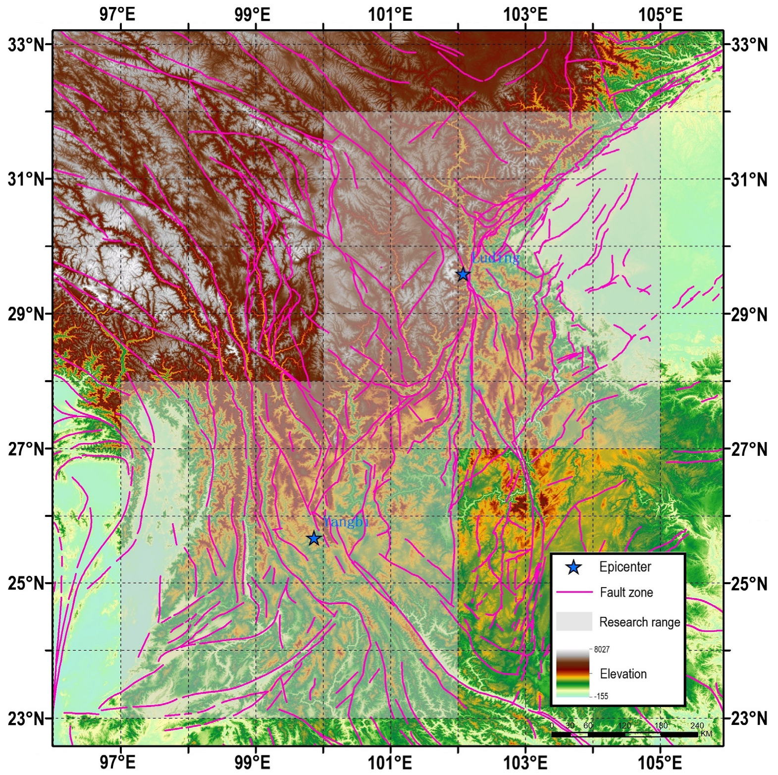
Figure 1. Research region. The pentagrams indicate the locations of epicenters, the gray area indicates the 5° × 5° study area, and the pink lines represent the fault zones.
Applsci 13 08572 g001
Figure 2. (a) OLR values in China in the 30 days before Yangbi Ms6.4 earthquake (from 22 April 2021 to 21 May 2021). The red box indicates the study area of the Yangbi earthquake. (b) The Yangbi Ms6.4 earthquake’s OLR values within the 5° × 5° range of the epicenter (from 22 April 2021 to 21 May 2021).
Applsci 13 08572 g002
Figure 3. Experimental flowchart. The experimental process is divided into four parts: Data Preparation, Algorithm Evaluation, Anomaly Extraction, and Result Analysis.
Applsci 13 08572 g003
Figure 4. LSTM unit structure diagram. h t 1 and h t are the hidden information of the previous cell output and this cell output, respectively; x t and y t are the input and output of this cell, respectively; C t 1 and C t are the cell states of the previous cell output and this cell output, respectively; f t , i t , and o t are the objective functions; σ is the sigmoid function.
Applsci 13 08572 g004
Figure 5. BILSTM structure diagram. x t and y t are the input and output of the model, respectively.
Applsci 13 08572 g005
Figure 6. Anomaly extraction method flowchart. The flowchart was modified based on the anomaly extraction method proposed by Zhai et al. [23] and Zhang et al. [50] in their articles.
Applsci 13 08572 g006
Figure 7. Prediction and anomaly performance of the 31.5° N 102.5° E grid OLR values of the Luding earthquake. The red curve is the predicted OLR value, and the blue and light blue curves are the upper and lower bounds of the confidence interval, respectively. The green curve is the actual OLR value; ΔOLR indicates how much the true value exceeds the prediction interval.
Applsci 13 08572 g007
Figure 8. Pre-earthquake OLR prediction and anomalies of the Yangbi Ms6.4 earthquake−spatial dimension.
Applsci 13 08572 g008
Figure 9. Pre-earthquake anomalies of the Yangbi Ms6.4 earthquake−temporal dimension. The X axis indicates the time, the Y axis indicates the grid position, and the Z axis indicates the degree of anomaly.
Applsci 13 08572 g009
Figure 10. Pre-earthquake OLR prediction and anomalies of the Luding Ms6.8 earthquake−spatial dimension.
Applsci 13 08572 g010
Figure 11. Pre-earthquake anomalies of the Luding Ms6.8 earthquake−temporal dimension. The X axis indicates the time, the Y axis indicates the grid position, and the Z axis indicates the degree of anomaly.
Applsci 13 08572 g011
Table 1. Detailed information of earthquake examples.
Time (UTC + 8)Longitude/° ELatitude /° NDepth/KMMagnitude/MSLocation
21 May 2021 21:4899.8725.6786.4Yangbi County, Yunnan Province
5 September 2022 12:52102.0829.59166.8Luding County, Sichuan Province
Table 2. Error results for different days and different grids points based on time series BILSTM prediction model.
BILSTM5 Days10 Days15 Days20 Days25 Days30 Days
23.5° N 97.5° E35.871444.460240.778844.053741.9544.4664
23.5° N 98.5° E21.1724.748526.765633.144533.242539.824
23.5° N 99.5° E24.107624.497530.206437.986837.929142.8743
23.5° N 100.5° E16.731418.934123.445242.108743.123941.4841
23.5° N 101.5° E31.099927.569531.994150.916149.846947.2746
24.5° N 97.5° E9.973424.958426.623633.599238.292436.2921
24.5° N 98.5° E13.388634.864635.285338.570637.17240.8611
24.5° N 99.5° E15.06525.625334.297140.879738.060440.7207
24.5° N 100.5° E15.052624.620227.086441.917742.583341.4012
24.5° N 101.5° E22.142526.937829.927544.082244.7342.7893
25.5° N 97.5° E42.691841.408838.959340.486443.869541.0631
25.5° N 98.5° E48.684639.993237.442639.502140.348941.4182
25.5° N 99.5° E22.45922.227629.177442.979539.947238.9058
25.5° N 100.5° E22.45922.227629.177442.979539.947238.9058
25.5° N 101.5° E23.254522.568130.591743.770644.070441.7547
26.5° N 97.5° E25.845326.504825.965232.77233.173631.2204
26.5° N 98.5° E42.686634.40631.359331.847634.024132.3093
26.5° N 99.5° E24.193725.33725.532632.00231.470730.8233
26.5° N 100.5° E12.957713.907525.165238.328837.100736.8696
26.5° N 101.5° E16.493319.150725.820638.298238.857637.6009
27.5° N 97.5° E16.310214.695619.924626.97434.203532.8196
27.5° N 98.5° E16.218913.548218.720728.045227.551826.2956
27.5° N 99.5° E42.154732.800829.784331.850430.741528.9882
27.5° N 100.5° E22.284830.657629.314632.400530.371429.3901
27.5° N 101.5° E35.995531.321231.209838.721735.233233.7072
Total RMSE619.292667.9708734.5553948.2177947.8418940.0596
Table 3. Total RMSE error of different time prediction models.
5 Days10 Days15 Days20 Days25 Days30 Days
ARMA625.0028647.0955835.6342871.0932882.8587941.6699
ARIMA718.1327738.40422060.74941034.04221542.7989928.8650
SVM775.9093784.3109806.06651025.37151034.86801026.3374
XGBoost640.0953670.1815773.8258930.6856964.0494946.3818
BILSTM619.2920667.9708734.5553948.2177947.8418940.0596
Disclaimer/Publisher’s Note: The statements, opinions and data contained in all publications are solely those of the individual author(s) and contributor(s) and not of MDPI and/or the editor(s). MDPI and/or the editor(s) disclaim responsibility for any injury to people or property resulting from any ideas, methods, instructions or products referred to in the content.