Artificial Neural Network for Indoor Localization Based on Progressive Subdivided Quadrant Method

Abstract

The exterior location of a user can be accurately determined using a global positioning system (GPS). However, accurately locating objects indoors poses challenges due to signal penetration limitations within buildings. In this study, an MLP with stochastic gradient descent (SGD) among artificial neural networks (ANNs) and signal strength indicator (RSSI) data received from a Zigbee sensor are used to estimate the indoor location of an object. Four fixed nodes (FNs) were placed at the corners of an unobstructed area measuring 3 m in both length and width. Within this designated space, mobile nodes (MNs) captured position data and received RSSI values from the nodes to establish a comprehensive database. To enhance the precision of our results, we used a data augmentation approach which effectively expanded the pool of selected cells. We also divided the area into sectors using an ANN to increase the estimation accuracy, focusing on selecting sectors that had measurements. To enhance both accuracy and computational speed in selecting coordinates, we used B-spline surface equations. This method, which is similar to using a lookup table, brought noticeable benefits: for indoor locations, the error margin decreased below the threshold of sensor hardware tolerance as the number of segmentation steps increased. By comparing our proposed deep learning methodology with the traditional fingerprinting technique that utilizes a progressive segmentation algorithm, we verified the accuracy and cost-effectiveness of our method. It is expected that this research will facilitate the development of practical indoor location-based services that can estimate accurate indoor locations with minimal data.

1. Introduction

Research on location-based services (LBS) for use in the home, industrial automation, and healthcare has seen increased interest because of the growth of the Internet of Things (IoT) [1].

Location estimation technology is increasingly important in the IoT service domain, especially in services like unmanned vehicles, intelligent transportation systems, and drones. Numerous services have been made available to enhance the convenience of individuals, and currently, location-based services are functioning effectively. Services known as LBSs give wireless network users pertinent information about a user’s location. A crucial element of LBSs that has been considered in the academic and industrial sectors is an accurate and affordable localization mechanism. The GPS technique has typically been used to resolve this problem in outdoor settings, but due to the obstruction, attenuation, or reflection of satellite signals in enclosed spaces, this method is not appropriate [2]. Finding a reliable and affordable indoor localization system is therefore a continuing issue in this field. LBSs are used in a variety of settings to accurately determine outdoor positions using GPS technology. These systems, however, encounter limitations when it comes to detecting signals indoors, making it challenging to estimate interior location. Various LBSs, including wireless personal area networks (WPAN) [3,4,5], wireless local area networks (WLAN) [4], and radio-frequency identification (RFID) [5], use words like dependability and distance to estimate interior locations. Wi-Fi is typically used in indoor location methods [6]. However, recent advancements in lighting, compactness, cheap cost, energy, and compatibility have spurred ongoing research on indoor WPAN sites, such as BLE and Zigbee [7]. The use of the received signal strength indicator (RSSI), which monitors the power level of the received signal, is a popular method in LBSs for completing tasks such as calculating robot placement in warehouses and tracking construction project personnel. Due to its low power consumption and sophisticated signal processing capabilities, RSSI-based location estimation technology has received a great deal of attention and has been thoroughly studied in the context of wireless sensor networks [2]. Additionally, the majority of wireless devices now come equipped with built-in RSSI circuits, eliminating the need for additional hardware and lowering the cost and power usage of the system.

The primary objective of this paper is to improve the precision of positioning in confined areas, specifically outperforming the transferrable sensor capabilities provided by IEEE 802.15.4 standard sensors in open spaces. Additionally, we investigate efficient methods for interpretating fluctuations in radio wave intensity emitted from stationary nodes, which exhibit a logarithmic decrease and are not directly correlated with distance. We use a multi-layer perceptron (MLP)-based technique using the B-spline curved equation to determine the final coordinates and to achieve more refined position tracking.

We propose a novel RSSI signal-based positioning system that utilizes RSSI subregionalization, neural networks, and B-spline methods to address the accuracy issues of the raw signals used in these studies.

2. Related Work

In traditional IEEE 802.15.4 signal-based indoor positioning systems, RSSI signals are always distorted by multipath effects. Yiu et al., in their research, investigated two factors: density of access points (APs) and the influence of using an outdated signature map. They proposed several approaches to generate a radio frequency distribution map [8].

Quadtree search and fractal direction entropy weighting (QSFDEW) is a brand new indoor fingerprint locating algorithm that was developed by Huang et al. [9]. This method incorporates the benefits of QSFDEW algorithms, improving the indoor location’s accuracy as well as speed. The QSFDEW algorithm’s implementation is an inventive method for enhancing indoor fingerprint locations.

A RSSI-based indoor locating system that uses a multilateration (MLT) technique for logistics applications was proposed by Wang et al. [10]. The authors used a sensor network for food transportation logistics and completed both simulations and live experiments. When six fixed nodes (FNs) were used, Wang et al. [10] showed that their system could deliver a localization error of less than 1 m. Additionally, tests using a module compliant with IEEE 802.15.4 revealed location errors of less than 1.8 m.

Previous studies, however, only take into account the accuracy of location estimation in a space where fixed nodes are placed close together while estimating the location by calculating the distance of RSSI signals in a vast space as a logarithmic function. The fingerprint method also has the drawback of requiring a full scan and learning the entire area’s location information.

A location system utilizing artificial neural networks (ANNs) was suggested in [11] as a solution to this issue. The research findings in [11] demonstrated that ANNs can greatly enhance localization performance in indoor contexts with multipath effects in a localization system based on Wi-Fi RSSI data. Further advancements are required due to the prediction uncertainty of ANNs, which can lower the trustworthiness of localization outcomes. Findings in [12,13,14,15] offer a deep neural network (DNN)-based localization system as a means of creating a more trustworthy localization system. In complex indoor environments, DNN-based localization systems have the capability to accurately determine and improve the positioning of objects or individuals. The primary challenges of DNN-based localization systems, however, are the training difficulties of DNNs and the need for a substantial amount of training data. A convolutional neural network (CNN) is suggested as an alternative to enhance localization performance in [16]. CNN-based localization techniques deliver precise building and floor predictions using RSSI time series from WLAN access points. A CNN-based localization system can be implemented with few resources, but it is challenging because of the memory required for activation at the network layer.

For localization systems based on Wi-Fi RSSI signal, a novel time series semi-supervised learning technique is proposed in [17]. Compared to the current Wi-Fi RSSI signal-based localization method, the semi-supervised learning algorithm produces results for locations that are more accurate. The extreme learning machine (ELM) [18] that is described in this study is used in a Wi-Fi positioning system to lessen the effort required to calibrate Wi-Fi fingerprint maps. The Wi-Fi fingerprint maps are created more quickly and with less labor due to the ELM’s quick learning rates, which also enhance the performance of localization. But in terms of precision and accuracy, the localization outcomes of ELM-based systems can fall short of deep learning-based systems [19]. Recurrent neural networks (RNN) and long short-term memory (LSTM) models are used to create localization systems in [20,21,22]. Additionally, [23] provides a Wi-Fi indoor localization system based on deep learning models that surpasses the current Wi-Fi RSSI signal-based localization system. This system uses RSSI and channel state information (CSI).

To solve the challenge of RSSI signals, [24] suggested a Wi-Fi RSSI signal-based positioning system that employs RSSI heat maps rather than RSSI raw values. However, these deep learning model-based positioning systems use raw RSSI data from APs to perform positioning. According to experimental findings, among all current deep learning techniques, the proposed Wi-Fi RSSI heat map-based positioning system using HDLM offers the best positioning accuracy.

The primary objective of this paper is to improve the precision of positioning in confined areas, specifically outperforming the transferrable sensor capabilities provided by IEEE 802.15.4 standard sensors in open spaces. Additionally, we investigate efficient methods for interpretating fluctuations in radio wave intensity emitted from stationary nodes, which exhibit a logarithmic decrease and are not directly correlated with distance. We use a multi-layer perceptron (MLP)-based technique using the B-spline curved equation to determine the final coordinates and achieve more refined position tracking.

The remainder of this paper is organized as follows. Section 3 provides a detailed explanation of an indoor location system that utilizes the MLT mechanism based on the RSSI measurements. In Section 4, the proposed strategy is elaborated upon. The experimental design and findings, as well as any relevant discussion, are presented in Section 5 and Section 6, respectively. Finally, Section 7 offers an overview of the study’s findings.

3. RSSI Signal Based MLT Location Estimation

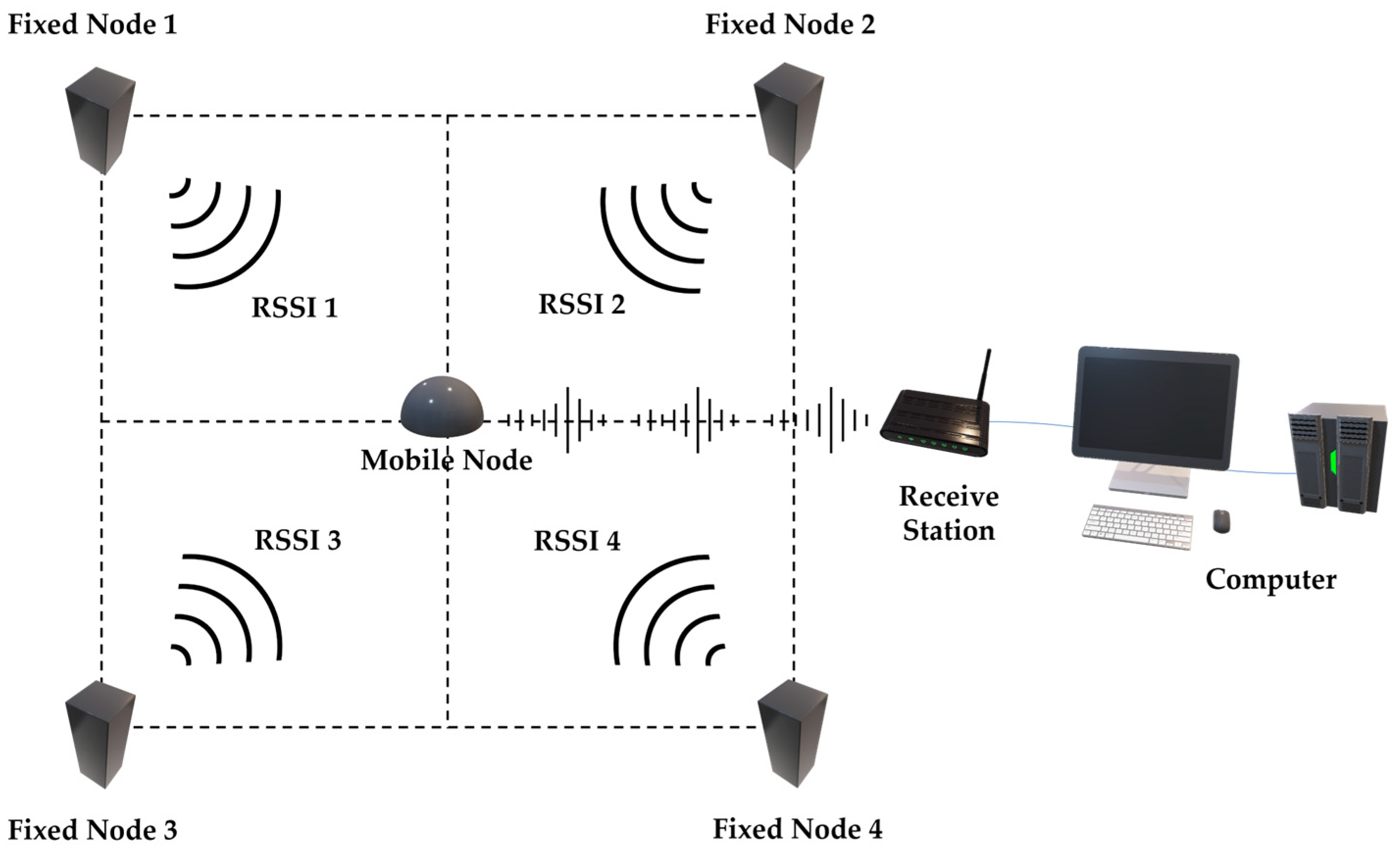
Figure 1 depicts the WSN system employed in this investigation. More fixed nodes will produce more reliable data, but they will also increase the cost and complexity of the system. To select location coordinates in a rectangular-shaped range, we chose four nodes, which is a simple and minimal number [1,2,6]. At the predetermined positions, there were four fixed nodes (FNs): FNs 1 (0, 3), 2 (3, 3), 3 (0, 0), and 4 (3, 0). The computational and receiving components of the system were combined into a receive station node (RSN). Within the restricted area, a mobile node (MN) of unknown identity was located. The FNs, which were situated at predefined points, sent RSSI signals to the MN. A mathematical equation based on the information received by the MN was used to estimate the MN’s coordinates. We developed an indoor positioning system based on RSSI. It consists of three steps: gathering the RSSI measurements using a communication protocol that has been designed, converting the RSSI measurements into distances using a PLE, and using a multi-signal algorithm.

3.1. RSSI Measurement and Acquisition

A network made up of all the nodes was created to find the MNs. A beacon packet was created by the RSN and sent to the MN. After receiving the packet, the MN gathered the FN ID, location, and packet number from it while measuring the FN’s RSSI readings. Additionally, the MN sent a report packet containing the data it had gathered to the RSN, which then sent it on to the computer. Using the identity, RSSI, and values, location, and packet number of each FN, the MN’s position was ascertained.

3.2. Transformation to RSSI Values to Distances

A computer used PLE to convert the RSSI values from all FNs into distance values [25]. This equation states that the distance calculated in a 3 × 3 m examination area can be used to calculate the RSSI. Equations (1) and (2), which calculate the average RSSI in dBm based on the relationship between the ${RSSI}_i$ and the associated distance, show the PLE. At a reference distance from the ${RSSI}_i$ transmitter, the average RSSI (dBm) is calculated [25]. The path-loss index, denoted by the symbol k, displays the rate of signal loss as a function of distance. After gathering RSSI readings from a test field where the separation between the transmitter and receiver was known, the ${RSSI}_i$ were calculated.

$${RSSI}_i\left(dBm\right)={RSSI}_{i_0}\left(dBm\right)-\left.\left[10\times k\times {\log }_{10}\frac{d}{d_0}\right.\right]$$

(1)

$$d={10}^{\frac{RSS{I}_{i_0}\left(dBm\right)-RSS{I}_i\left(dBm\right)}{10\times k}}, for d_0=1$$

(2)

4. Proposed Methods

As mentioned in [26,27,28,29,30,31,32,33], RSSI signals tend to exhibit low repeatability as they vary over time. They change with time for a variety of reasons, including the hardware used, the distance between the transmitter and receiver, the measurement period, the interference from external devices, the presence and movement of people, and the surrounding environment (the type of building, any obstructions, and the materials used) [33].

Conventional MLT methods frequently result in estimated locations that fall outside the defined test area, as demonstrated in previous studies [10,33]. To overcome this issue, we utilized an ANN method that relies on converted distances and RSSI signals to estimate location. Additionally, we employed a refined location estimation approach based on a progressive subdivided quadrant method, allowing us to improve the accuracy of our localization system. 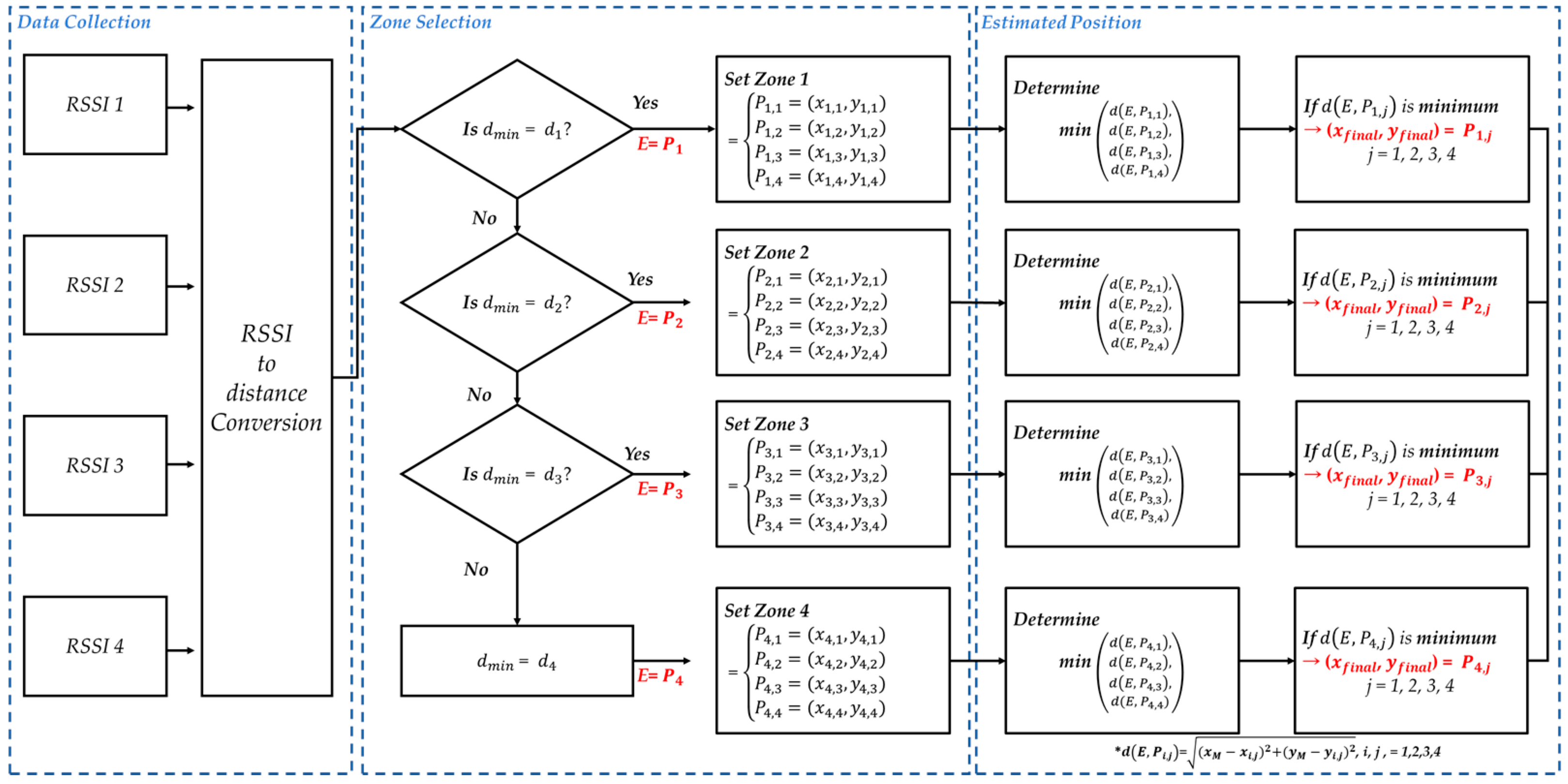Figure 2 illustrates the proposed system.

Three processes make up the suggested system in Figure 2: (a) zone generation using PSQ, (b) zone selection, (c) and estimation of location using the B-spline surface equation. The following is a detailed description of the steps.

Traditional supervised deep neural networks often have both offline and online phases for localization. An extensive dataset, made up of measurable data split into training and validation sets, is used to build and validate a model during the offline phase. In this instance, the ANN model applies the data directly without preprocessing by using received signal strength indicator (RSSI) values gathered from nine ground truth locations as inputs and producing the appropriate user location information. The ANN model can precisely pinpoint a mobile node using the training dataset once it has been optimized. To achieve high localization accuracy, it is necessary to gather a sizeable number of dense, labeled data samples, but doing so is expensive and time-consuming. To address this issue, we segment the data into zones (regions) and create high-resolution data labels, and then apply neural network learning to them.

In this study, we offer a method for generating artificial data that complements genuine labeled acquisition data using a progressive segmentation methodology. To accomplish location prediction, the algorithm blends actual gathered data with artificially increased data. Furthermore, to ensure consistent data quality and coordinate prediction, the system converts the distance measurement to an equivalent FN value.

For localization, actual data are merged with the generated signal’s magnitude and translated distance. FNs and MNs were used in the experiment, which took place in a 3 × 3 m indoor area. RSSI signals were recorded for each access point. The online location region prediction is then performed using the learned ANN model. Based on the generated data, a region is chosen, and the B-spline curve equation is applied to estimate its location. The suggested framework employs B-spline approaches and progressive segmentation techniques to efficiently estimate the location of mobile nodes in a 3 × 3 m interior environment with little data collection.

4.1. Proposed Method for Virtual Data Generation Using PSQ

The received signal strength indicator value obtained at a fixed node (FN) is divided into log scales using the suggested incremental segmentation method to produce a virtual coordinate of the mobile node (MN). By limiting the amount of labeled training data, PSQ-based localization aims to solve the costs and difficulties of acquiring labeled data while perhaps avoiding overfitting issues that could arise with deep learning-based localization. In order to enhance the effectiveness of supervised learning, these technologies make use of both created and acquired data.

In a segmentation and conquest strategy, a given problem is divided into two or more subproblems, which are typically taken directly from the original problem. It is possible to segment subproblems into smaller ones or use the solutions to a segmented subproblem directly to calculate solutions to a given problem. This method divides small cases into smaller ones until a solution is found. The segmentation and conquering algorithm uses a top-down methodology in which answers to the child problem are used to calculate answers to the parent problem.

In this study, the log scale of the RSSI signal was gradually divided using a threshold determination technique to produce data for the center values at 25 points and 16 zones on the 5 × 5 grid. A conceptual diagram of the PSQ algorithm employed in this study is shown in Figure 3. For the binary segmentation process to create four node values and intermediate values in the segmented zone, a 3 m × 3 m space must be divided into four 1.5 m × 1.5 m intervals.

To estimate the coordinates of $(x_e, y_e)$ for PSQ, one zone is divided into four regions. If each x-coordinate is from $x_0$ to $x_1$ and the y-coordinate is from $y_0$ to ${ y}_1$, it is divided into four zones (Zones 1 to 4), each of which is defined in the same way as Equation (3). The symbols used in this study are shown in

Table 1. Symbols used in the study.

Symbols	Definition
$x_{\mathrm{0,1}}$	x-coordinate of the fixed node
$y_{\mathrm{0,1}}$	y-coordinate of the fixed node
$(x_e, y_e)$	$\mathrm{Expected} \mathrm{coordinates} \mathrm{of} (x, y)$
$\left[Q\right]$	Curve equation in matrix form
$\left[B\right]$	Control points coordinate
$\left[E^k\right]$	Error of the kth value
${\left[B\right]}^{\prime }$	Converted control point matrix
${\left[T\right]}_k$	Translation matrix of the selected cell k.
$(u_e, v_e)$	$\mathrm{Expected} \mathrm{parametric} \mathrm{values} \mathrm{of} (u, v)$
$(x_m, y_m)$	Converting coordinates form RSSI

.

$$\left\{\begin{array}{c}Zone 1:\left(x_0\le x\le \frac{x_1 + x_0}{2}\right), \left(\frac{y_1 + y_0}{2}\le x\le y_1\right)\\ Zone 2:\left(\frac{x_1 + x_0}{2}\le x\le x_1\right), \left(\frac{y_1 + y_0}{2}\le x\le y_1\right)\\ Zone 3:\left(x_0\le x\le \frac{x_1 + x_0}{2}\right), \left(y_0\le x\le \frac{y_1 + y_0}{2}\right)\\ Zone 4:\left(\frac{x_1 + x_0}{2}\le x\le x_1\right), \left(y_0\le x\le \frac{y_1 + y_0}{2}\right)\end{array}\right.$$

(3)

The measured area was divided into 4 zones, as depicted in Figure 4, and 4 subdivided cells were chosen as selection regions.

4.2. Zone Selection-Based ANNs

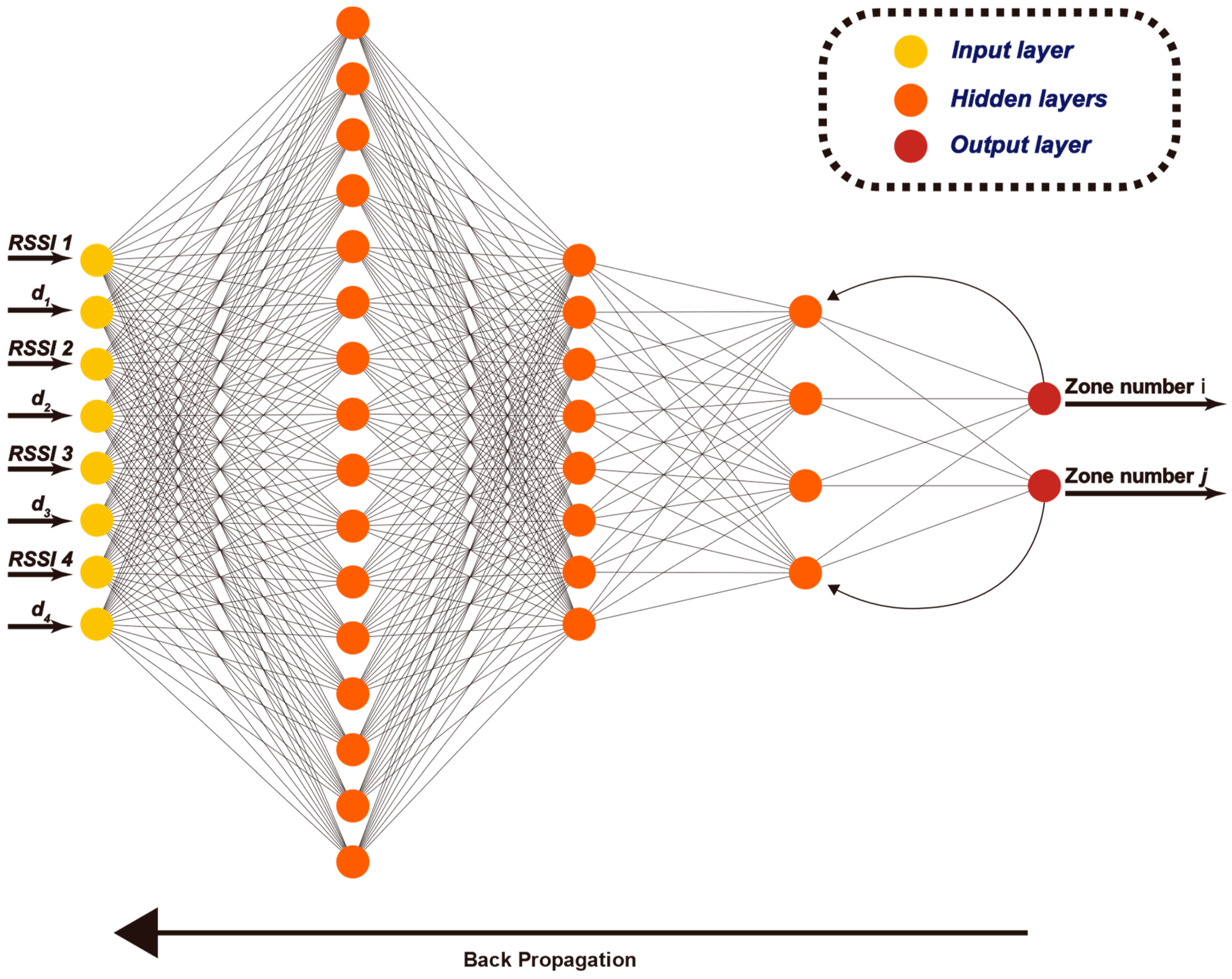
ANNs are made up of multilayered structures. Multi-layer perceptron (MLP) is the approach that artificial neural networks most frequently utilize to approximate functions. Figure 5 depicts the MLP’s structural layout.

MLP consists of input layers, hidden layers, and output layers, as shown in Figure 5. A typical MLP usually has multiple nodes connecting it. The network structure must first be established before building an artificial neural network. The computation of the solution only requires one hidden layer if the input nodes can be linearly separated. Finding the optimal solution is difficult in situations with eight input nodes, like the one described in this study. In this study, we built an artificial neural network training model using stochastic gradient descent (SGD) among backpropagation algorithms. SGD is a variant of gradient descent that uses minibatches, or just one data point, to calculate the error and update the weights. By dividing the data to be calculated into small batches, memory is efficiently used. Backpropagation algorithms like these show significant differences in learning effectiveness and predictive power depending on the number of hidden layers and nodes.

The maximum number of learning iterations was set at 1000 to enable the determination of the ideal artificial neural network topology. The number of hidden layers was set to three, the output layer node to two, and the input layer node to eight. There were 16 nodes in the first hidden layer, 8 nodes in the second, and 4 nodes in the third hidden layer. The logarithmic sigmoid function was employed as the activation function in the hidden layers. The input layer was composed of virtual region labeling data that included node signals from the 16 virtual regions and the four fixed nodes.

Results are output through the three hidden layers and two output layers. The output value was selected in four rows and four columns $(i,j)$ and was represented by zone selection in 16 cases. Because the weight changes in neural network learning were taken randomly, the results differed, and the number of attempts varied each time. Thus, the generation seed was fixed, and the optimal method and loss function were selected for learning. The model obtained the optimum MSE (highest) value using the Adam optimization method and a sequential network comprising five dense layers. The loss function for polynomial classification was defined as binary cross-entropy, while the performance evaluation was influenced by accuracy. The fitting method was used to carry out the learning process as with other neural networks, and callback functions were employed to prevent overfitting. To ensure the lowest loss feasible, the training process was stopped if the validation loss increased three times in a row. The learning model’s findings were verified using the average squared error (MSE, mean squared error) and the coefficient of determination.

The mean squared error (MSE) and coefficient of determination $R^2$ were used to evaluate the performance of the learning model [33]. MSE is a statistic for evaluating the learning effectiveness of ANNs. A more reliable model is one that has a lower MSE value. R2 estimates the percentage of the dependent variable’s variability that can be predicted from the independent variables. The value $R^2$ = 1 shows that all sample observations lie on the estimated regression line, and the closer the value is to 1, the better the fit. To evaluate the learning outcomes, 60, 20, and 20% of the total learning data were randomly assigned for training, validation, and testing, respectively.

The SGD optimization model and a sequential network with five dense layers, as previously reported [34], were used to produce the optimum MSE (best value). While accuracy affects performance evaluation, binary cross-entropy is the definition of the loss function for polynomial classification. Similar to other neural networks, the fitting approach was used for training, with the callback function being used to avoid overfitting. To achieve the lowest loss feasible, the training procedure was stopped when the validation loss increased consecutively three times or more.

The proposed method employs the database values of $d_1$ to $d_4$ to predict the expected location of the unidentified MN as zone number. The development of an ANN requires prior definition of its network structure. The inputs into the neural network comprise the RSSI signal values and RSSI-to-distance transformation, represented by ($d_1$, $d_2$, $d_3$, $d_4$, RSSI1, RSSI2, RSSI3, RSSI4). This study showed that, when there are eight input nodes, the optimal regression value cannot be determined using a single hidden layer [33].

A neural network Is created by increasing the coefficient of the hidden layer to solve this issue. The results of the proposed algorithm show that the number of hidden layers and nodes makes a significant difference in learning effectiveness and forecasting capability [33].

The curve fitting method chooses coordinates to approximate the precise location in the cell after an area has been defined. By replacing the B-spline curved expression for a formula provided by the chosen parameter value and utilizing it as a look-up table, one of the methods for choosing coordinates can be utilized to choose a position.

4.3. Estimated Location Compensation Using B-Spline Surface Equation

When a potential area is chosen, the coordinates are derived by applying the B-spline curved expression in the standard cell to calculate the parameters u and v. Standardized and numbered from 0 to 1, the u and v parameters are used to calculate coordinate values by transforming them into particular cells. Using curved equations in two dimensions in selected cells, such as employing LUTs, has been suggested to monitor the location. Since data must be compared and cell locations must be computed using linear proportional equations, tracking locations with LUTs is laborious. B-spline surface equation data can be saved as a surface and utilized in place of LUTs to resolve this issue. The equation for the B-spline surface is as follows:

$$Q\left(u, v\right)={\sum }_{i=0}^m{\sum }_{j=0}^n{B}_{i,j}{S}_{i,j}(u, v)$$

(4)

$B_{i,j}$ represents the control points of B-spline equation, and $S_{i,j}$ is the basis function for parameters u and v. This surface equation can be represented in matrix form as follows:

$$\left[Q\right]=\left[S\right]\left[B\right]$$

(5)

The node coordinate value $\left[Q\right]$ is represented in this curve equation. Control point coordinate $\left[B\right]$ computed coordinates are as follows when using Equation (6):

$$\left[B\right]={\left[S\right]}^{-1}\left[Q\right]$$

(6)

If the data was generated using a rectangular polygon net of dimensions $m\times n$, the matrix [D] can be represented as $m\times n\times 2$, effectively removing the height variable equation on the 3-D coordinate axis. To solve the problem, an ideal algorithm must be used. The control point acts as the interpolation, making sure that each data coordinate on the surface of the curve is traversed. Each node must be supplied with the variable parameters u and v in order to acquire interpolation data using the provided data coordinates. The two variable parameters u and v have an acceptable range that is determined by:

$$0\le u\le 1.0, 0\le v\le 1.0$$

(7)

To perform curve interpolation and ensure the calculation of the control point $B_{i,j}$, it is necessary to meet the requirements of the following equation:

$$E_{i,j}^{k+1}=E_{i,j}^k+\left(Q_{i,j}-{\sum }_{i=0}^m{\sum }_{j=0}^n{B}_{i,j}{S}_{i,j}(u, v)\right)$$

(8)

The control value of $E_{i,j}^k$ is the error of the kth value in solving the equation. The operation is repeated until the error value is below the given common difference. The disparities between data that has been measured and calculated make up the objective function. In the B-spline curved expression, the control point $\left[B\right]$ is converted into the selected cell as follows:

$${\left[B\right]}^{\prime }={\left[T\right]}_k\left[B\right]$$

(9)

Here, ${\left[B\right]}^{\prime }$ is the converted control point matrix, and ${\left[T\right]}_k$ is the moving translation matrix of the selected cell k.

In the given B-spline Equation (6), the expecting $(u_e, v_e)$ value may be calculated as follows:

$$({\mathrm{x}}_e, {\mathrm{y}}_e)={\sum }_{i=0}^m{\sum }_{j=0}^n{B\prime }_{i,j}{S}_{i,j}(u_e, v_e)$$

(10)

$$u_e=\frac{x_m-x_0}{x_1-x_0}$$

(11)

$$u_e, v_e=0 if u, v<0 and u_e, v_e=1 if u, v>1$$

(12)

Here, $x_m$ and $y_m$ are values obtained by converting RSSI signals received from four FNs into distances. If each x-coordinate ranges from $x_0$ to $x_1$ and the y-coordinate ranges from $y_0$ to $y_1$, it is divided into four zones (Zones 1 to 4). These divisions are determined based on RSSI signals received from the four FNs that have been converted into coordinate values of $x_m$and $y_m$. The $x$ coordinates are $x_0$ to $x_1$and the y coordinates are $y_0$ to $y_1$. Within the divided area, the $(x_e, y_e)$coordinates are calculated by $u_e,v_e$parameters.

5. Experimental Environment

The experiment was conducted at the Industrial Engineering Lab, Room 312, Engineering Building, Cheonan Campus, Dankook University, Republic of Korea.

In the laboratory, an RSSI-based location system was built in one-third of the room. The measurement area was 3.0 × 3.0 m, as shown in Figure 5. The area where the wireless network was established was empty, whereas the experiment was conducted in a workspace with office equipment and a PC set up in the remaining area.

In this study, a Zigbee wireless network protocol was utilized. The Zigbee wireless sensor was established on the physical layer of IEEE 802.15.4 standard’s low-rate wireless personal area network (LR-WPAN) communication [7,35]. An XBee module, a commonly used product, was employed, and the network was configured by assigning a coordinator, router, and end device. To mitigate interference, channel 20 was established as the frequency of the XBee S2C sensor because it was in a different frequency band from the prevalent 2.4 GHz Wi-Fi in buildings [2].

In the XBee S2C sensor, each FN is subordinate to the MN, which transmits signals. Signal flow was set to occur in only one direction. The Arduino Mega 2560(Arduino SRL, Via Andrea Appiani 25, 20900 Monza MB) controller in the MN, which served as a router, read the RSSI values of the four FNs and transferred the received values to the RSN.

Four FNs were anchored to one of the four corners: (x₁ = 0.00, y₁ = 0.00), (x₂ = 3.00, y₂ = 0.00), (x₃ = 3.00, y₃ = 3.00), and (x₄ = 0.00, y₄ = 3.00). We ensured that all nodes were 1.2 m above ground, with a 3 m distance between FNs, to avoid various radio-wave interferences, such as diffraction and reflection from the floor, as shown in Figure 5. Measurements were conducted using a tripod to maintain similar variables that may occur between experiments, such as accurate measurements from the device and the state of the device. Signals received from the four FNs to the MN were sent to a computer to estimate the MN’s location.

Table 2. Virtual Locations for the Experiment.

Virtual Locations: Experiment
Zone 1 = (0.75, 2.25)		Zone 2 = (2.25, 2.25)
$P_{1,1}$ $P_{1,2}$ $P_{1,3}$ $P_{1,4}$	$(x_{1,1}, y_{1,1})=(0.375,2.625)$ $\left(x_{1,2}, y_{1,2}\right)=\left(1.125,2.625\right)$ $(x_{1,3}, y_{1,3})=(0.375,1.875)$ $\left(x_{1,4}, y_{1,4}\right)=\left(1.125,1.875\right)$	$P_{2,1}$ $P_{2,2}$ $P_{2,3}$ $P_{2,4}$	$(x_{2,1}, y_{2,1})=(1.875,2.625)$ $\left(x_{2,2}, y_{2,2}\right)=\left(2.625,2.625\right)$ $(x_{2,3}, y_{2,3})=(1.875,1.875)$ $\left(x_{2,4}, y_{2,4}\right)=\left(2.625,1.875\right)$
Zone 3 = (0.75, 0.75)		Zone 4 = (2.25, 0.75)
$P_{3,1}$ $P_{3,2}$ $P_{3,3}$ $P_{3,4}$	$(x_{3,1}, y_{3,1})=(0.375,1.125)$ $\left(x_{3,2}, y_{3,2}\right)=\left(1.125,1.125\right)$ $(x_{3,3}, y_{3,3})=(0.375,0.375)$ $\left(x_{3,4}, y_{3,4}\right)=\left(1.125,0.375\right)$	$P_{4,1}$ $P_{4,2}$ $P_{4,3}$ $P_{4,4}$	$(x_{4,1}, y_{4,1})=(1.875,1.125)$ $\left(x_{4,2}, y_{4,2}\right)=\left(2.625,1.125\right)$ $(x_{4,3}, y_{4,3})=(1.875,0.375)$ $\left(x_{4,4}, y_{4,4}\right)=\left(2.625,0.375\right)$

lists the compensated locations established in Section 3 for each zone of the proposed test field. As discussed in the previous section, additional segmentation processes can be employed to improve estimation accuracy. However, the scale of the network influences this, increasing computational complexity. Hence, obtaining an optimal segmentation step is difficult and requires further study.

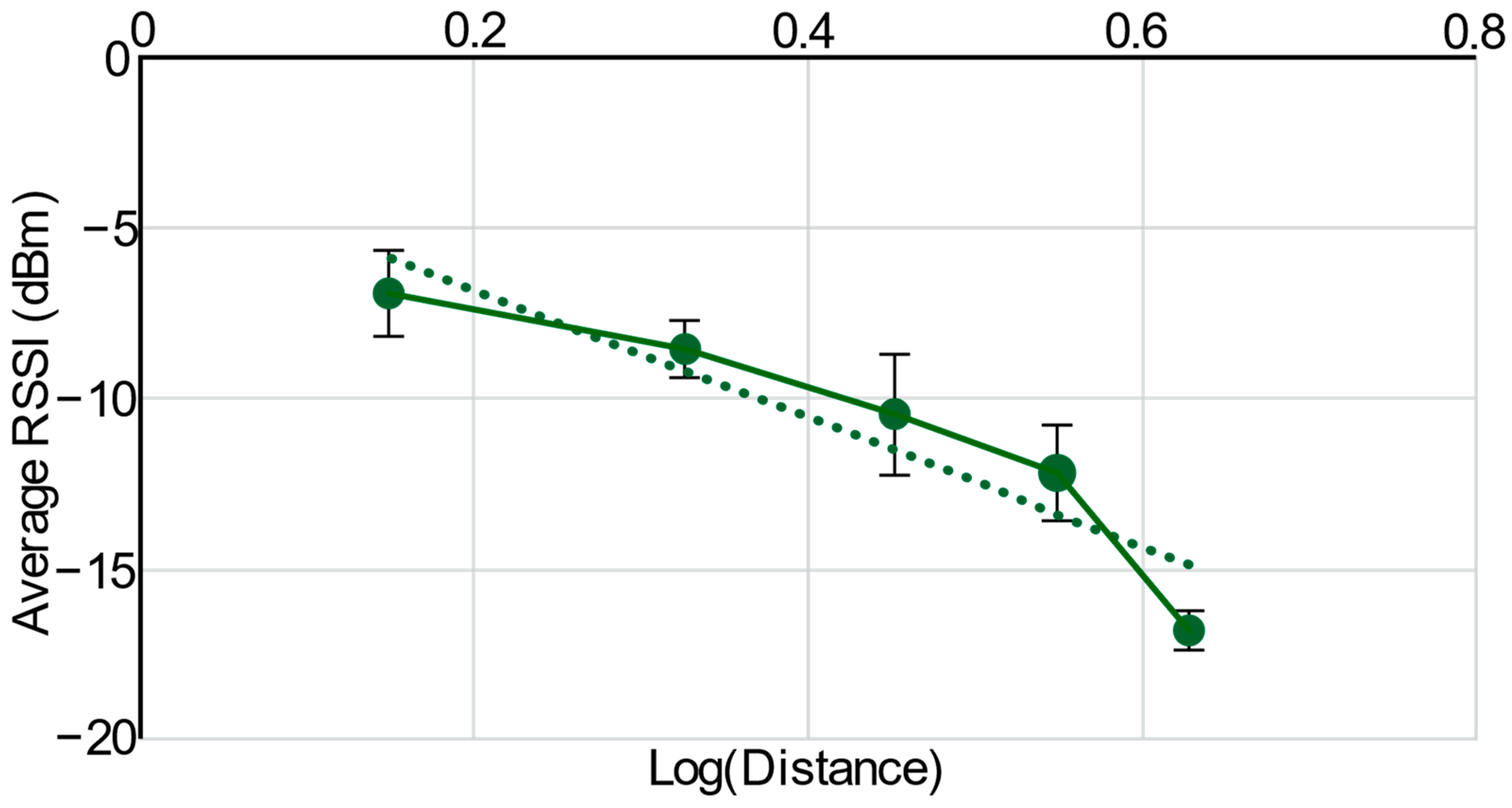
As explained in Section 2, the RSSI was transformed into a distance measure for the indoor location using PLE. The methodology for estimating the PLE in the test field includes monitoring the RSSI data at various distances using a single transmitter and an RSN. In the test field, the receiver collected 8000 samples of the RSSI data at different distances from each FNs. Figure 6 shows the resulting data as a logarithmic plot of the average RSSI in dBm versus distance in meters. The experimental PLE for the environment was calculated using linear regression analysis.

6. Results and Discussion

Metrics and Evaluation of Performance

Python was used to create deep learning models, along with libraries like TensorFlow 2. Three measures—MSE, root MSE (RMSE), and mean absolute error (MAE)—were used to calculate the difference between the estimated location and the actual value in order to evaluate the model’s performance. According to Section 4, the localization error and prediction accuracy of the model on the datasets were assessed. By averaging the absolute values of the errors, MAE was calculated.

$$MAE=\frac{1}{n}{\sum }_{i=1}^n|P{S}_i-S{A}_i|$$

(13)

According to Equation (14), MSE is the average of the squared differences between the estimated and actual values. The average size of the prediction mistakes is shown by the following equation:

$$MSE=\frac{1}{n}{\sum }_{i=1}^{\mathsf{\Pi }}{(P{S}_i-S{A}_i)}^2$$

(14)

The average difference between the expected and actual values is quantified by the statistic known as RMSE, which can be used to assess the accuracy of a model’s predictions. This value gives a thorough evaluation of the model’s performance and is obtained by calculating the square root of the residual. In several domains, RMSE is frequently used to evaluate the difference between expected and actual results.

$$RMSE=\sqrt{\frac{{\sum }_{i=1}^n{(P{S}_i-S{A}_i)}^2}{n}}$$

(15)

The number of experiments performed is represented by n in the equation. The prediction of the final location by the proposed algorithm is denoted as $P{S}_i$, while the actual final location in the i-th experiment is referred to as $S{A}_i$. The performance of the best-fitting model was evaluated by incorporating batch normalization into the MLP regression algorithm and analyzing the impact of various numbers of hidden layers. The accuracy of the model predictions was determined by computing the ratio of the correct predictions to the total predictions. The optimization process was performed using the Adam optimizer, and all activation functions were performed using it. The results indicated that the SELU activation function had a lower location error (0.65 m compared to the other activation functions (ReLU, Softplus, and ELU)), thus demonstrating its superior performance.

The decay curves of the loss function for various epochs of the training and validation datasets are shown in Figure 7. The stability of the curve was observed after 60 epochs, but the observations were extended to 140 epochs for further confirmation of the results.

The proposed model was used to determine the quadrants in sequential steps and the error distance for the target coordinates. The results of this analysis are presented in

Table 3. Experimental results after the first step of the PSQ method.

Target Coordinates	1 Step of Quadrant	Estimated Coordinates	Error Distance
(0, 3)	0.0006, 0.0024	(0.75, 2.25)	1.06 m
(1, 3)	0.0087, 0.0170		0.79 m
(0, 2)	0.0331, 0.0046		0.79 m
(1, 2)	0.0998, 0.0020		0.35 m

and

Table 4. Experiment results after the second step of the PSQ method.

Target Coordinates	2 Step of Quadrant	Estimated Coordinates	Error Distance
(0, 3)	0.0002, 0.0018	(0.38, 2.63)	0.53 m
(1, 3)	0.0013, 0.9650	(1.13, 2.63)	0.40 m
(0, 2)	1.0000, 0.0000	(0.38, 1.88)	0.40 m
(1, 2)	0.9974, 0.9976	(1.13, 1.88)	0.18 m

, respectively. These tables provide a comprehensive summary of the proposed model’s performance and its ability to accurately predict the target coordinates.

The results obtained from the proposed model exhibit a remarkable level of accuracy in predictions, with the lowest location error being 0.18 m. The largest recorded location error was 1.06 m, which exceeded the performance of the sensor. These results demonstrate the capability of the proposed model to precisely forecast the target coordinates.

The average error distance determined using the MLT approach was 1.603 m, according to Figure 8. In contrast, the proposed methodology has a much lower average error of 0.5625 m. These findings demonstrate that the proposed approach outperforms existing MLT methods.

7. Conclusions

In this work, we have developed a system that addresses the challenge of accurately estimating indoor environments by utilizing RSSI readings from four FNs.

We used tracking system approaches based on RSSI to create precise internal positions. We discovered that employing signal averaging techniques and fingerprinting approaches helped accuracy to some degree. However, it was noted that errors still persisted when dealing with weak signals, especially in corners of the area, leading to poor performance across the entire region. The fingerprinting method entailed significant expenditures due to the considerable data collection needed to cover a large area.

We suggested using B-spline fitting methods and artificial neural network (ANN) approaches to identify the final location in order to overcome this problem. The study showed that the proposed strategy may achieve location learning with only a small amount of data-by-data augmentation. The target region was gradually divided using this method, which was based on the ANN method and used signal analysis and domain segmentation to precisely track the moving node’s location.

Instead of using lookup tables (LUTs), we approximated the B-spline surface. This approach produced more accurate coordinate values compared to fingerprinting methods.

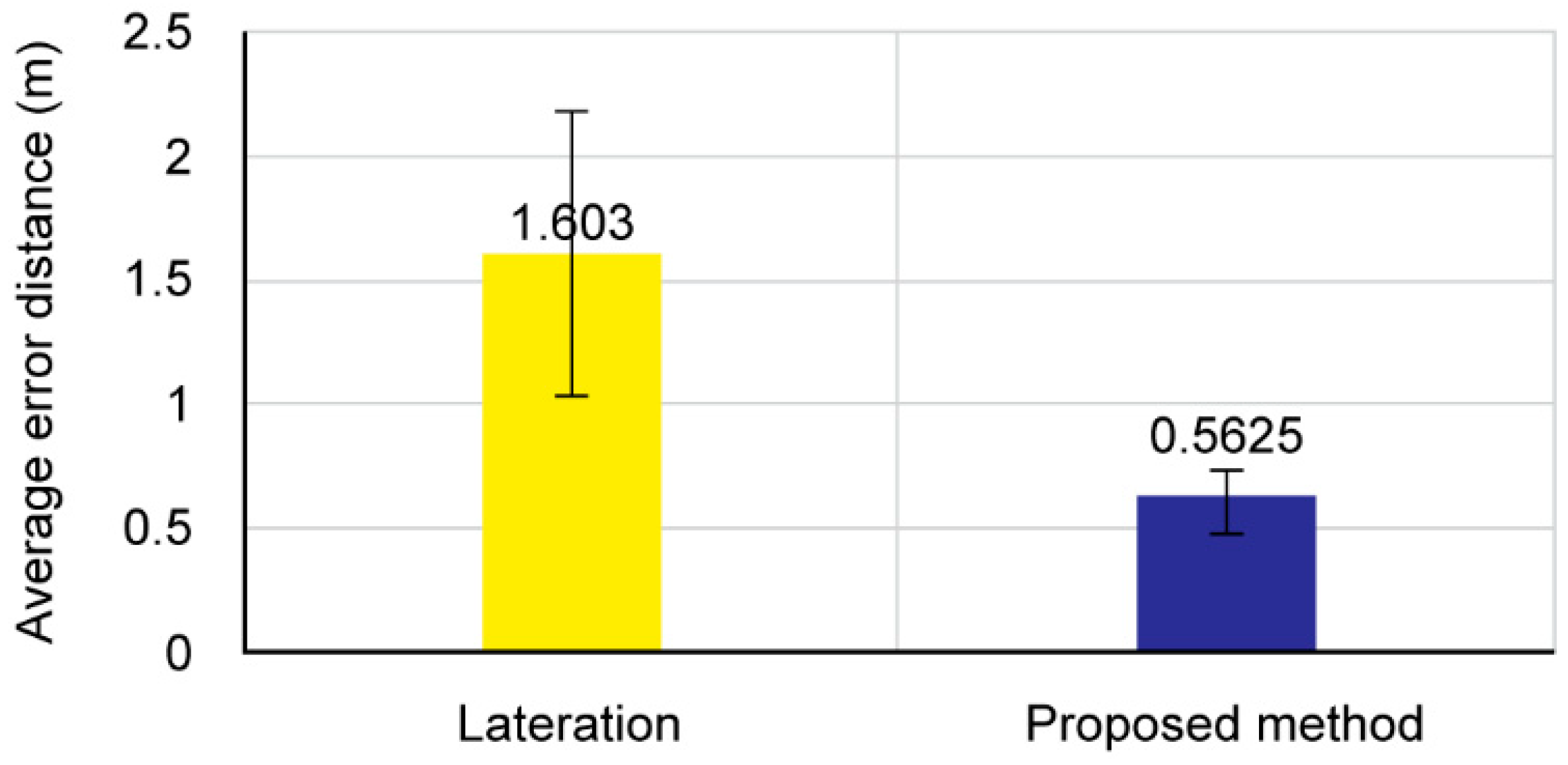
Our proposed model has shown an impressive level of prediction accuracy, as evidenced by the lowest reported position error of 0.18 m. Although there were instances where the sensor’s limits were exceeded by the highest position inaccuracy, resulting in 1.06 m, overall, the results demonstrate how well our suggested model can predict target coordinates.

The suggested method’s adaptability allows for its application in various scenarios, including indoor activities to identify target locations in unrestricted open spaces. Moreover, the internal location tracking system we developed can also be adapted for uses such as portable robots, automated guided vehicles (AGVs), and mobile phones (LBS). However, it may be more difficult to find the optimal weights when the signals have shorter intervals, and accuracy may suffer when fewer location signals are collected than now.

In our future research, we aim to enhance the accuracy of the location estimation system by investigating the optimal number of quadrant steps while taking into computational the computational time complexity. In addition, we can extend the application of our PSQ algorithm to outdoor localization by combining RSSI signals and time-series deep learning algorithms as in [36,37,38] for precise localization within the cell of an external base station.