
Estimation of Methane Gas Production in Turkey Using Machine Learning Methods

 , , , , and
Abstract
1. Introduction
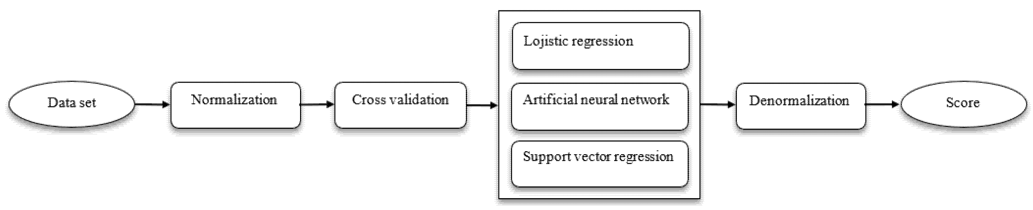
2. Materials and Methods
2.1. Data Set
2.2. Machine Learning
2.2.1. Logistic Regression
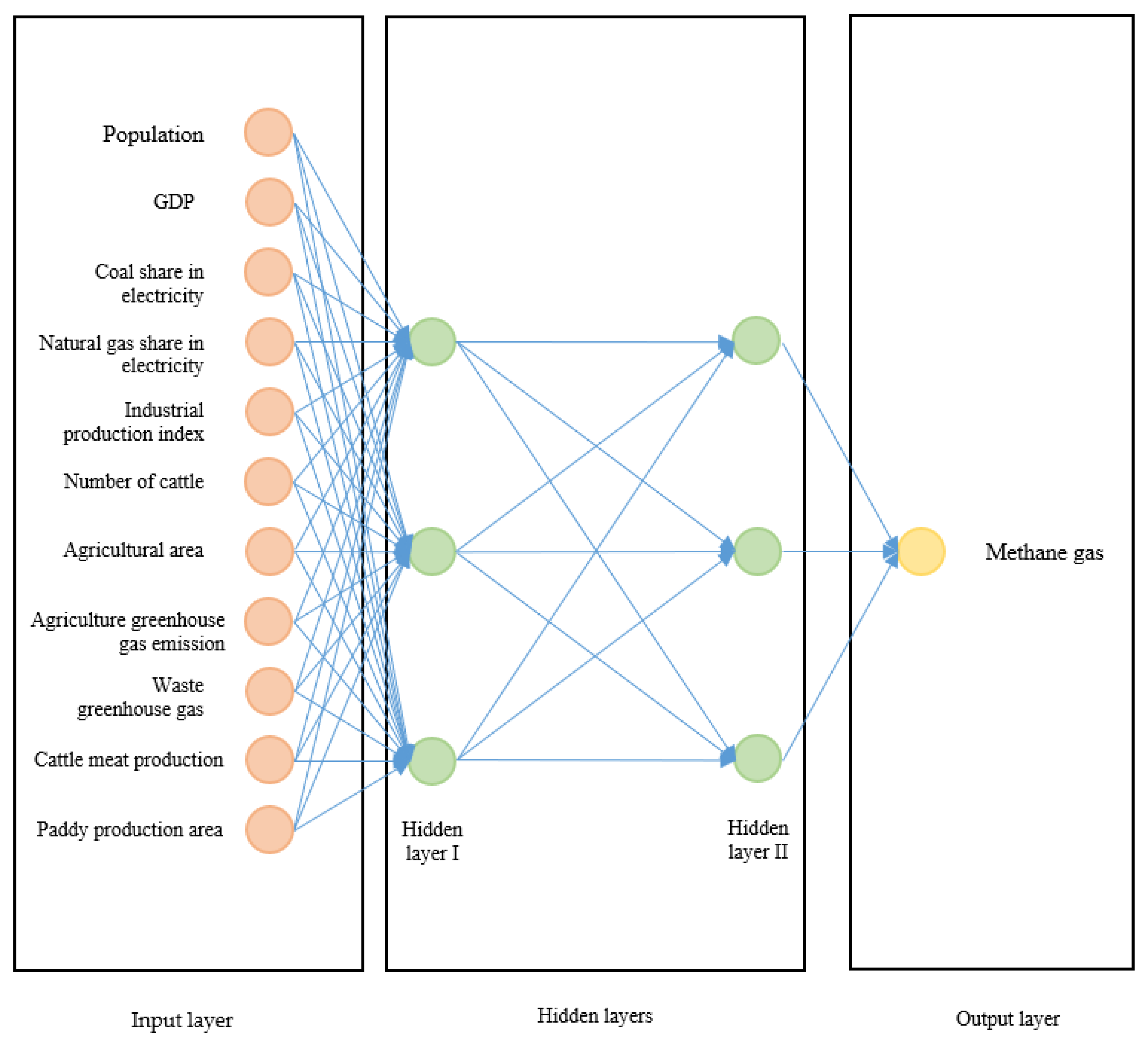
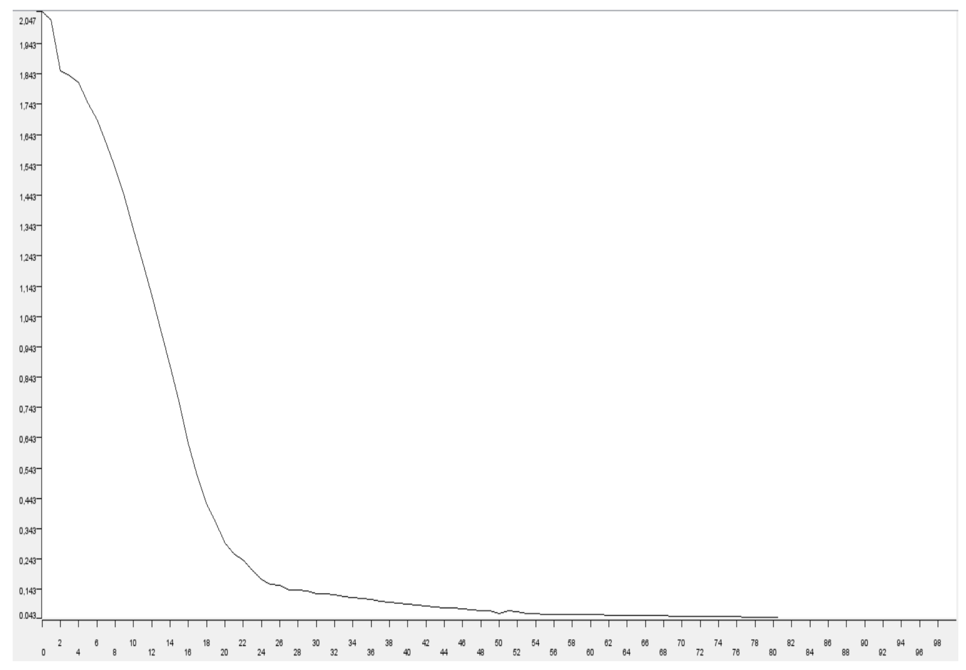
2.2.2. Artificial Neural Networks
2.2.3. Support Vector Regression
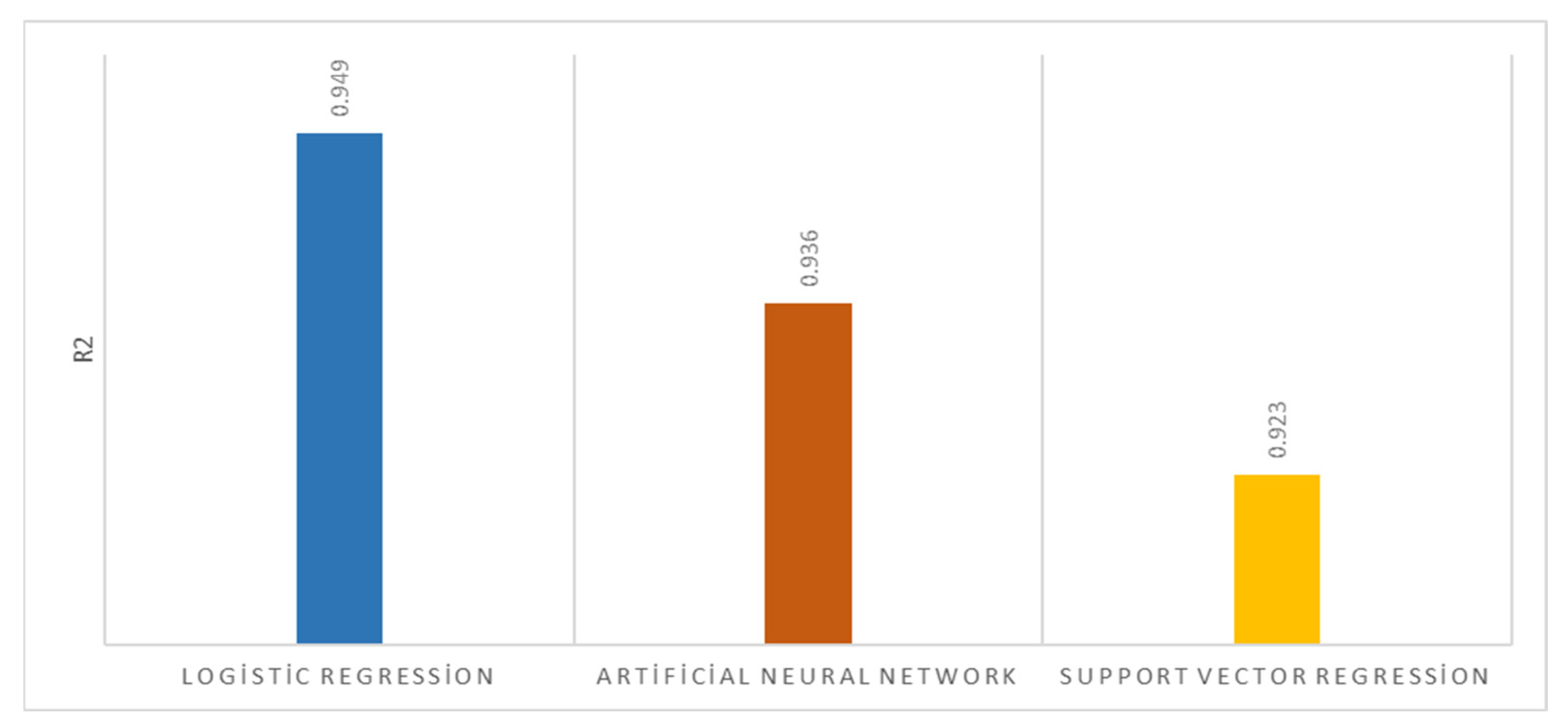
3. Results and Discussion
4. Conclusions
Author Contributions
Funding
Data Availability Statement
Conflicts of Interest
References
- Sands, P. The United Nations framework convention on climate change. Rev. Eur. Comp. Int’l Envtl. L. 1992, 1, 270. [Google Scholar] [CrossRef]
- Bodansky, D. The United Nations framework convention on climate change: A commentary. Yale J. Int’l l. 1993, 18, 451. [Google Scholar]
- Lindzen, R.S. Climate dynamics and global change. Annu. Rev. Fluid Mech. 1994, 26, 353–378. [Google Scholar] [CrossRef]
- Thuiller, W. Climate change and the ecologist. Nature 2007, 448, 550–552. [Google Scholar] [CrossRef] [PubMed]
- C. (COP27). Assessment Reports. Şarm El-Şeyh Egypt. 2022. Available online: https://cop27.eg/#/ (accessed on 10 March 2023).
- Anika, O.C.; Nnabuife, S.G.; Bello, A.; Okoroafor, R.E.; Kuang, B.; Villa, R. Prospects of Low and Zero-Carbon Renewable fuels in 1.5-Degree Net Zero Emission Actualisation by 2050: A Critical Review. Carbon Capture Sci. Technol. 2022, 5, 100072. [Google Scholar] [CrossRef]
- Pierrehumbert, R. There is no Plan B for dealing with the climate crisis. Bull. At. Sci. 2019, 75, 215–221. [Google Scholar] [CrossRef]
- Oertel, C.; Matschullat, J.; Zurba, K.; Zimmermann, F.; Erasmi, S. Greenhouse gas emissions from soils—A review. Geochemistry 2016, 76, 327–352. [Google Scholar] [CrossRef]
- Garip, E.; Oktay, A.B. Forecasting CO2 Emission with Machine Learning Methods. In Proceedings of the 2018 International Conference on Artificial Intelligence and Data Processing (IDAP), Malatya, Turkey, 28–30 September 2018. [Google Scholar]
- Baareh, A.K. Solving the carbon dioxide emission estimation problem: An artificial neural network model. J. Softw. Eng. Appl. 2013, 6, 338–342. [Google Scholar] [CrossRef]
- Kalra, S.; Lamba, R.; Sharma, M. Machine learning based analysis for relation between global temperature and concentrations of greenhouse gases. J. Inf. Optim. Sci. 2020, 41, 73–84. [Google Scholar] [CrossRef]
- Hamrani, A.; Akbarzadeh, A.; Madramootoo, C.A. Machine learning for predicting greenhouse gas emissions from agricultural soils. Sci. Total Environ. 2020, 741, 140338. [Google Scholar] [CrossRef] [PubMed]
- Saha, D.; Basso, B.; Robertson, G.P. Machine learning improves predictions of agricultural nitrous oxide (N2O) emissions from intensively managed cropping systems. Environ. Res. Lett. 2020, 16, 024004. [Google Scholar] [CrossRef]
- Gholami, H.; Mohamadifar, A.; Sorooshian, A.; Jansen, J.D. Machine-learning algorithms for predicting land susceptibility to dust emissions: The case of the Jazmurian Basin, Iran. Atmos. Pollut. Res. 2020, 11, 1303–1315. [Google Scholar] [CrossRef]
- Şişeci Çeşmeli, M.; Pençe, I. Forecasting of Greenhouse Gas Emissions in Turkey using Machine Learning Methods. Acad. Platf. J. Eng. Sci. 2020, 8, 332–348. [Google Scholar]
- Aydin, S.G.; Aydoğdu, G. CO2 Emissions in Turkey and EU Countries Using Machine Learning Algorithms. Eur. J. Sci. Technol. 2022, 37, 42–46. [Google Scholar]
- Abbasi, N.A.; Hamrani, A.; Madramootoo, C.A.; Zhang, T.; Tan, C.S.; Goyal, M.K. Modelling carbon dioxide emissions under a maize-soy rotation using machine learning. Biosyst. Eng. 2021, 212, 1–18. [Google Scholar] [CrossRef]
- Kerimov, B.; Chernyshev, R. Review of machine learning methods in the estimation of greenhouse gas emissions. In Proceedings of the International Conference of Young Scientists Modern Problems of Earth Sciences, Tbilisi, Georgia, 21–22 November 2022. [Google Scholar]
- Saleh, C.; Dzakiyullah, N.R.; Nugroho, J.B. Carbon dioxide emission prediction using support vector machine. IOP Conf. Ser. Mater. Sci. Eng. 2016, 114, 012148. [Google Scholar] [CrossRef]
- Jiang, Z.; Yang, S.; Smith, P.; Pang, Q. Ensemble machine learning for modeling greenhouse gas emissions at different time scales from irrigated paddy fields. Field Crop. Res. 2023, 292, 108821. [Google Scholar] [CrossRef]
- Ghaderzadeh, M.; Asadi, F.; Hosseini, A.; Bashash, D.; Abolghasemi, H.; Roshanpour, A. Machine Learning in Detection and Classification of Leukemia Using Smear Blood Images: A Systematic Review. Sci. Program. 2021, 2021, 9933481. [Google Scholar] [CrossRef]
- El Naqa, I.; Murphy, M.J. What is Machine Learning? Springer: Berlin/Heidelberg, Germany, 2015. [Google Scholar]
- Haldorai, A.; Ramu, A.; Suriya, M. Organization internet of things (IoTs): Supervised, unsupervised, and reinforcement learning. In Business Intelligence for Enterprise Internet of Things; Springer: Berlin/Heidelberg, Germany, 2020; pp. 27–53. [Google Scholar]
- Sperandei, S. Understanding logistic regression analysis. Biochem. Med. 2014, 24, 12–18. [Google Scholar] [CrossRef]
- Bayaga, A. Multinomial Logistic Regression: Usage and Application in Risk Analysis. J. Appl. Quant. Methods 2010, 5, 288–298. [Google Scholar]
- Hailpern, S.M.; Visintainer, P.F. Odds Ratios and Logistic Regression: Further Examples of their use and Interpretation. Stata J. Promot. Commun. Stat. Stata 2003, 3, 213–225. [Google Scholar] [CrossRef]
- Travassos, X.L.; Avila, S.L.; Ida, N. Artificial Neural Networks and Machine Learning techniques applied to Ground Penetrating Radar: A review. Appl. Comput. Inform. 2018, 17, 296–308. [Google Scholar] [CrossRef]
- Dongare, A.D.; Kharde, R.R.; Kachare, A.D. Introduction to artificial neural network. Int. J. Eng. Innov. Technol. 2012, 2, 189–194. [Google Scholar]
- Mansoor, M.; Grimaccia, F.; Leva, S.; Mussetta, M. Comparison of echo state network and feed-forward neural networks in electrical load forecasting for demand response programs. Math. Comput. Simul. 2020, 184, 282–293. [Google Scholar] [CrossRef]
- Vapnik, V. The Nature of Statistical Learning Theory; Springer Science & Business Media: Berlin/Heidelberg, Germany, 1999. [Google Scholar]
- Vapnik, V.N. An overview of statistical learning theory. IEEE Trans. Neural Netw. 1999, 10, 988–999. [Google Scholar] [CrossRef]
- Hao, P.-Y.; Kung, C.-F.; Chang, C.-Y.; Ou, J.-B. Predicting stock price trends based on financial news articles and using a novel twin support vector machine with fuzzy hyperplane. Appl. Soft Comput. 2020, 98, 106806. [Google Scholar] [CrossRef]
- Gu, B.; Sheng, V.S.; Tay, K.Y.; Romano, W.; Li, S. Cross Validation Through Two-Dimensional Solution Surface for Cost-Sensitive SVM. IEEE Trans. Pattern Anal. Mach. Intell. 2016, 39, 1103–1121. [Google Scholar] [CrossRef]
- Migilinskas, D.; Ustinovichius, L. Normalization in the selection of construction alternatives. Int. J. Manag. Decis. Mak. 2007, 8, 623–639. [Google Scholar]
- Saranya, C.; Manikandan, G. A study on normalization techniques for privacy preserving data mining. Int. J. Eng. Technol. 2013, 5, 2701–2704. [Google Scholar]
- Stone, M. Cross-validation: A review. Stat. A J. Theor. Appl. Stat. 1978, 9, 127–139. [Google Scholar]
- Picard, R.P.; Cook, R.D. Cross-validation of regression models. J. Am. Stat. Assoc. 1984, 79, 575–583. [Google Scholar] [CrossRef]
- Ozer, D.J. Correlation and the coefficient of determination. Psychol. Bull. 1985, 97, 307–315. [Google Scholar] [CrossRef]
- Di Bucchianico, A. Coefficient of determination (R2). In Encyclopedia of Statistics in Quality and Reliability; Wiley Online Library: Hoboken, NJ, USA, 2008. [Google Scholar]
- Willmott, C.J.; Matsuura, K. Advantages of the mean absolute error (MAE) over the root mean square error (RMSE) in assessing average model performance. Clim. Res. 2005, 30, 79–82. [Google Scholar] [CrossRef]
- Chai, T.; Draxler, R.R. Root mean square error (RMSE) or mean absolute error (MAE)?—Arguments against avoiding RMSE in the literature. Geosci. Model Dev. 2014, 7, 1247–1250. [Google Scholar] [CrossRef]
- Wallach, D.; Goffinet, B. Mean squared error of prediction as a criterion for evaluating and comparing system models. Ecol. Model. 1989, 44, 299–306. [Google Scholar] [CrossRef]
- Tuchler, M.; Singer, A.; Koetter, R. Minimum mean squared error equalization using a priori information. IEEE Trans. Signal Process. 2002, 50, 673–683. [Google Scholar] [CrossRef]


| Author Details | Topic | Input/Output Variables | Machine Learning Technique | Conclusion |
|---|---|---|---|---|
| (Oertel et al., 2016) [8] | Greenhouse gas emission and parameters affecting the emission process | Input: Literature review was conducted. Output: According to the result of the literature review, it was revealed that 300 mg CO2 leads to a global annual net soil emission of ≥350 Pg CO2e. | The study is based on a literature review. | The author discussed the parameters related to soil emission (by reviewing the literature). |
| (Garip and Oktay, 2018) [9] | Estimation of carbon dioxide emissions | Input: Oil, natural gas, coal, hydropower, renewable energy. Output: In the CO2 forecasts between 2004 and 2014, it was observed that the forecasts were successful in the first years and the success in the forecasts decreased in the last two years. |
| It was observed that support vector machines gave better results than the random forest regression method. |
| (Baareh, 2013) [10] | Estimation of carbon dioxide emissions | Inputs: Oil, natural gas, coal, primary energy consumption. Output: Data from 1982 to 2000 were used and found to have high predictive ability. |
| The artificial neural network model was found to have high forecasting ability. |
| (Kalra et al., 2020) [11] | Measurement of the relationship between global temperature and greenhouse gas concentration | Input: Carbon dioxide, nitrous oxide, methane. Output: In the 65 years of global temperature data between 1850 and 2016, they found that CO2 increased to the maximum in the global temperature increase. |
| It was observed that the best performance was obtained from the artificial neural network method. |
| (Hamrani et al., 2020) [12] | Estimation of greenhouse gas emissions | Input: Carbon dioxide and nitrous oxide. Output: In the 5-year period from 2012 to 2017, the LSTM model was found to give the most accurate performance. |
| It was observed that the best performance was obtained from the LSTM model. |
| (Saha et al., 2021) [13] | Estimation of agricultural nitrous oxide emissions | Input: Nitrous oxide. Output: 1576 daily observations over a 6-year period from 2002 to 2014 were used. The random forest regression model was able to predict nitrous oxide data in two different fields. |
| It was found that the random forest regression model can improve nitrous oxide flux predictions with limited data. |
| (Gholami et al., 2020) [14] | Using machine learning for dust emission sensitization in Iran | Inputs: Land use, lithology, digital elevation, vegetation cover, wind speed, rainfall, bulk density, organic matter, electrical conductivity, texture, soil texture, exchangeable sodium content and calcium carbonate content, soil property. Output: The analysis of these 14 inputs revealed that there was no multicollinearity between the inputs. CForest was found to make the best prediction. |
| It was observed that CForest algorithm made the best prediction. |
| (Şişeci Çeşmeli and Pençe, 2020) [15] | Greenhouse gas estimation for Turkey using machine learning algorithms | Input: Greenhouse gases data set for 1967–2017 (as time series). Output: Tested with time series and 10-fold cross-validation, the LTSM model was the most successful and estimated 15.67 billion tons of greenhouse gas emissions prospectively. |
| It was observed that LSTM made the best estimation. |
| (Gümüştekin Aydın and Aydoğdu, 2022) [16] | Carbon dioxide emission estimation of Turkey and EU countries using machine learning algorithms | Input: Consumption of “total population, solid fossil fuel, natural gas, oil, solar energy, biogas, primary solid biofuel, renewable municipal waste, geothermal energy and hydropower” from 2000 to 2019. Output: It was observed that the amount of CO2 decreased in EU countries and the amount of CO2 increased exponentially in Turkey. |
| It was seen that the support vector machines method made the best prediction. |
| (Abbasi et al., 2021) [17] | Estimation of carbon dioxide emissions through machine learning algorithms | Inputs: Soil moisture, temperature, organic matter, total carbon, nitrogen, air temperature, solar radiation, rainfall, pan evaporation. Output: Soil temperature, organic matter, carbon, nitrogen, air temperature, radiation and pan evaporation were found to be highly correlated parameters. |
| It was observed that the random forest regression method made the best prediction. |
| (Kerimov and Chernyshev, 2022) [18] | Estimation of greenhouse gas emissions through machine learning algorithms | A research study was conducted to define the model structure. |
| The study compared the advantages and disadvantages of the techniques. |
| (Saleh et al., 2016) [19] | Estimation of carbon dioxide emissions using support vector machines | Input: Electric power and coal Output: The support vector machines method was used by trial and error. The results showed that the RMSE value was 0.004, but the aim was to obtain a value lower than this. |
| In the study, it was concluded that the RMSE value was higher than expected. It was predicted that a lower value would lead to a higher prediction and a higher prediction would provide information about CO2 emission. |
| (Jiang et al., 2023) [20] | Estimation of greenhouse gas emissions in paddy fields in China through machine learning algorithms | Input: 3-year data set from 2009 to 2011. Output: The stacking model improved R2 and reduced RMSE. |
| It was found that the stacking model was the best prediction method, and the linear regression model was the worst prediction method. |
| Output Variable | Input Variables | |
|---|---|---|
| Methane Gas Emissions (tons) | Agricultural Activities | Number of Cattle (pcs) |
| Red Meat Production (tons) | ||
| Agricultural Area (hectare) | ||
| Agricultural Greenhouse Gas Emissions (tons) | ||
| Paddy Production (hectare) | ||
| Energy | Share of Coal in Total Energy Production (%) | |
| Share of Natural Gas in Total Energy Production (%) | ||
| Industrial Production Index (2003 = 100) | ||
| Waste | Waste Greenhouse Gas Emission (tons) | |
| General | Population (Number of People) | |
| GDP ($) | ||
| Average | Maximum | Minimum | SD | |
|---|---|---|---|---|
| Methane gas | 48,868,492 | 63,988,980 | 40,945,943 | 7,131,161 |
| Population | 68,251,387 | 83,614,362 | 53,921,758 | 9,039,080 |
| GDP | 506,221,633,744 | 957,783,020,853 | 130,690,172,297 | 301,529,901,430 |
| Coal share in electricity | 30.72 | 37.20 | 22.80 | 4.05 |
| Natural gas share in electricity | 33.88 | 49.70 | 14.60 | 12.25 |
| Industrial production index | 70.59 | 144.69 | 33.13 | 34.52 |
| Number of cattle | 12,580,168 | 18,157,971 | 9,901,458 | 2,275,392 |
| Agricultural area | 39,389,935 | 42,033,000 | 37,716,000 | 1,160,451 |
| Agriculture greenhouse gas emission | 48,621,599 | 73,155,372 | 37,607,794 | 9,063,809 |
| Waste greenhouse gas emission | 15,132,177 | 17,786,989 | 11,080,826 | 2,168,268 |
| Cattle meat production | 614,882 | 1,341,445 | 303,120 | 313,293 |
| Paddy production area | 82,125 | 126,419 | 40,400 | 29,149 |
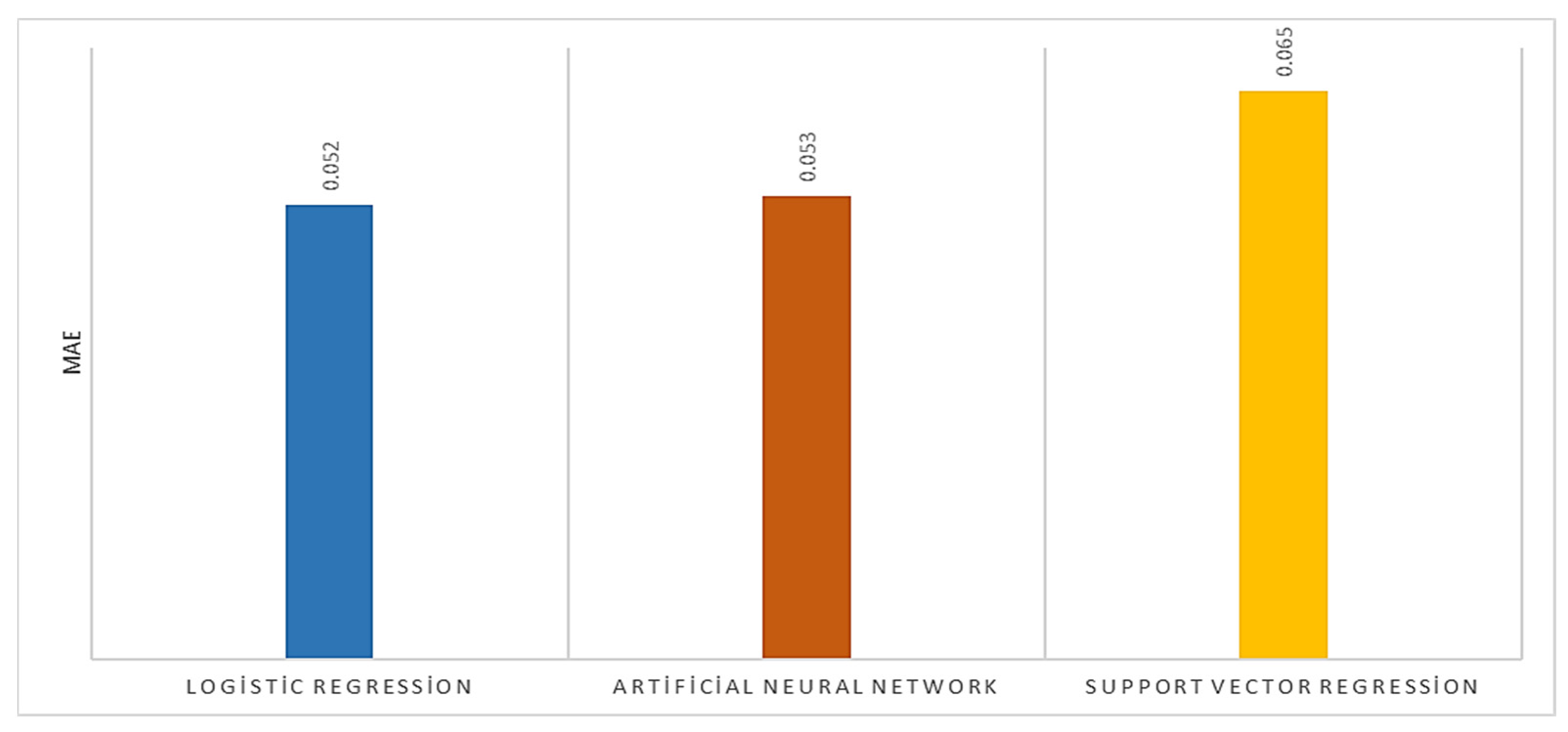
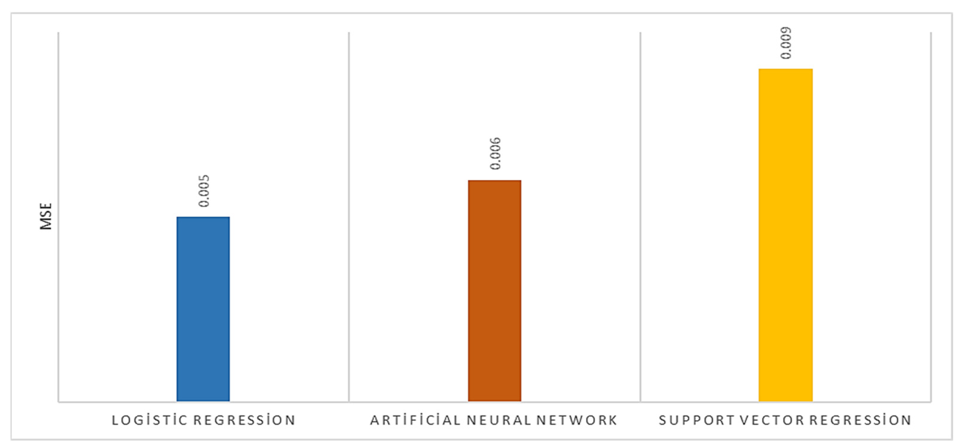
| Logistic Regression | Artificial Neural Network | Support Vector Regression | |
|---|---|---|---|
| R2 | 0.949 | 0.936 | 0.923 |
| MAE | 0.052 | 0.053 | 0.065 |
| MSE | 0.005 | 0.006 | 0.009 |
Disclaimer/Publisher’s Note: The statements, opinions and data contained in all publications are solely those of the individual author(s) and contributor(s) and not of MDPI and/or the editor(s). MDPI and/or the editor(s) disclaim responsibility for any injury to people or property resulting from any ideas, methods, instructions or products referred to in the content. |
© 2023 by the authors. Licensee MDPI, Basel, Switzerland. This article is an open access article distributed under the terms and conditions of the Creative Commons Attribution (CC BY) license (https://creativecommons.org/licenses/by/4.0/).
Share and Cite
Ünal Uyar, G.F.; Terzioğlu, M.; Kayakuş, M.; Tutcu, B.; Çoşgun, A.; Tonguç, G.; Kaplan Yildirim, R. Estimation of Methane Gas Production in Turkey Using Machine Learning Methods. Appl. Sci. 2023, 13, 8442. https://doi.org/10.3390/app13148442
Ünal Uyar GF, Terzioğlu M, Kayakuş M, Tutcu B, Çoşgun A, Tonguç G, Kaplan Yildirim R. Estimation of Methane Gas Production in Turkey Using Machine Learning Methods. Applied Sciences. 2023; 13(14):8442. https://doi.org/10.3390/app13148442
Chicago/Turabian StyleÜnal Uyar, Güler Ferhan, Mustafa Terzioğlu, Mehmet Kayakuş, Burçin Tutcu, Ahmet Çoşgun, Güray Tonguç, and Rüya Kaplan Yildirim. 2023. "Estimation of Methane Gas Production in Turkey Using Machine Learning Methods" Applied Sciences 13, no. 14: 8442. https://doi.org/10.3390/app13148442
APA StyleÜnal Uyar, G. F., Terzioğlu, M., Kayakuş, M., Tutcu, B., Çoşgun, A., Tonguç, G., & Kaplan Yildirim, R. (2023). Estimation of Methane Gas Production in Turkey Using Machine Learning Methods. Applied Sciences, 13(14), 8442. https://doi.org/10.3390/app13148442