A Comparative Regression Analysis between Principal Component and Partial Least Squares Methods for Flight Load Calculation

Featured Application

This study investigates and compares various multivariate regression methods, including principal component regression (PCR) and partial least squares regression (PLSR), for flight load analysis and demonstrates their high learning efficiency and strong generalization capabilities, making them highly suitable for this purpose.

Abstract

This study investigates and compares various multivariate regression methods, including principal component regression (PCR) and partial least squares regression (PLSR), for flight load analysis and demonstrates their high learning efficiency and strong generalization capabilities, making them highly suitable for this purpose. The flight load data of a civil aircraft use altitude, Mach number and load factors as input parameters, which are used as sample data to establish regression models for predicting wing loads under different flight conditions. The accuracy of all regressions are confirmed through evaluation, with PLSR being the most efficient. In the comparison of computational times, it was found that the computational efficiency of regression methods was significantly superior to traditional panel methods. The flight load calculation shows that PCR and PLSR can significantly improve analysis efficiency and provide new insights into efficient flight load analysis.

1. Introduction

The flight load refers to the load borne by the aircraft during the entire flight process from takeoff to landing. The main purpose of conducting flight load analysis is to identify the most severe load conditions for different aircraft components in different flight states [1]. The results of flight load analysis show the magnitude and distribution of the load on the aircraft structure, which is an important basis for aircraft structural strength design. In recent years, with the extensive use of composite materials in civil aircraft, it has brought benefits of weight reduction to the aircraft, but also posed new requirements for strength and structural design [2]. Therefore, flight load calculation and analysis is an important part of civil aircraft design.

During flight, an aircraft is subjected to a variety of external forces, such as aerodynamic, gravitational, and inertial forces. These forces can vary significantly depending on factors such as airspeed, altitude, maneuvering, and atmospheric conditions. Flight load analysis aims to determine the magnitudes and distributions of these forces on different parts of the aircraft, including the fuselage, wings, tails, and landing gear.

Traditional flight load design has been well developed and has achieved many results, including engineering design examples and scientific research papers. In engineering applications, different flight parameters, including airspeed, altitude, and maneuvering capabilities, are selected based on the aircraft model to construct flight envelopes. Then, CFD calculations [3,4] or wind tunnel calculations [5] are performed on the component loads within the flight envelope to establish a component load database. The load distribution of the components and the entire aircraft is determined based on static aeroelastic analysis, and the severe load conditions of the components are selected as important basis for aircraft structural strength design.

Due to the large number of flight load calculations that can reach the millions, the computational resources required for flight load analysis are enormous, and the cycle of analysis is very long. In order to solve this problem, various methods have been developed, such as low-order panel methods and high-order panel methods. However, each method has its own obvious drawbacks. The low-order panel method [6] provides two-dimensional results with low accuracy, and it is only suitable for the early design stage of the aircraft. On the other hand, although the high-order panel method [7,8] has guaranteed accuracy and significantly reduces the computation time compared to CFD-CSD coupled calculations, it still requires significant computational resources for millions of aircraft load calculations. In this case, surrogate models based on numerical regression and neural networks have made a lot of progress and achievements in reducing the flight load calculation process. Li HQ et al. demonstrate the potential of deep learning-based regression models in improving efficiency and accuracy of aircraft structural design for flight loads calculations [9]. Sykes BS et al. introduce a novel alternative reduced order model that improves the accuracy of predicting loads induced by aircraft lateral oscillation by 150% compared to a fixed fuel mass model [10]. Lee D et al. utilize cluster Kriging and machine learning techniques to accurately represent the complex physical relationships of aeroelastic responses, resulting in significant vibration reduction during high-speed flights for composite rotor blades [11]. These studies demonstrate that flight load surrogate model techniques simplify the cumbersome traditional flight load calculation methods and have significant potential for application [12].

By contrast, the aerodynamic load analysis based on feature value analysis and partial least squares regression remains a blank space at present. Compared with models based on neural networks, the principal component regression model’s main advantage is its ability to effectively eliminate the multi-collinearity that influences the relationships between variables, to utilize redundant information among the initial variables, and to maintain interpretable and operable features, effectively handling multidimensional data in large-scale datasets. Partial least squares regression (PLSR) can be regarded as an improved version of PCR, as it ensures that the regression model takes into account the essential correlations between the X and Y datasets through cross-projection methods, achieving more accurate prediction results when using a small number of principal components compared to PCR.

Because of numerous benefits, PCR and PLSR are widely applied in various fields. Kim, J., et al. compared the accuracy of principal component regression (PCR) and partial least squares regression (PLSR) in predicting neurochemical concentrations from fast-scan cyclic voltammetry (FSCV) measurements and found that PLSR showed higher accuracy and selectivity than PCR, making it a more reliable tool for FSCV data analysis [13]. Li, J.T., et al. [14] compared the performance of partial least squares regression (PLSR) and improved principal component regression (PCR) in an ultraviolet spectral analysis of water quality detection. The results show that while PLSR is generally the predominant technology, the improved PCR method outperforms PLSR for data near the detection limit. Both methods rely on principal component analysis (PCA) to reduce the dimensionality of the spectral data and linear regression analysis to obtain the coefficients and relationships of the principal components. Ergon, R., et al. [15] explore the use of latent variables modeling and Kalman filtering theory to optimize PLSR and PCR predictors, based on prior X noise covariance estimates. The result is a new PLSR optimization method, while the PCR optimization is identical to a previously known method. The study includes a simulation example and two real-world data examples and is limited to cases with only one response variable. Engelen, S., et al. [16] compare robust and classical versions of principal component regression (PCR) and partial least squares regression (PLSR) in terms of efficiency, goodness-of-fit, predictive power, and robustness, as these are the two most popular regression techniques in chemometrics that fit a linear relationship between two sets of variables, with responses typically being low-dimensional and regressors being numerous. Singh, M., et al. [17] compare the performance of principal component regression (PCR) and partial least squares regression (PLSR) in analyzing the laser-induced breakdown spectroscopy (LIBS) data of stainless steel samples with multi-elemental concentration data and propose guidelines for selecting the appropriate approach based on the analytical situation. Zhang, X.G., et al. compared the performance of PLSR and PCR models in predicting soil salinity using soil spectra data and found that PLSR was superior to PCR when using the original spectral bands, but after smoothing the data, PCR performed better [18]. Polat, E., et al. compare the efficiency, goodness-of-fit, and predictive power of robust and classical versions of principal component regression (PCR) and partial least squares regression (PLSR) methods through a simulation study [19]. In summary, PCR and PLSR have a wide range of applications in many fields due to their many advantages.

In this paper, the flight load data are used as sample data to establish principal component regression (PCR) model and partial least squares (PLSR) model for predicting wing loads under different flight conditions using altitude, Mach number, and load factor as input parameters. Evaluations confirm the high prediction accuracy of two models, with PLSR being the most accurate. The accuracy of PCR and PLSR shows that these regression models can significantly improve flight load analysis efficiency and provide new insights into efficient and comprehensive flight load analysis.

The remainder of the paper is organized as follows. The methodology is detailed in Section 2. The model for flightload calculation is shown in Section 3. The results of the PCR and PLSR for flightload calculation are presented in Section 4 and Section 5 reports the conclusions.

2. Methodology

2.1. Static Aeroelastic Response Equation

The basic equation of static aeroelastic response analysis is generally stated as follows [12]:

$$[K_{ff}-\overline{q}{Q}_{ff}]u_f+M_{ff}{\ddot{u}}_f=\overline{q}{Q}_{fx}{u}_x+P_f$$

(1)

where $K_{ff}$ is the structure stiffness, $\overline{q}$ is the dynamic pressure, $u_f$ is the displacement vector, $M_{ff}$ is the structure mass matrix, and $P_f$ is the external loads. $\overline{q}{Q}_{ff}{u}_f$ is the aerodynamic increments generated by structural elastic deformation, and $\overline{q}{Q}_{fx}{u}_x$ is the aerodynamic force generated by the deflections of aerodynamic control surface and rigid body motion. The elastic aerodynamic derivatives and trim parameters were obtained from this formula.

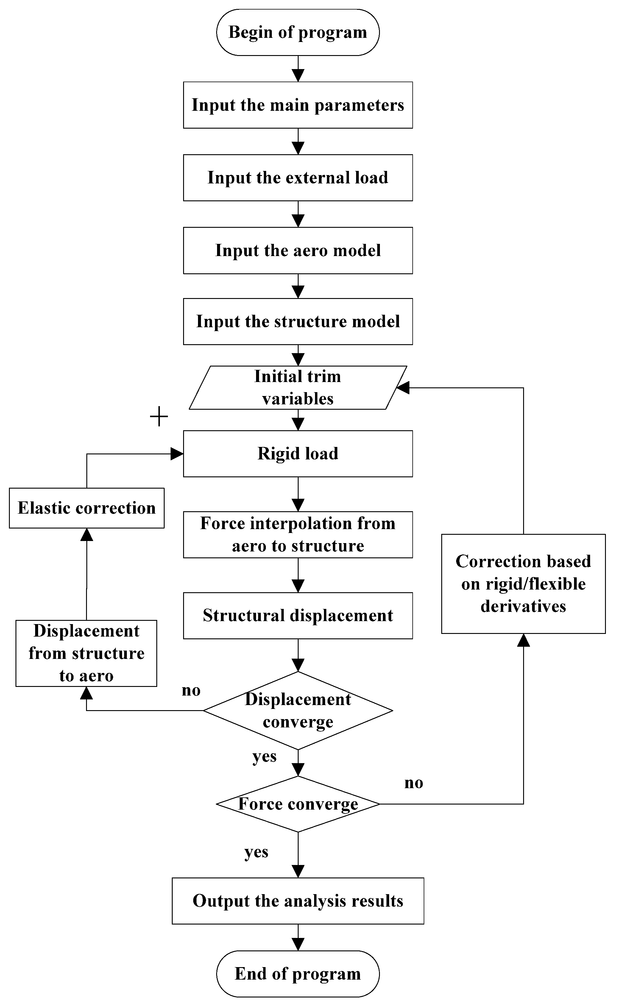
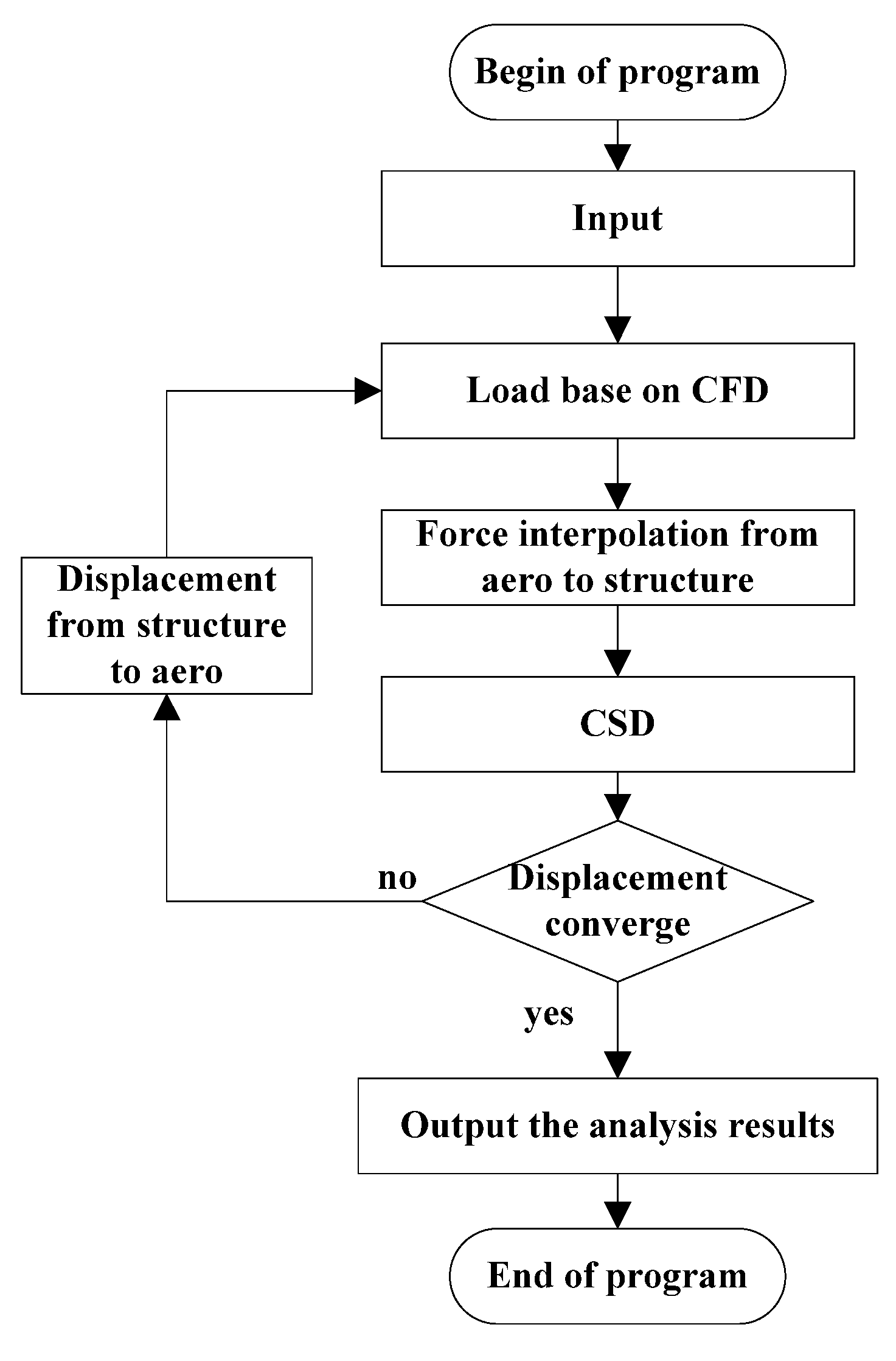
Figure 1 shows a typical iteration process for the static aeroelastic coupling computation, which includes three main steps: static aerodynamic solution, structural solution, and coupling solution. The static aerodynamic solution refers to solving the flow field equations and static aerodynamic equations to obtain the pressure and velocity distribution in the flow field. The structural solution refers to solving the structural mechanics equations to obtain the displacement and stress distribution in the structure. The coupling solution refers to using the flow field pressure and velocity distribution as boundary conditions to iteratively solve the flow field equations and structural mechanics equations to obtain the final coupled solution. The figure also shows the convergence criteria for the iterative computation and the flow control of the iteration process. The entire computation process requires multiple iterations until the convergence criteria are met.

2.2. Principal Component Analysis (PCA)

Principal component analysis (PCA) is a linear transformation technique used to reduce the dimensionality of multivariate data. It aims to capture the maximum variance within a dataset while minimizing the loss of information. By transforming the original features into linearly uncorrelated principal components, PCA provides a succinct representation of the data.

The mathematical formula for PCA is:

$$\mathrm{X}=\mathrm{US}{\mathrm{V}}^{\prime }$$

(2)

where X is the centered observation matrix, U is the matrix of scores, S is the diagonal matrix of singular values, and V is the matrix of loadings.

2.3. Principal Component Regression (PCR)

Principal component regression (PCR) is a method that combines the advantages of a principal component analysis with linear regression. It is a powerful tool for analyzing high-dimensional data when the number of observations is smaller than the number of predictor variables. PCR works by constructing a small set of principal components and then using them as predictors in a regression model.

The mathematical formula for PCA is:

$$\mathrm{Y}=\mathrm{XB}+\epsilon$$

(3)

where Y is the response variable, X is the observed predictor matrix, B is the matrix of regression coefficients, and $\epsilon$ is the vector of residual errors.

The solution of multiple linear regression is:

$$\hat{B}={({\mathrm{X}}^{\prime }\mathrm{X})}^{-1}{\mathrm{X}}^{\prime }\mathrm{Y}$$

(4)

In PCR, the collinearity that exists in the predictor variables can be eliminated by extracting a group of orthogonal predictors through the application of PCA on X and then performing regression on Y using a subset of the resulting components of X.

$$\mathrm{X}=\mathrm{US}{\mathrm{V}}^{\prime }+\epsilon$$

(5)

$$\mathrm{U}=\mathrm{XV}$$

(6)

where U is the matrix of scores, S is the diagonal matrix of singular values, and V is the matrix of loadings.

The multiple linear regression can be written as the following:

$$\mathrm{Y}=\mathrm{UB}+\epsilon$$

(7)

The solution of regression can be written as the following:

$$\hat{B}={({\mathrm{U}}^{\prime }\mathrm{U})}^{-1}{\mathrm{U}}^{\prime }\mathrm{Y}$$

(8)

2.4. Partial Least Squares Regression (PLSR)

Partial least squares regression (PLSR) is a more advanced version of PCR. It improves the predictive performance of PCR by prioritizing the predictor variables that are most strongly related to the response variable.

In PLSR, the outer relation for X, which is similar to PCA, can be written as:

$$\mathrm{X}=\mathrm{US}{\mathrm{V}}^{\prime }+\epsilon$$

(9)

$$\mathrm{U}=\mathrm{XV}$$

(10)

The Y can be written in the same way:

$$\mathrm{Y}=\mathrm{TS}{\mathrm{P}}^{\prime }+{\epsilon }^{*}$$

(11)

$$\mathrm{T}=\mathrm{YP}$$

(12)

where T is the matrix of Y scores, S is the diagonal matrix of singular values, and P is the matrix of Y loadings.

The inner relation of X and Y can be expressed by the X scores and Y scores. The model for this relation can be written as:

$${\hat{t}}_i{=\mathrm{b}}_i{\mathrm{u}}_i$$

(13)

The main difference between PLSR and PCR is that PLSR includes the linear combinations of both the predictor and response variables in the model. This results in better predictive performance and more robustness when dealing with noisy data.

2.5. Mean Absolute Error (MAE), Mean Squared Error (MSE), and Root Mean Squared Error (RMSE)

MAE, MSE and RMSE are all metrics used to evaluate the performance of a surrogate model, particularly in regression problems.

MAE (Mean Absolute Error) is a commonly used metric in statistical modeling to assess the average difference between predicted and actual values.

$$\mathrm{MAE}=\frac{1}{n}{\displaystyle \sum _{i=1}^n\left|y_i-{\hat{y}}_i\right|}$$

(14)

MSE (Mean Squared Error) is a commonly used metric in statistical modeling to assess the average squared difference between predicted and actual values.

$$\mathrm{MSE}=\frac{1}{n}{\displaystyle \sum _{i=1}^n{\left(y_i-{\hat{y}}_i\right)}^2}$$

(15)

RMSE (Root Mean Squared Error) is a widely used metric in statistical modeling to evaluate the average square root of the difference between predicted and actual values.

$$\mathrm{RMSE}=\sqrt{\mathrm{MSE}}=\sqrt{\frac{1}{n}{\displaystyle \sum _{i=1}^n{\left(y_i-{\hat{y}}_i\right)}^2}}$$

(16)

2.6. Coefficient of Determination R-Square

The coefficient of determination, also known as R-square, is a statistical measure used to assess the goodness of fit of a regression model. It evaluates the proportion of the variance in the dependent variable that can be explained by the independent variables.

R-square is typically represented as a value between 0 and 1. A value of 0 indicates that the model does not explain any of the variance in the dependent variable, while a value of 1 indicates that the model explains all of the variance [12].

R-square can be interpreted as the proportion of the variance in the dependent variable that is predictable from the independent variables in the model. However, it does not indicate the accuracy or reliability of the predictions. It is possible to have a high R-square value but still have significant errors in the predictions. Therefore, it is important to consider other evaluation metrics in conjunction with R-square when assessing the performance of a regression model.

$$\mathrm{R}-\mathrm{square}=1-\frac{{\displaystyle \sum _{i=1}^n{\left({\hat{y}}_i-y_i\right)}^2}}{{\displaystyle \sum _{i=1}^n{\left(\overline{y}-y_i\right)}^2}}=\frac{{\displaystyle \sum _{i=1}^n{\left({\hat{y}}_i-\overline{y}\right)}^2}}{{\displaystyle \sum _{i=1}^n{\left(\overline{y}-y_i\right)}^2}}$$

(17)

3. Flightload Calculation Modeling

3.1. Aircraft Model

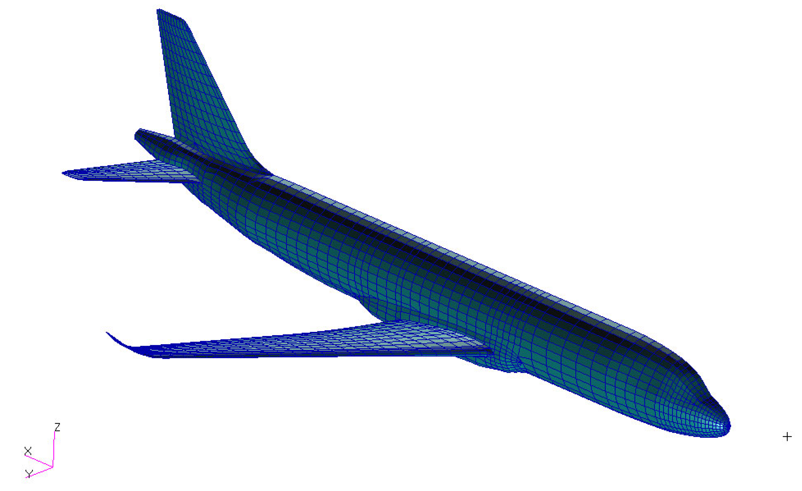
In this paper, we chose a civil aircraft to verify PCR and PLSR. The total weight of the aircraft was 77 t. The aspect ratio was 8, and the reference area was 118 m².

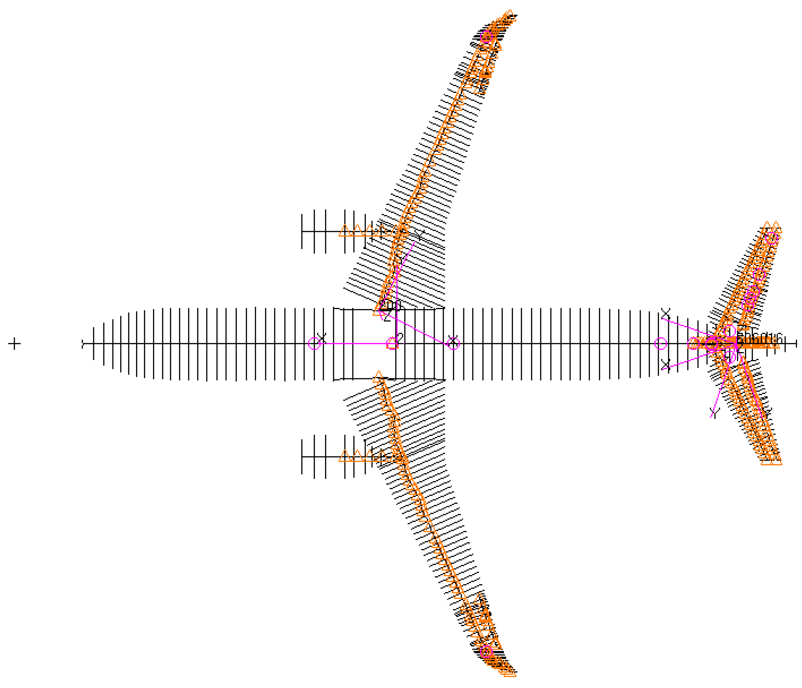
The structure model of the plane is shown in Figure 2.

The aerodynamic model of the plane is shown in Figure 3.

3.2. Data Sources and Traditional Flightload Calculation Method

In the calculation of flightload envelope, the efficient panel method was generally used instead of the computationally expensive CFD–CSD coupling method, as millions of flightload conditions needed to be calculated. Figure 4 shows the computational process of the high-order panel method used in this study. Each iteration took approximately 1 min, and each inner loop, which calculated the flightload for a fixed angle of attack, took about 2–4 min. Each outer loop, which calculated the flightload for a fixed load factor, took approximately 5–10 min. The calculation time for each flight condition was more than 5 min, so the total time for millions of flight conditions is indeed observable.

3.3. Input and Output Data

The complexity of aircraft flight loads is influenced by various input data. These loads undergo significant variations during different flight stages, such as takeoff, climb, cruise, descent, and landing. External factors like altitude, pressure, and wind speed also have a notable impact on flight loads. The output data, which represent the load status of different components of the airplane structure, vary according to specific flight load conditions. Therefore, it is crucial to carefully select flight load conditions [12].

In this study, symmetric maneuver flight is used as an example to conduct regression analysis and validation. The load of axially symmetric maneuver flight is influenced by factors such as flight altitude, Mach number, longitudinal load, pitch acceleration, angle of attack, and elevator deflection. To ensure accuracy, flight altitude, Mach number, load factor, and pitch acceleration were chosen as input parameters, while maintaining a balanced angle of attack and elevator deflection based on empirical calculations and conventions.

Table 1. Range of input parameters.

Meaning	Lower Limit	Higher Limit
Flight altitude (m)	13,359	19,429
Mach number	0.6072	0.82
Load factor	−2.5	1
Pitch acceleration	−0.2	0.2

shows the range of input parameters.

To comprehensively investigate the severe load situations of various aircraft components, typical profiles of the components need to be selected, and their corresponding shear forces, bending moments, and torque moments should be calculated to characterize their load situations. In this study, the shear forces, bending moments, and torque moments of the airplane wings were selected as output parameters.

Table 2. Output parameter.

Meaning	Unit
Shear force	N
Bending moment	N × m
Torque moment	N × m

shows the output parameter.

3.4. Training and Test Data

The data used in this study consisted of a total of 56 sets of flight load data. Using randomization, the data were divided into a training set of 46 flight load datapoints and a test set of 10 flight load datapoints.

3.5. PCR and PLSR Modeling

This article uses MATLAB for program development and regression model establishment. The main program codes for PCR and PLSR are provided in Appendix A.

4. Result and Discussion

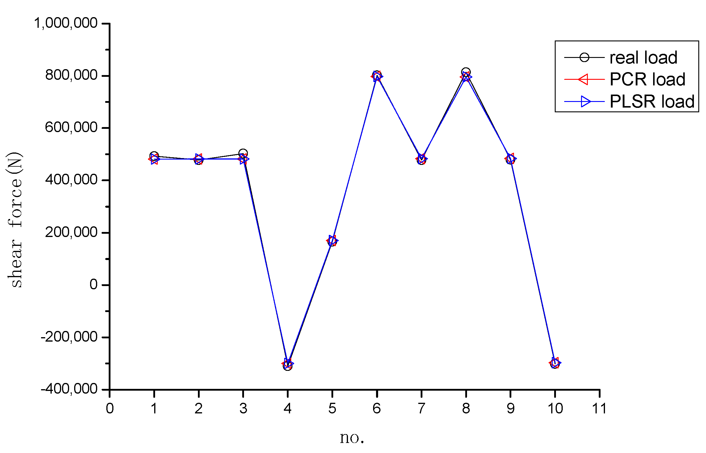
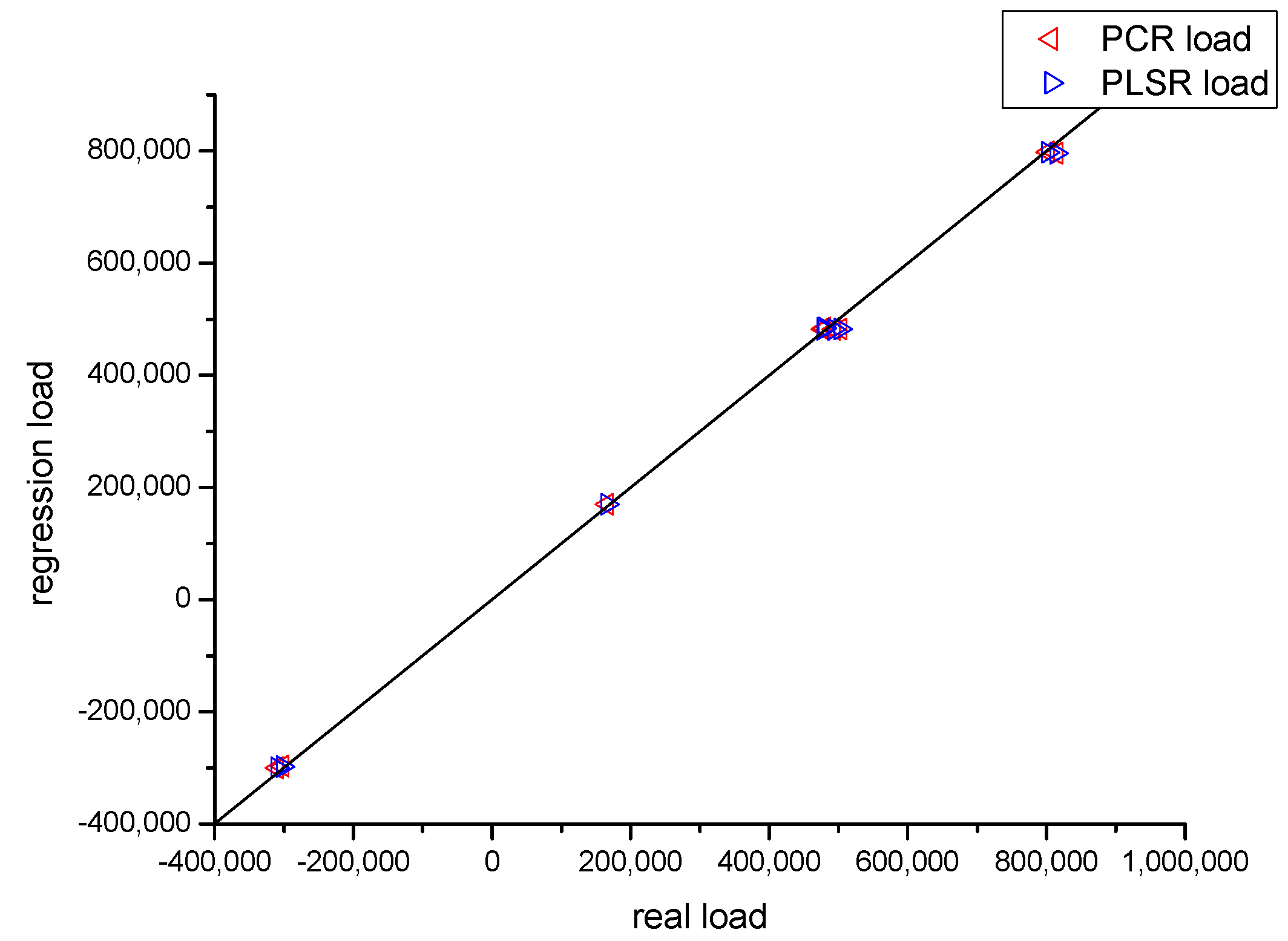
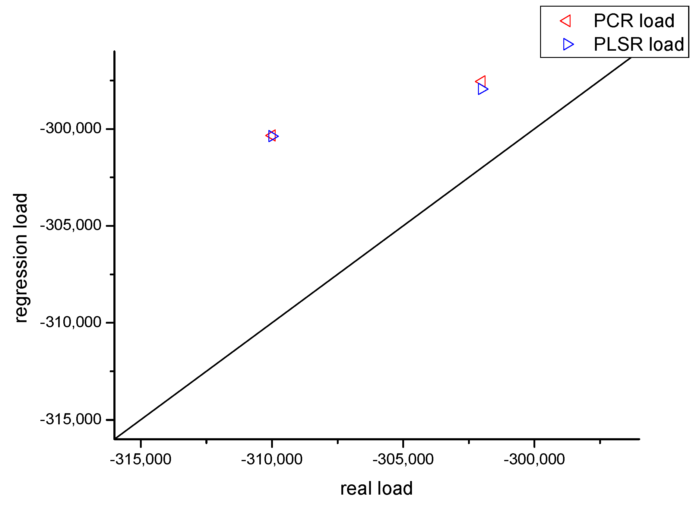
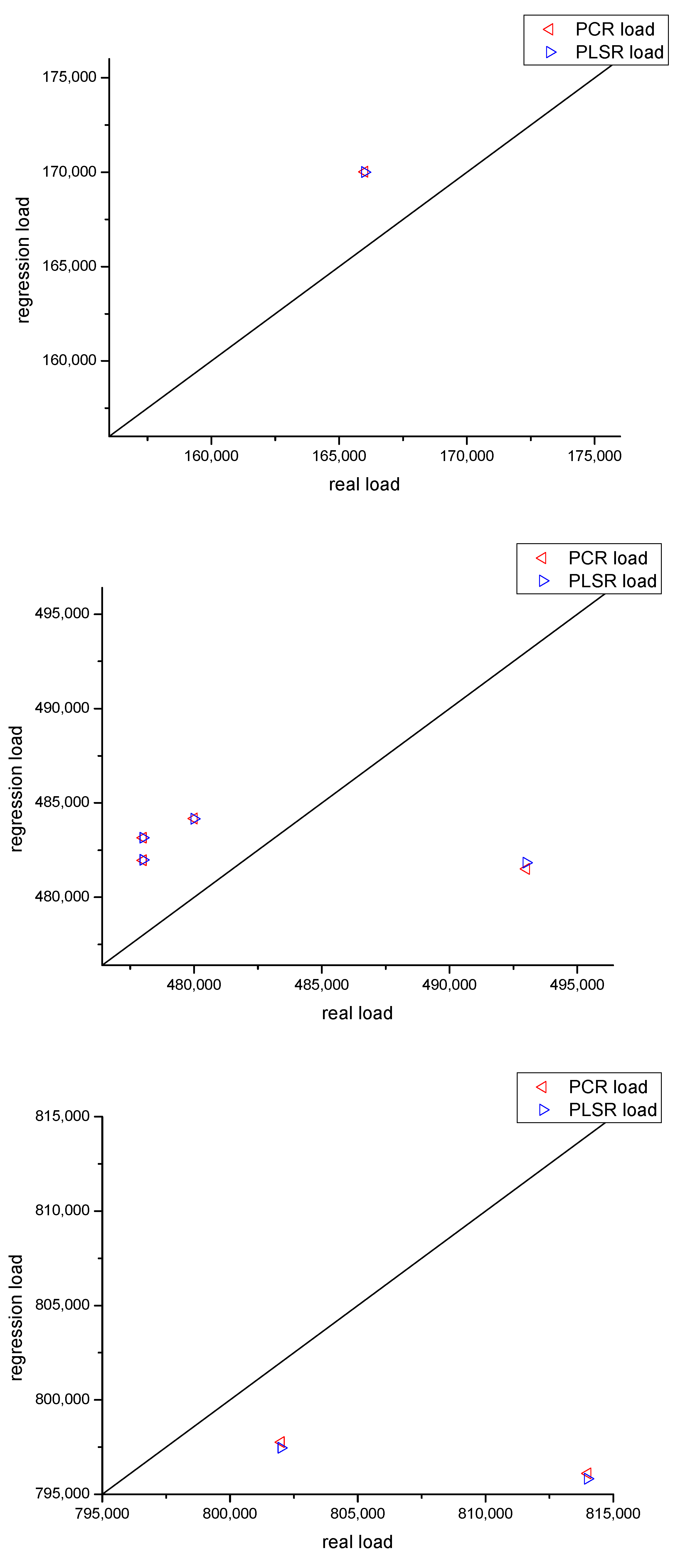
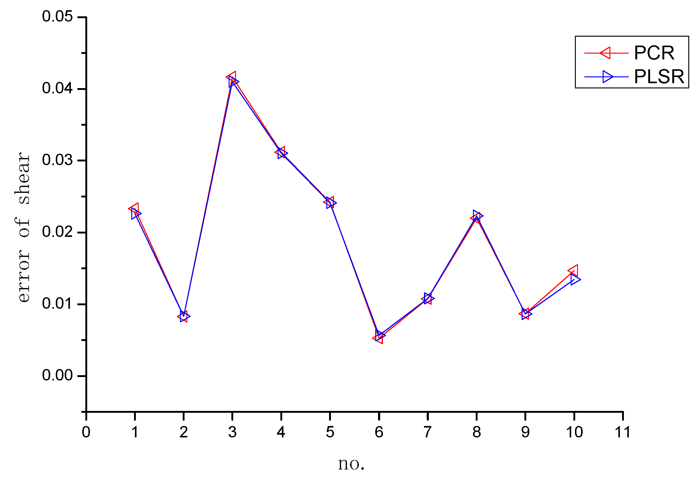
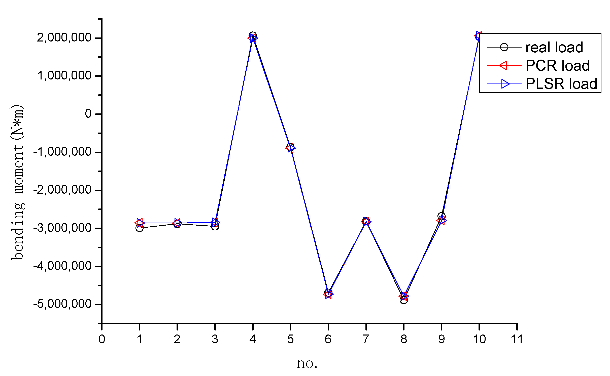
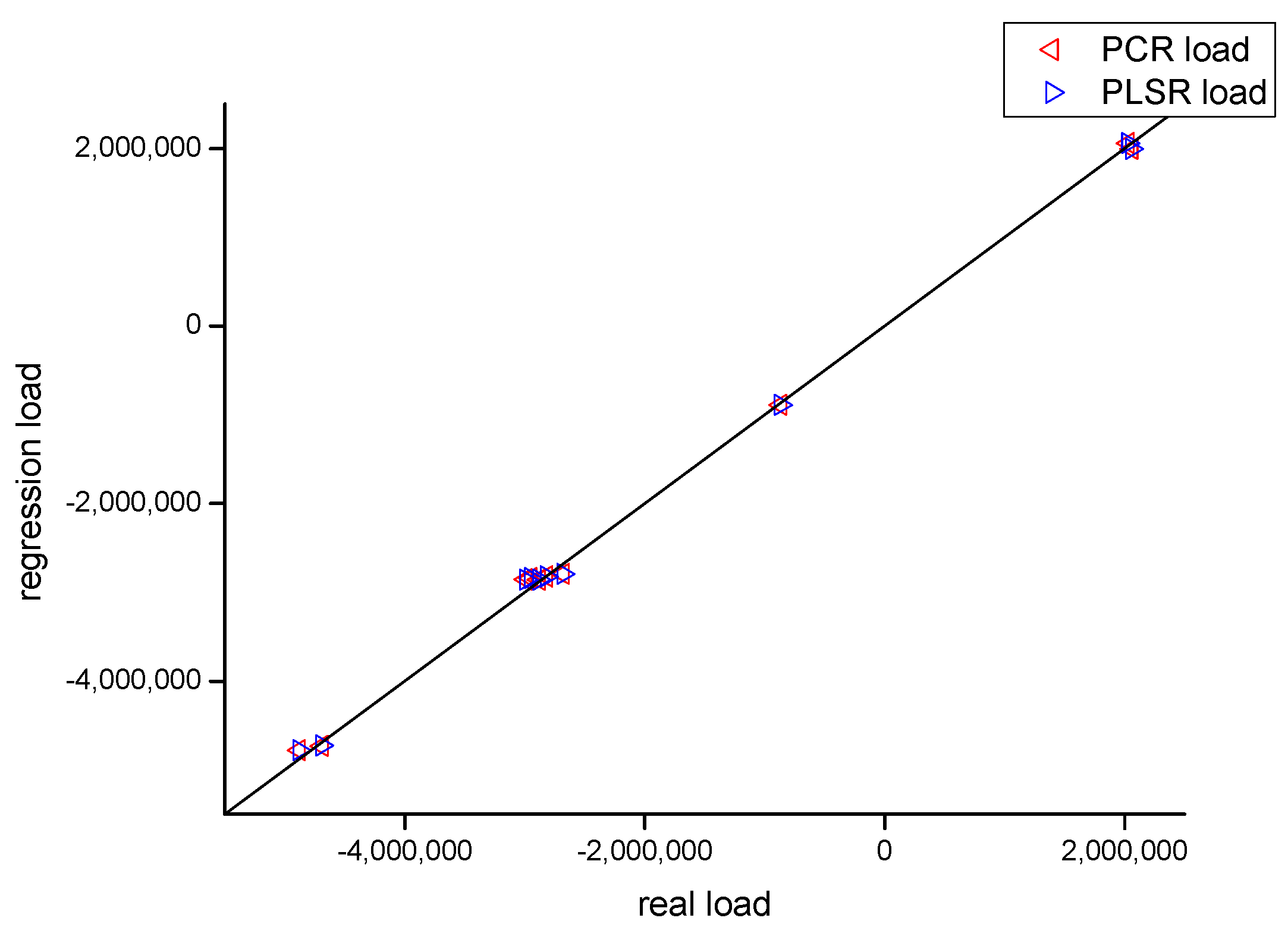
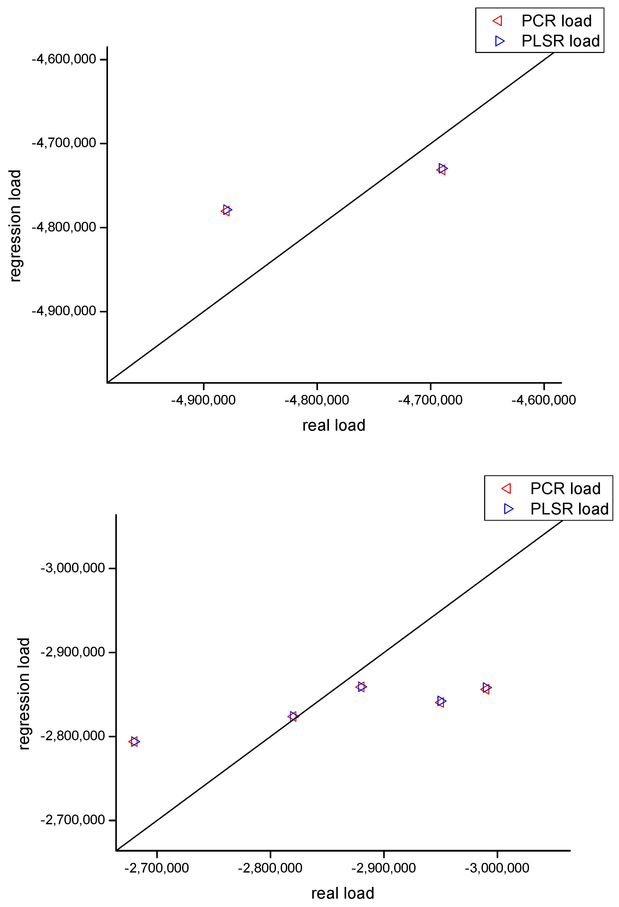
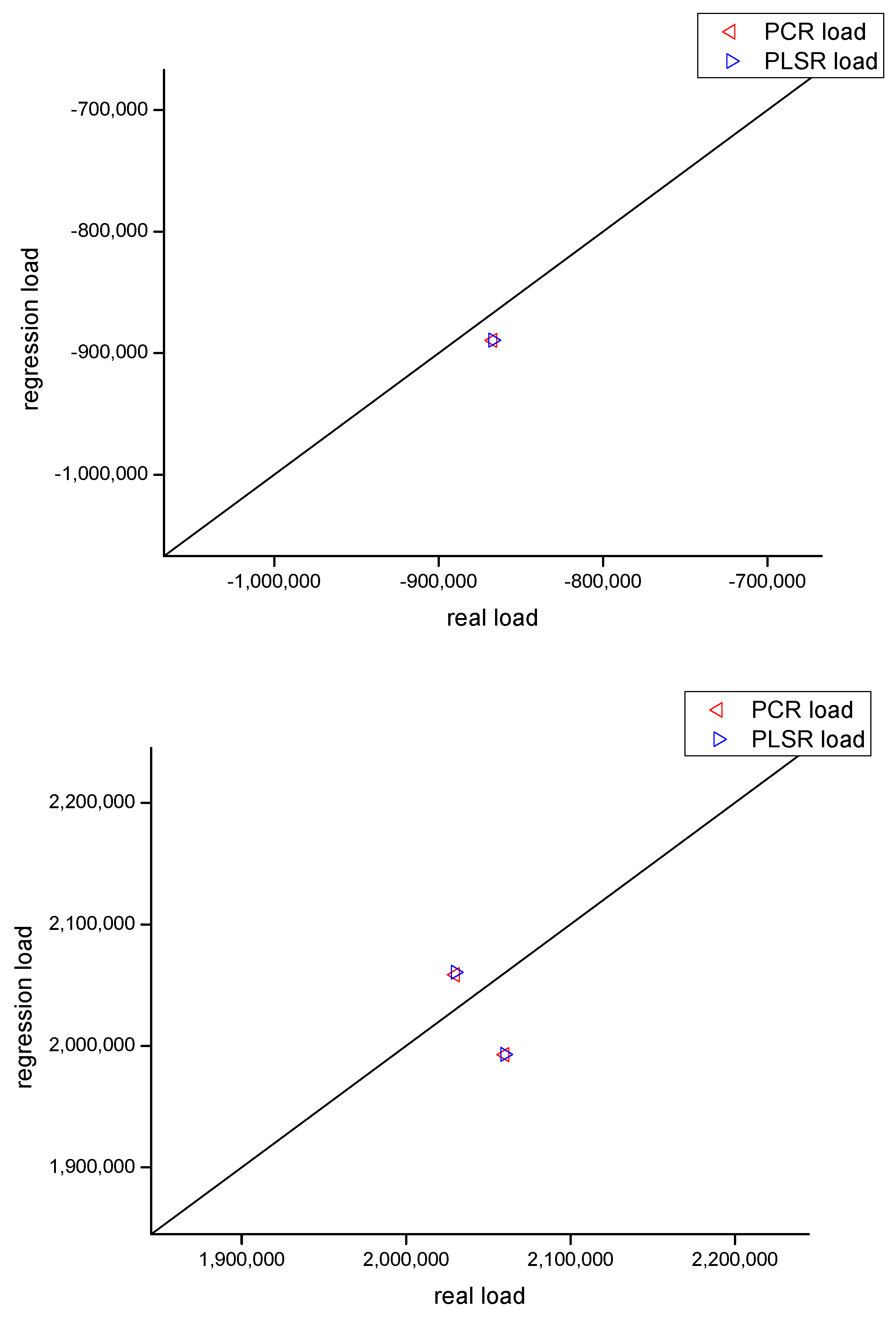
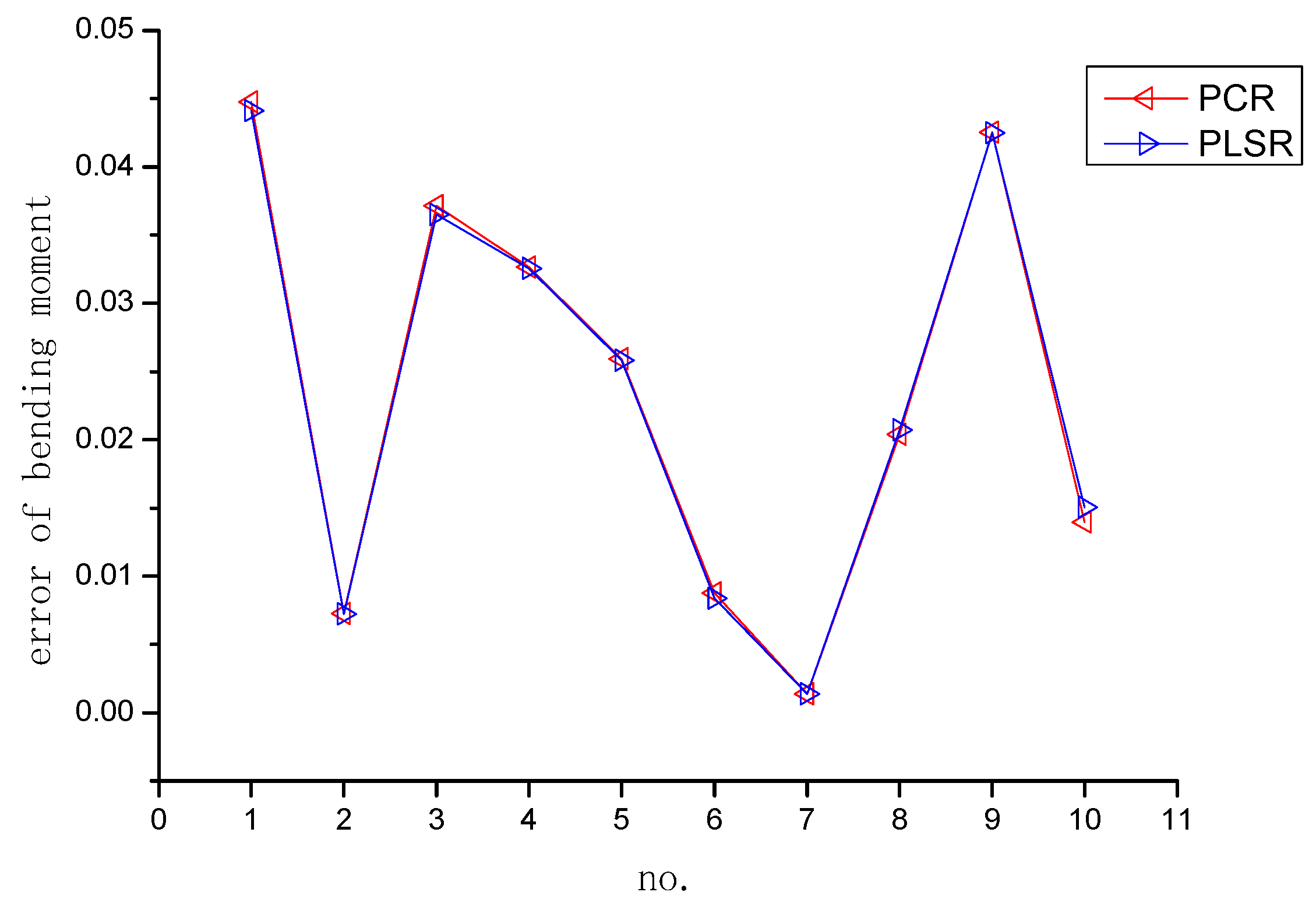
The regression results and real load are shown in Figure 5, Figure 6, Figure 7, Figure 8, Figure 9, Figure 10, Figure 11, Figure 12, Figure 13, Figure 14, Figure 15 and Figure 16.

Figure 5, Figure 6, Figure 7 and Figure 8 demonstrate the regression results of shear force, showing, respectively, the shear forces of different methods, a comparison between the real shear force and regression shear force, a detailed comparison between the real shear force and regression shear force, and the relative error of shear forces of different methods.

It can be seen that the regression shear forces are very close to the actual shear force, with all relative errors below 0.05 and most below 0.03. In comparison, the regression results of PCR and PLSR vary relatively. In some cases, the results of PCR are better than those of PLSR, while in others, the results of PLSR are better than those of PCR.

Figure 9, Figure 10, Figure 11 and Figure 12 demonstrate the regression results of bending moment, showing, respectively, the bending moments of different methods, a comparison between the real bending moment and regression bending moment, a detailed comparison between the real bending moment and regression bending moment, and the relative error of bending moments of different methods.

It can be seen that the regression bending moments are very close to the actual bending moment, with all relative errors below 0.05 and most below 0.04. In comparison, the regression results of PCR and PLSR vary relatively. In some cases, the results of PCR are better than those of PLSR, while in others, the results of PLSR are better than those of PCR.

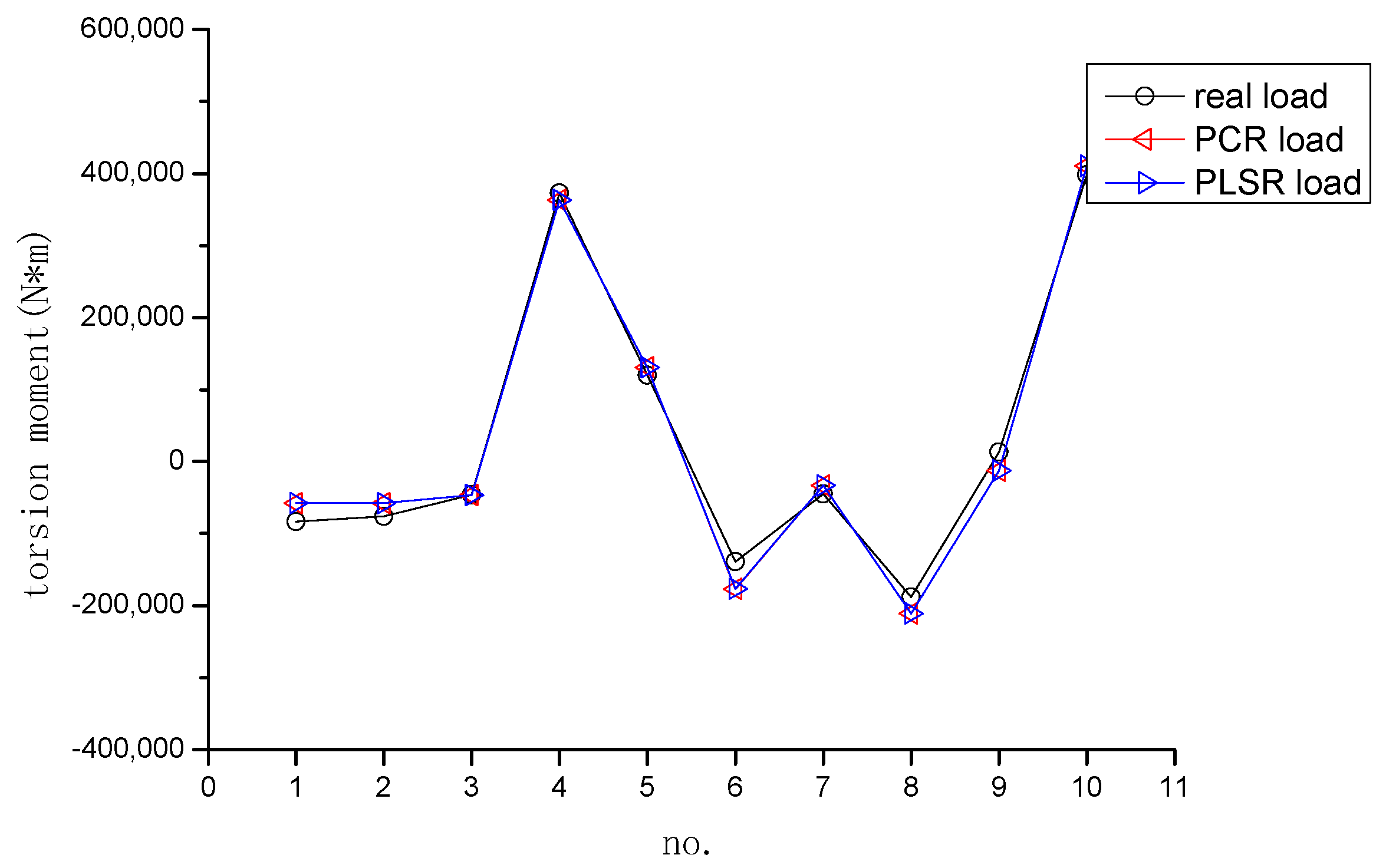
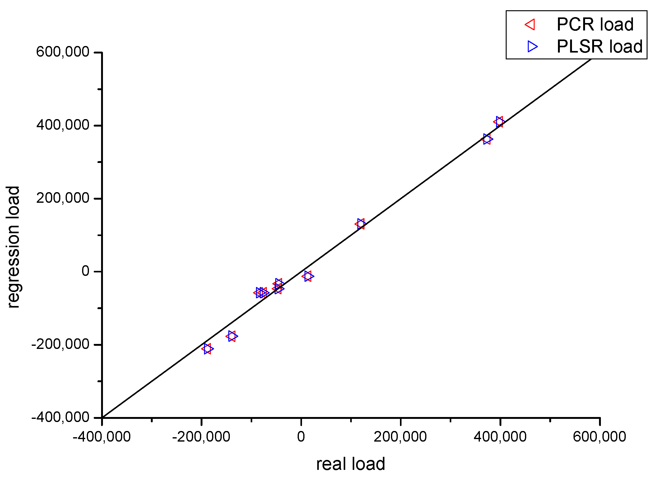
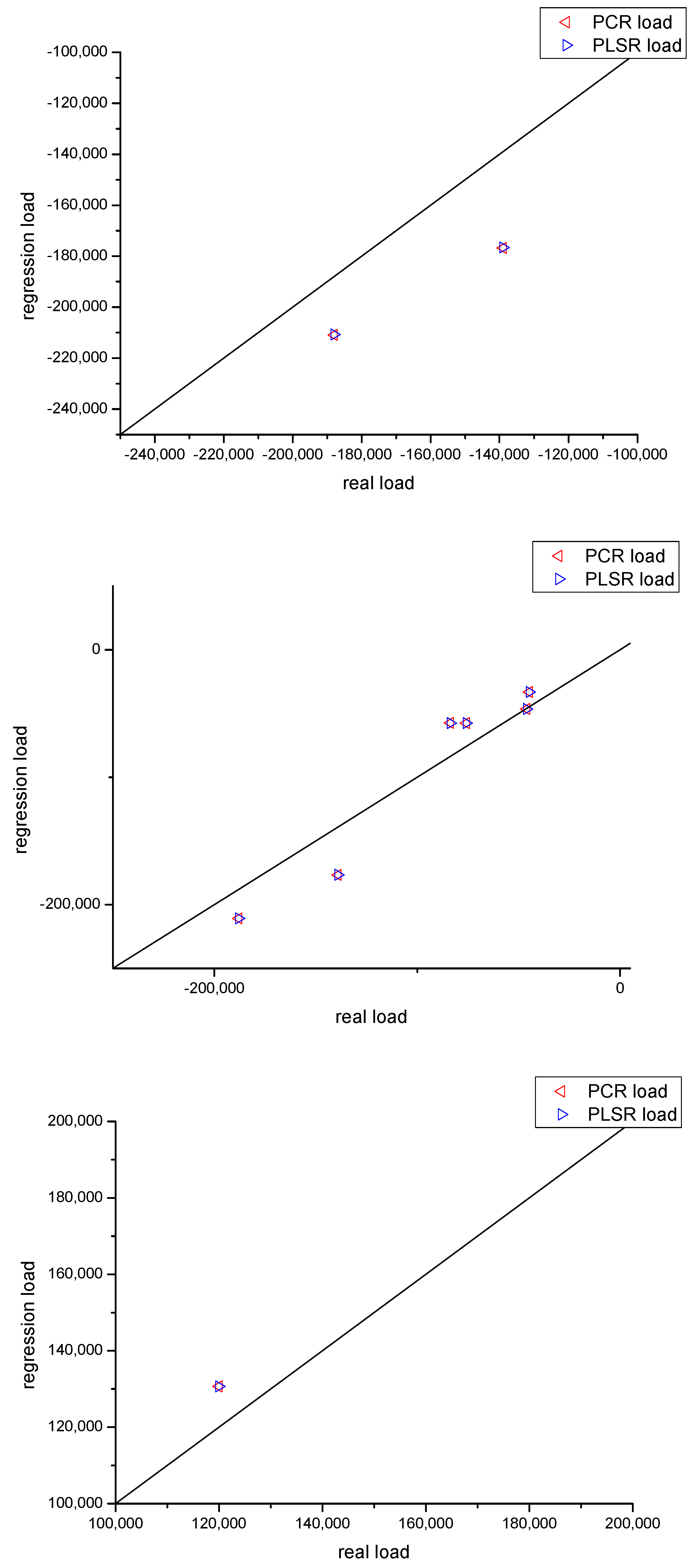
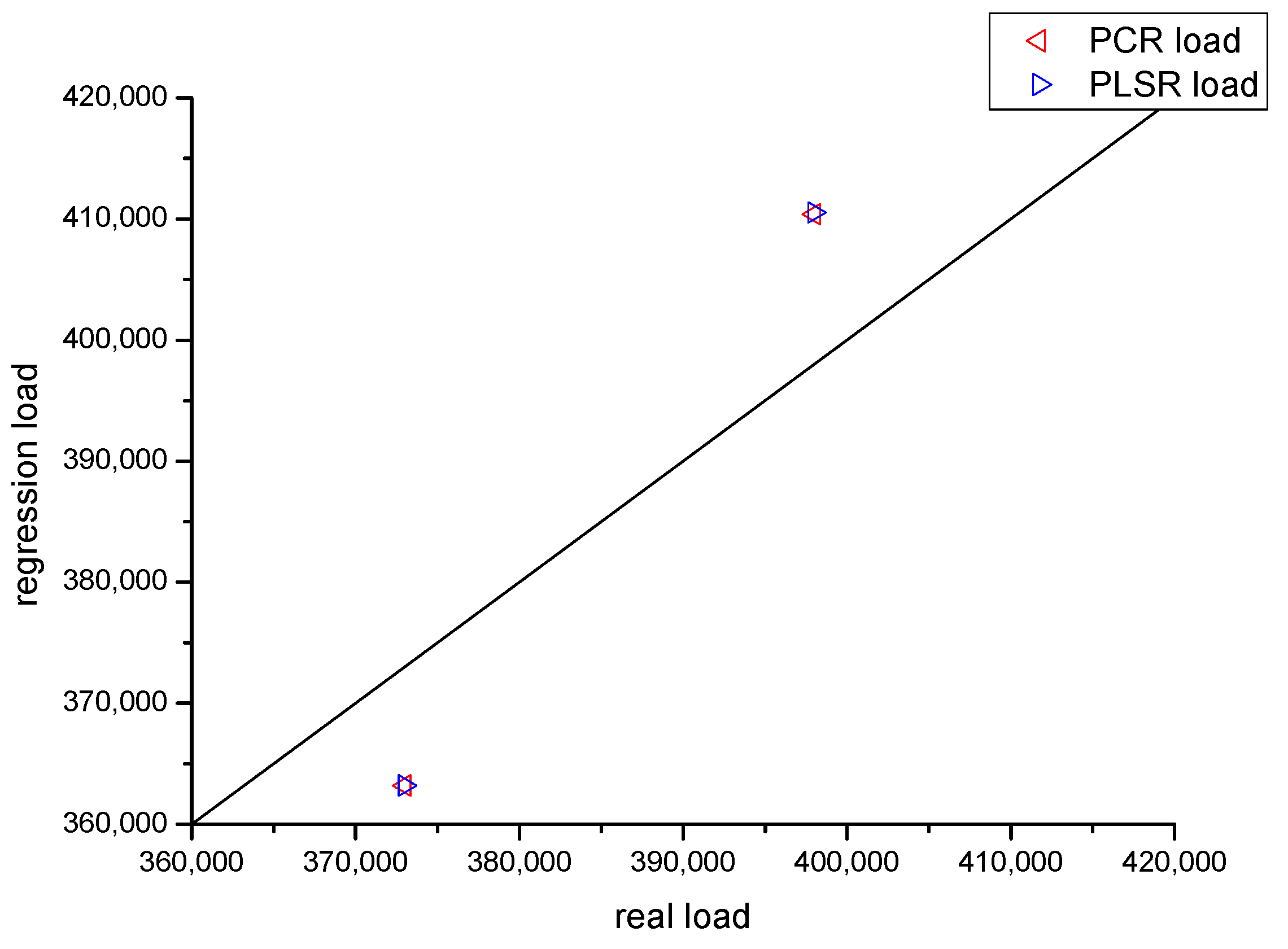
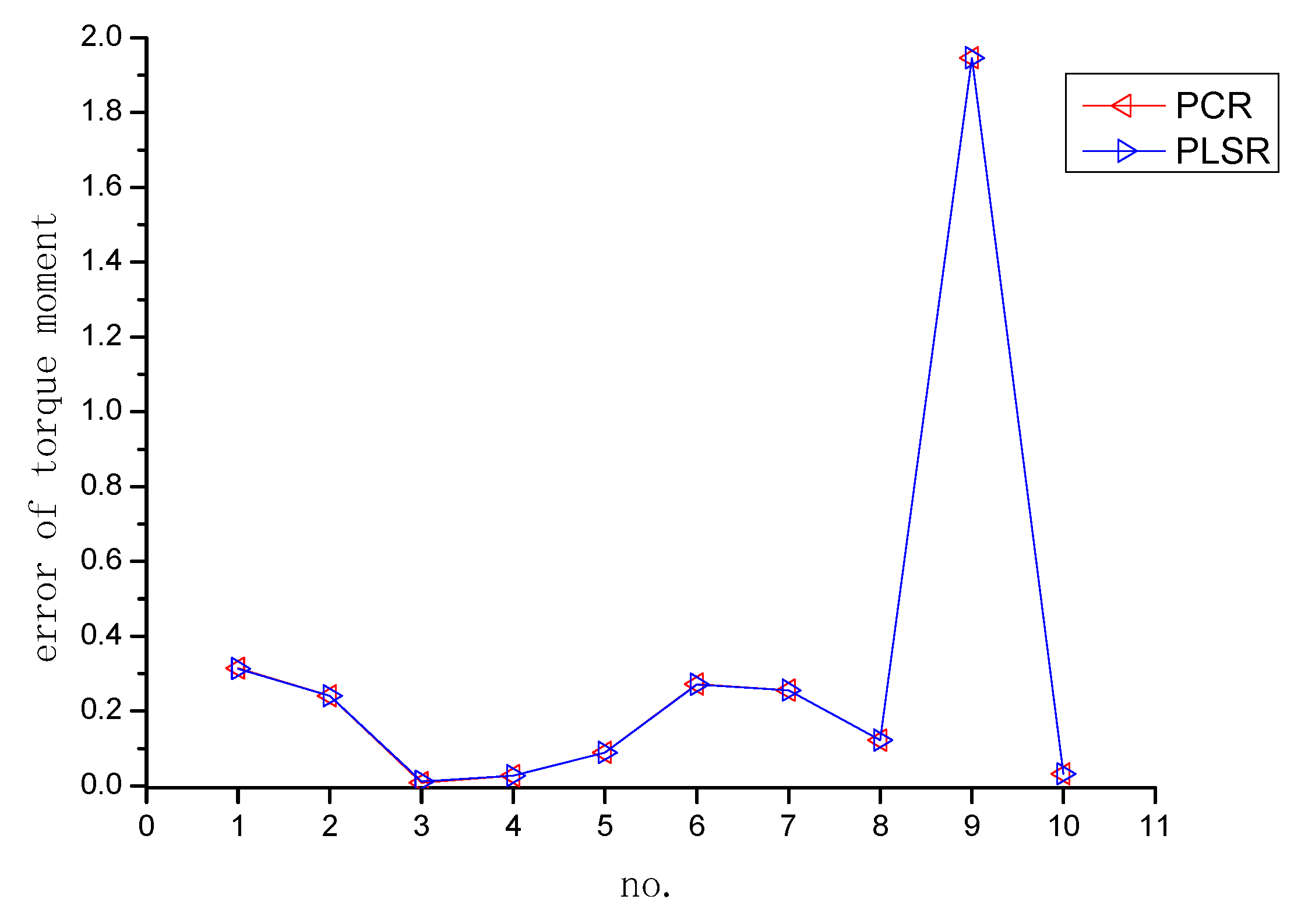
Figure 13, Figure 14, Figure 15 and Figure 16 demonstrate the regression results of the torque moment, showing, respectively, the torque moments of different methods, the comparison between the real torque moment and regression torque moment, the detailed comparison between the real torque moment and regression torque moment, and the relative error of torque moments of different methods.

It can be seen that the regression bending moments are close to the actual bending moment, with most relative errors below 0.3. In comparison, the regression results of PCR and PLSR are very close, and there is no apparent difference seen in the graph.

The detailed numerical comparison of the errors and relative errors of the regression results of PCR and PLSR is shown in

Table 3. Comparison between the real torque moment and regression torque moment.

No.	Real Load	PCR	PLSR	Error of PCR	Error of PLSR	Relative Error of PCR	Relative Error of PLSR
1	−8.4 × 104	−5.7 × 104	−5.8 × 104	2.6 × 104	2.6 × 104	0.31	0.31
2	−7.6 × 104	−5.8 × 104	−5.8 × 104	1.8 × 104	1.8 × 104	0.24	0.24
3	−4.6 × 104	−4.6 × 104	−4.7 × 104	3.7 × 102	5.1 × 102	0.01	0.01
4	3.7 × 105	3.6 × 105	3.6 × 105	9.8 × 103	9.8 × 103	0.03	0.03
5	1.2 × 105	1.3 × 105	1.3 × 105	1.1 × 104	1.1 × 104	0.09	0.09
6	−1.4 × 105	−1.8 × 105	−1.8 × 105	3.8 × 104	3.8 × 104	0.27	0.27
7	−4.5 × 104	−3.3 × 104	−3.3 × 104	1.1 × 104	1.1 × 104	0.26	0.26
8	−1.9 × 105	−2.1 × 105	−2.1 × 105	2.3 × 104	2.3 × 104	0.12	0.12
9	1.3 × 104	−1.3 × 104	−1.3 × 104	2.6 × 104	2.6 × 104	1.95	1.95
10	4.0 × 105	4.1 × 105	4.1 × 105	1.2 × 104	1.3 × 104	0.03	0.03

. In the table, the reason for the large relative error in the 9th case is that the numerical value itself is much smaller compared to other cases. Therefore, the calculated relative error is relatively large.

The MAE, MSE, RMSE, and R-square are shown in

Table 4. MAE of different methods.

	PCR	PLSR
Shear force	0.0190	0.0188
Bending moment	0.0235	0.0234
Torque moment	0.3304	0.3303

,

Table 5. MSE of different methods.

	PCR	PLSR
Shear force	0.0005	0.0005
Bending moment	0.0008	0.0008
Torque moment	0.4106	0.4103

,

Table 6. RMSE of different methods.

	PCR	PLSR
Shear force	0.0220	0.0217
Bending moment	0.0277	0.0276
Torque moment	0.6408	0.6406

and

Table 7. R-square of different methods.

	PCR	PLSR
Shear force	0.999512	0.999519
Bending moment	0.998976	0.998988
Torque moment	0.990028	0.990082

.

It can be seen that both PCR and PLSR have very good regression results, especially for shear force and bending moment, with MAE, MSE, and RMSE very close to 0 and R-square close to 1. The regression of torque moment is relatively poor, which may be due to the small numerical value of the torque moment, leading to a large relative error.

Comparing the results of PCR and PLSR, it can be observed that PLSR outperforms PCR in terms of MAE, MSE, RMSE, and R-square for all shear forces, bending moments, and torque moments. The improvements in the PLSR results can be attributed to the fact that PLSR takes into account the correlation between the response variables and the predictor variables, while PCR only considers the variance of the predictor variables.

In summary, the predictive accuracy of the flight load regression model based on PCR and PLSR constructed in this paper is very high and is able to meet the needs of flight load engineering applications. In particular, the regression effect of PLSR is slightly better than that of PCR.

By comparing various methods in

Table 8. Calculation time of different methods.

	PCR	PLSR	Panel method
Calculation time	0.0156s	0.0312s	>5 min × 10

, it becomes apparent that the computational time of regression models is significantly faster than that of panel methods, even with only 10 sets of operating conditions. If more datasets are calculated, the advantages of regression models will become even more apparent.

5. Conclusions

This study investigates the effectiveness of the flight load regression analysis method using PCR and PLSR. The results of numerical experiments demonstrate that the regression analysis based on PCR and PLSR achieves high accuracy. Through the analysis of various indicators, such as relative error, mean absolute error, mean square error, root mean squared error, and R-square between predicted values and true values for shear force, bending moment, and torque moment, it is confirmed that the regression analysis methods based on PCR and PLSR are suitable for flight load analysis, with PLSR slightly outperforming PCR.

Additionally, by adopting numerical analysis methods based on regression analysis, the need for complex finite element solving processes is eliminated, resulting in shorter solution times and improved computational efficiency. This provides an alternative approach for enhancing traditional flight load analysis methods.

In conclusion, the flight load regression analysis methods based on PCR and PLSR are applicable for predicting and analyzing flight loads while ensuring accuracy and significantly improving computational efficiency. Future research will focus on studying more complex flight conditions, such as roll maneuvering and yaw maneuvering, to achieve the rapid calculation of severe load scenarios within the flight envelope.

References

1. Acar, E.; Haftka, R.T.; Sankar, B.V.; Qiu, X. Increasing Allowable Flight Loads by Improved Structural Modeling. AIAA J. 2006, 44, 376–381. [Google Scholar] [CrossRef] [Green Version]
2. Kennedy, D.; Fischer, M.; Featherston, C.A. Recent developments in exact strip analysis and optimum design of aerospace structures. Proc. Inst. Mech. Eng. Part C J. Mech. Eng. Sci. 2007, 221, 399–413. [Google Scholar] [CrossRef]
3. Mani, M.; Dorgan, A.J. A Perspective on the State of Aerospace Computational Fluid Dynamics Technology. Annu. Rev. Fluid Mech. 2023, 55, 431–457. [Google Scholar] [CrossRef]
4. Fujii, K. Progress and future prospects of CFD in aerospace—Wind tunnel and beyond. Prog. Aerosp. Sci. 2005, 41, 455–470. [Google Scholar] [CrossRef]
5. Huang, M.; Wang, Z.-W. A Review of Wind Tunnel Based Virtual Flight Testing Techniques for Evaluation of Flight Control Systems. Int. J. Aerosp. Eng. 2015, 2015, 672423. [Google Scholar] [CrossRef] [Green Version]
6. D’Elía, J.; Storti, M.; Idelsohn, S. A closed form for low-order panel methods. Adv. Eng. Softw. 2000, 31, 347–353. [Google Scholar] [CrossRef]
7. Xu, H.; Huang, Q.; Han, J.; Yun, H. Calculation of Hinge Moments for a Folding Wing Aircraft Based on High-Order Panel Method. Math. Probl. Eng. 2020, 2020, 8881233. [Google Scholar] [CrossRef]
8. Yang, C.; Zhang, B.; Wan, Z.; Wang, Y. A method for static aeroelastic analysis based on the high-order panel method and modal method. Sci. China Technol. Sci. 2011, 54, 741–748. [Google Scholar] [CrossRef]
9. Li, H.; Zhang, Q.; Chen, X. Deep Learning-Based Surrogate Model for Flight Load Analysis. Comput. Model. Eng. Sci. 2021, 128, 605–621. [Google Scholar] [CrossRef]
10. Sykes, B.S.; Malan, A.; Gambioli, F. Novel Nonlinear Fuel Slosh Surrogate Reduced-Order Model for Aircraft Loads Prediction. J. Aircr. 2018, 55, 1004–1013. [Google Scholar] [CrossRef]
11. Lee, D.; Kang, Y.E.; Kim, D.; Yee, K. Aeroelastic Design and Comprehensive Analysis of Composite Rotor Blades Through Cluster-Based Kriging. AIAA J. 2022, 60, 5984–6004. [Google Scholar] [CrossRef]
12. Yan, Q.; Wan, Z.; Yang, C. Flight Load Calculation Using Neural Network Residual Kriging. Aerospace 2023, 10, 599. [Google Scholar] [CrossRef]
13. Kim, J.; Oh, Y.; Park, C.; Kang, Y.M.; Shin, H.; Kim, I.Y.; Jang, D.P. Comparison Study of Partial Least Squares Regression Analysis and Principal Component Analysis in Fast-Scan Cyclic Voltammetry. Int. J. Electrochem. Sci. 2019, 14, 5924–5937. [Google Scholar] [CrossRef]
14. Li, J.T.; Luo, Y.D.; Dai, H.L. Application of Principal Component Regression and Partial Least Squares Regression in Ultraviolet Spectrum Water Quality Detection. In Proceedings of the 2017 International Conference on Optical Instruments and Technology: Optoelectronic Imaging/Spectroscopy and Signal Processing Technology, Beijing, China, 28–30 October 2017; Volume 10620. [Google Scholar]
15. Ergon, R.; Esbensen, K.H. PCR/PLSR optimization based on noise covariance estimation and Kalman filtering theory. J. Chemom. 2002, 16, 401–407. [Google Scholar] [CrossRef] [Green Version]
16. Engelen, S.; Hubert, A.; Branden, K.V.; Verboven, S. Robust Pcr and Robust Plsr: A Comparative Study. In Theory and Application of Recent Robust Methods; Springer Nature: Berlin/Heidelberg, Germany, 2004; pp. 105–117. [Google Scholar]
17. Singh, M.; Sarkar, A. Comparative Study of the PLSR and PCR Methods in Laser-Induced Breakdown Spectroscopic Analysis. J. Appl. Spectrosc. 2018, 85, 962–970. [Google Scholar] [CrossRef]
18. Zhang, X.; Huang, B. Prediction of soil salinity with soil-reflected spectra: A comparison of two regression methods. Sci. Rep. 2019, 9, 5067. [Google Scholar] [CrossRef] [PubMed] [Green Version]
19. Polat, E.; Gunay, S. A simulation study for the comparison of two popular robust PLSR methods: RSIMPLS and PRM with a robust PCR method in the presence of outliers. In Proceedings of the International Conference of Numerical Analysis and Applied Mathematics 2014 (Icnaam-2014), Rhodes, Greece, 22–28 September 2014; Volume 1648. [Google Scholar]
Figure 1. Flowchart of loosely-coupled static aeroelastic analysis.
Applsci 13 08428 g001
Figure 2. Structure model of the plane.
Applsci 13 08428 g002
Figure 3. Aerodynamic model of the plane.
Applsci 13 08428 g003
Figure 4. Flowchart of panel method for flightload calculation.
Applsci 13 08428 g004
Figure 5. Shear forces of different methods.
Applsci 13 08428 g005
Figure 6. Comparison between the real shear force and regression shear force.
Applsci 13 08428 g006
Figure 7. Detailed comparison between the real shear force and regression shear force.
Applsci 13 08428 g007aApplsci 13 08428 g007b
Figure 8. Relative error of shear forces of different methods.
Applsci 13 08428 g008
Figure 9. Bending moments of different methods.
Applsci 13 08428 g009
Figure 10. Comparison between the real bending moment and regression bending moment.
Applsci 13 08428 g010
Figure 11. Detailed comparison between the real bending moment and regression bending moment.
Applsci 13 08428 g011aApplsci 13 08428 g011b
Figure 12. Relative error of bending moments of different methods.
Applsci 13 08428 g012
Figure 13. Torque moments of different methods.
Applsci 13 08428 g013
Figure 14. Comparison between the real torque moment and regression torque moment.
Applsci 13 08428 g014
Figure 15. Detailed comparison between the real torque moment and regression torque moment.
Applsci 13 08428 g015aApplsci 13 08428 g015b
Figure 16. Relative error of torque moments of different methods.
Applsci 13 08428 g016