Abstract
Ultra-wide-band (UWB) positioning is a satisfying indoor positioning technology with high accuracy, low transmission cost, high speed, and strong penetration capacity. However, there remains a lack of systematic study on inevitable and stochastic errors caused by factors originating from the multipath effect (ME), non-line-of-sight interference (NLOSI), and atmospheric interference (AI) in UWB indoor positioning systems. To address this technical issue, this study establishes a dynamic error-propagation model (DEPM) by mainly considering the ME, NLOSI, and AI. First, we analyze the UWB-signal generation principle and spread characteristics used in indoor positioning scenarios. Second, quantization models of the ME, NLOSI, and AI error factors are proposed based on data from related studies. Third, to adapt to various environments, we present a variable-weighted DEPM based on the quantization models above. Finally, to validate the proposed dynamic error-propagation model, UWB-based positioning experiments in an intelligent manufacturing lab were designed and conducted in the form of static and dynamic longitude-tag position measurements. The experimental results showed that the main influencing factors were ME and NLOSI, with a weight coefficient of 0.975, and AI, with a weight coefficient of 0.00025. This study proposes a quantization approach to main error factors to enhance the accuracy and precision of indoor UWB-positioning systems used in intelligent manufacturing areas.
1. Introduction
In general, positioning information can be provided by a global navigation satellite system (GNSS) [1] in outdoor usage for most moving objects. However, pure GNSSs cannot currently satisfy high-accuracy requirements in indoor positioning scenes because of the stochastic layout of shelters, obstacles, and the thick, metal roofs of workshops. In an indoor environment, different types of wireless positioning methods (e.g., Wi-Fi, ZigBee, and UWB) can be used to achieve relatively high-accuracy positioning. In practice, Wi-Fi positioning technology is realized in accordance with the intensity indication of signal reception [2]. Indoor positioning technology based on Wi-Fi signals has the advantages of a wide application range, low cost, and good portability [3]. However, external noise or other 2.4 GHz signals can easily interfere with Wi-Fi signals because of their limited transmission frequency bandwidth, leading to Wi-Fi positioning accuracy at the level of one meter. ZigBee wireless location technology was first introduced in 2002 [4]. However, the positioning accuracy based on ZigBee wireless positioning technology can reach only 1~5 m.
UWB was originally developed as a military radar and was mainly used in the radar field during its early stages. In general, UWB wireless positioning technology uses pulse signals with extremely low power spectral density and narrow pulse width to transmit data, achieving high time resolution and strong barrier penetration. In a line-of-sight (LOS) environment, centimeter- or even millimeter-level of positioning accuracy can be obtained [5,6,7]. In UWB-based positioning, typical location algorithms are classified as time of arrival (TOA), time differential of arrival (TDOA) [8], time of flight (TOF), received signal strength (RSSI), and angle of arrival (AOA) [9,10]. However, inevitable and stochastic errors are mainly caused by factors sourcing from the multipath effect (ME), non-line-of-sight interference (NLOSI), and atmospheric interference (AI) in UWB positioning systems. To address this technical issue, this study establishes a dynamic error-propagation model (DEPM) by mainly considering the ME, NLOSI, and AI.
Positioning error challenges exist in current intelligent manufacturing workshops. The location and trajectory information of each production element in the intelligent manufacturing workshop is basic for transparent production and the intelligent manufacturing operation control center. When UWB indoor positioning is carried out in an intelligent manufacturing workshop, there are many factors affecting the positioning results: (1) equipment. The number and location of UWB positioning devices can affect their positioning accuracy. (2) Occlusion. This can occur during the propagation of UWB positioning signals between base stations, and tag, refraction, diffraction, and other phenomena can occur when they are blocked by indoor objects, which will change the amplitude and phase of the signal and then produce positioning errors. (3) Time. The crystal oscillator frequency of each base station usually has a certain deviation due to the manufacturing process and its use in the experiment. (4) Environment. The state of the atmosphere at different times (temperature, pressure, humidity, etc.) can affect the propagation speed of UWB signal waves. (5) Software delay. When the processor analyzes the obtained data information, the software can delay, causing poor real-time positioning. (6) Moving the object with the UWB tag. When the UWB positioning tag is fixed on a moving object, an AGV, or worn by a worker, it is inevitable that shaking occurs during movement, resulting in a deviation in signal transmission [11,12].
The contributions of this study are as follows: (1) a dynamic propagation model of a UWB signal is established, and the factors that affect the UWB positioning accuracy are qualitatively analyzed. (2) Based on the previous study of the signal loss formula, quantization models of the multipath effect (ME), non-line-of-sight interference (NLOSI), and atmospheric interference (AI) error factors are proposed. (3) To adapt to various environments, a variable-weighted dynamic error-propagation model (DEPM) is presented based on the quantization models. (4) A cable UWB network in an intelligent manufacturing lab is designed to validate the proposed model.
The rest of this paper is organized as follows: In Section 2, we review related research concerning UWB signal propagation. In Section 3, we establish a UWB signal model to study the signal transmission mode and performance. In Section 4, we present a variable-weighted DEPM based on the quantization models of ME, NLOSI, and AI error factors. Section 5 describes static and dynamic positioning experiments conducted in an intelligent manufacturing lab, and the error weight is analyzed. In Section 6, we summarize the study and introduce future work.
2. Related Work
In 2002, the U.S. Federal Communications Commission allowed UWB carrier frequencies of 3.1~10.6 GHz for civil communication usage. The ratio of the −10 dB bandwidth to the system center frequency is larger than 20%, and the system bandwidth is at least 500 MHz [13]. The corresponding transmission power spectral density is less than −41.25 dBmW/MHz. Gaussian pulse waveforms are often used in UWB systems because they are easy to generate [14].
In the last decade of the 20th century, emerging ultra-wide-band (UWB) impulse technology was used in numerous applications in the commercial as well as the military sectors [15]. Table 1 lists the main methods in UWB positioning technology in the past decade undertaking various improved algorithms to improve positioning accuracy. D.P. Young et al. [16] explored the use of cross-correlation-based TDOA methods in conjunction with a novel technique for combining the TDOA estimates from multiple antenna pairs to build an estimate of the transmitter position. A. Subramanian et al. [17] proposed a distributed localization scheme for nodes with emphasis on power measurements (RSSI) using UWB. The localization algorithm was distributed and followed an indirect approach where nodes determine their location with the help of their neighbors. X. Yong et al. [18] applied an improved TDOA method to achieve UWB localization in the mobile environment. The ETDGE algorithm for ranging and the Fang iterative algorithm for locating the moving node were approached in an optimum manner.
In practice, the positioning accuracy of UWB systems always faces positioning error challenges caused by disturbance factors from ME, NLOSI, and AI. In the past decade, scholars proposed different error measurement algorithms and error elimination methods to address this issue. Typically, Cramer et al. [19] studied the joint TOA and AOA statistics of indoor UWB propagation channels, proposing an iterative UWB channel characterization algorithm, and the path loss characteristics of indoor UWB were studied using a Hermite polynomial model to simulate the received signals. Wang et al. [20] studied the path loss characteristics of indoor UWB systems using the spatial smoothing MUSIC algorithm to test the azimuth and elevation arrival angles of multipath signal challenges, determining that multipath reflection in small rooms was significantly higher than that in large rooms. Cimdins et al. [21] proposed a multipath-assisted deviceless localization system with amplitude and phase information that calculated the influence on the received signal based on the position of the person in the target area. Liu et al. [22] proposed a practical NLOS recognition technique, including a reduction factor to reduce the severe impact of NLOS situations and a set of appropriate features to improve the speed of NLOS recognition. Spencer [23] considered the AOA based on the Saleh–Valenzuela model and verified the effectiveness of using a spectrum to overcome the ME. Ershadh et al. [24] studied a new modeling method for parameter estimation of low-level multipath structures in UWB indoor communication channels. This method reduced the lack of transparency in the entire parameter estimation process and optimized the performance evaluation of the UWB physical layer scheme. Mosbah et al. [25] proposed a proportional adaptive technology to alleviate the multipath fading effect in advanced wireless communication systems. Hua et al. [26] proposed a multipath map based on the principle of spatial domain modeling. Su et al. [27] adopted a beam-guided circularly polarized antenna to suppress indoor multipath propagation. Feng et al. [28] put forward an indoor positioning system (IPS) combining inertial measurement unit (IMU) and UWB, which improved the robustness and accuracy of the system through extended Kalman filter (EKF) and unscented Kalman filter (UKF). Zhao et al. [29] studied an algorithm based on RSS residual weighting (RRW) to alleviate the line of sight nonlinearity and reduce positioning errors.
In addition, some auxiliary sensors, such as IMUs, lidar, and R-GBD cameras, can be used in UWB systems to improve positioning accuracy. Liu et al. [30] proposed an adaptive complementary Kalman filter method to perform fusion filtering on UWB and IMU data and track errors in variables, such as position, speed, and direction, which not only eliminates the ME but also corrects the deviation of velocity and acceleration caused by IMU drift. Liu et al. [31] proposed a pedestrian indoor positioning method based on a UWB and a visual fusion algorithm. By combining the two sensors, the scale ambiguity of monocular circular simultaneous localization and mapping (SLAM) was solved, and the UWB positioning accuracy was improved by relocating the failed visual trajectory through the UWB system.
Song et al. [32] combined UWB and two-dimensional LIDAR sensors to provide a more accurate and comprehensive image of the surrounding environment. Alternatively, UWB ranging can eliminate the accumulated error based on a LIDAR–SLAM algorithm. Koppanyi et al. [33] used a UWB- and IMU-integrated navigation system based on adaptive motion constraints to solve the short interruption problem of UWB systems. Yang et al. [34] combined the UWB with ultra-high time resolution, good anti-multipath ability, and strong penetration ability, as well as the active composition and positioning ability of LIDAR, to improve positioning accuracy. Li et al. [35] used a tightly coupled GPS–UWB–IMU navigation system based on an improved robust Kalman filter for better positioning accuracy. Fan et al. [36] introduced an antimagnetic ring to eliminate outliers of a UWB system in an NLOS environment and integrated inertial navigation system (INS) attitude information. Kok et al. [37] studied an tight-coupling IMU–UWB accurate positioning system to obtain accurate position and orientation estimates.
In summary, positioning accuracy is the most important performance parameter used in indoor wireless positioning systems, compared with precision, complexity, scalability, robustness, and cost. The mean distance error is adopted as the performance metric, which is the average Euclidean distance between the estimated location and the true location. However, location precision addresses how consistently the system works. The cumulative probability functions of the distance error can be used to measure the precision of a UWB-based positioning system [38]. Therefore, this study focuses on a dynamic error propagation model for accuracy performance.

Table 1.
Main methods in UWB positioning technology.
Table 1.
Main methods in UWB positioning technology.
| No. | Author/Year | Model and Algorithm | Quantization | Application Scenarios | Data Sources |
|---|---|---|---|---|---|
| 1 | D.P. Young, 2003 [16] | (a) Cross-correlation-based TDOA. (b) TDOA estimates from multiple antenna pairs. | Weighting functions | An unfinished 13 m wide, 20 m deep, and 12 m high anechoic chamber. | Simulated |
| 2 | A. Subramanin, 2005 [17] | (a) Nodes determine their location with the help of their neighbors. | Average mean and standard deviation | A simulation software: Glom-Mosim. | Simulated |
| 3 | Xu Yong, 2006 [18] | (a) ETDGE ranging algorithm. (b) Fang iterative locating mobile node algorithm. | Ranging error and average positioning error | Low-rate UWB communication systems in the mobile environment. | Numerical Simulation |
| 4 | M. Kok, 2015 [37] | (a) IMU combined with UWB. (b) Solve the maximum posterior problem. | Orientation and position estimation | Clock deviation occurs in UWB. | Physical Experiment |
| 5 | Z. Koppanyi, 2018 [33] | (a) An adaptive constraint used in the navigation filter. (b) IMU-detecting neural networks to determine the current dynamic state. | 10–30% (10–15 cm) improvement for 5–10 s long outages. | Unexploded ordinance mapping platform. | Experiment |
| 6 | C. Hua, 2020 [26] | (a) Spatial domain modeling principles of multipath mapping. (b) Improved nonlinear iterative algorithm with height component constraint. | Root-mean-square error, mean absolute error, and standard deviation | For a different indoor environment and layout of base stations. | Experiment |
| 7 | D. Feng, 2020 [28] | (a) The relationship between base station geometric distribution and base station precision factor. (b) UWB combine with IMU. | Root-mean-square error and CDF | Complex environment positioning. | Simulated and Experiment |
| 8 | K. Zhao, 2020 [29] | (a) An M/N-K sliding window to determine the loading and unloading of goods. (b) NLOS error is reduced based on RSS residual weighting. | Root-mean-square error and CDF | The intelligent warehousing management system. | Simulated and Experiment |
| 9 | M. Cimdins, 2020 [21] | The pulse response measurement of the UWB channel extracts multiple multipath components. | Mean localization error and ECDFs | The probability of position error in an indoor environment system is known. | Simulated |
| 10 | M. Ershadh, 2021 [24] | Estimation of the parameters of the underlying multipath structure in UWB indoor propagation channel. | Multipath parameters estimation | NLOS and LOS scenarios. | Simulated |
| 11 | Authors in this study | Dynamic error-propagation model used in UWB indoor positioning considering the multipath effect and atmospheric interference. | Root-mean-square error | Manufacturing production line. | Simulated and Experiment |
3. UWB Signal Propagation Properties
UWB wireless communication systems transmit information by large amounts of short and fast energy pulses. The allowed civil communication usage should be in the frequency band of 3.1~10.6 GHz. The corresponding transmission power spectral density must be less than −41.25 dBmW/MHz [13,14,39]. As described in Equation (1):
where and represents the lower limit and upper limit of frequency, respectively, when the peak power drops 10 dB; and represents the center value of the upper and lower frequencies of the carrier.
3.1. UWB Signal Generation
Before introducing the UWB signal, a Gaussian pulse signal is introduced because of its advantages in terms of time response, frequency response, and signal-to-noise ratio [40]. Its one-dimensional form is
where σ2 denotes the variance of the Gaussian pulse signal. To simplify Equation (1), we set α2 = 4πσ2. Then, the time-domain expression of the Gaussian pulse is
where α denotes the forming factor of the Gaussian pulse. By tuning the forming factor α, narrow pulses of different pulse widths can be obtained. The larger the value of α, the wider the pulse width, and the narrower the corresponding spectrum. Reducing the value of α compresses the pulse width, thus expanding the bandwidth of the transmission signal. The Gaussian pulse waveform with amplitude normalization is shown in Figure 1.
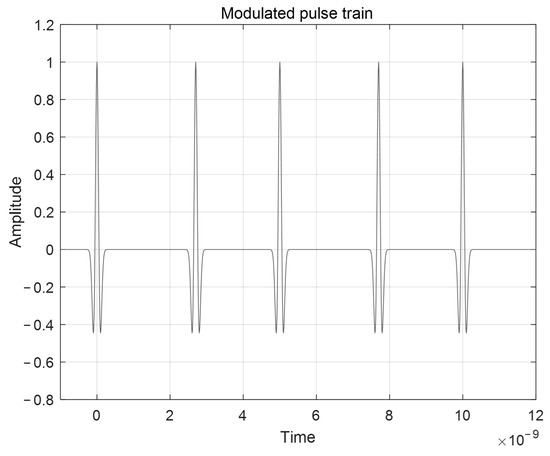
Figure 1.
UWB signal transmitting simulation.
In the UWB positioning system, to transmit the signal, the second or higher derivative of the Gaussian pulses is typically adopted in the signal transmission block diagram shown in Figure 2. The second-order derivation is
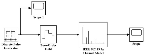
Figure 2.
Signal transmission block diagram. Scope1: signal by the sender, Scope: received signal by the receiver.
3.2. Temporal and Spatial Propagation of UWB Signals
In general, the performance of a wireless communication system depends on the characteristics of the channel. The UWB communication channel is only made between the signal sender and receiver. During the signal propagation, the direction of signal propagation will be shifted with an offset due to the obstacles. The signals at the receiver are the superposition of multiple signals, and the time of signal arrival and propagation path are different, which will also lead to changes in the phase and amplitude of the signals at the receiver. Therefore, it is necessary to establish a reliable UWB channel model. In fact, the UWB channel can be regarded as an open loop control system, as shown in Figure 2. The given transmitted signal is the input, and the received signal is the output [41].
UWB channels are divided into four types according to four typical channel conditions, CM1, CM2, CM3, and CM4, as shown in Table 2. Figure 3 shows the UWB transmitting signal, and Figure 4, Figure 5, Figure 6 and Figure 7 show receiving signal among CM1~CM4 channels, respectively, in which the Y-axis represents the amplitude of the normalized UWB signal. The amplitude gain can be calculated as
Table 2.
Four typical channel conditions.
Figure 3.
UWB Transmit signals. LOS means line-of-sight, and NLOS means non-line-of-sight.
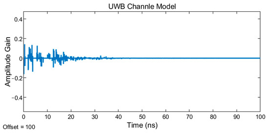
Figure 4.
UWB signals received after indoor multipath CM1 fading.
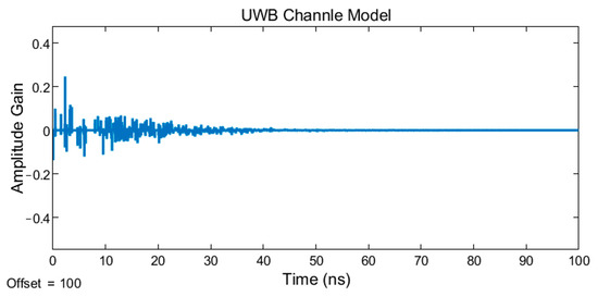
Figure 5.
UWB signals received after indoor multipath CM2 fading.
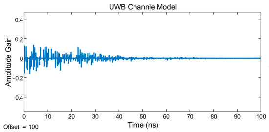
Figure 6.
UWB signals received after indoor multipath CM3 fading.
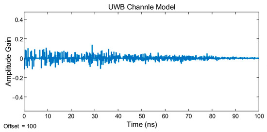
Figure 7.
UWB signals received after indoor multipath CM4 fading.
4. Dynamic Error Propagation Model in UWB-Based Positioning
4.1. UWB Signal Generation
The amplitude of the received UWB signal decreases greatly with time after indoor path loss. When the obstacle blocks the signal diameter propagation between the UWB tag and the base station, the signal amplitude of the first path will suffer serious losses, which is called non-line-of-sight (NLOS) propagation. In NLOS, there is a time delay, which is denoted as τ. The distance will be bigger than the actual distance because of the time delay τ. In the indoor environment, UWB signals are prone to be affected by different types of obstacles during signal transmission, resulting in a non-linear transmission phenomenon.
Most of the research shows that the indoor path loss follows a logarithmic path distance loss model:
where represents the signal loss in the line-of-sight (LOS) case, γ denotes the loss index, and denotes the reference distance. is defined as:
where f1 and f2 represent the frequencies in the radiation spectrum at the −10 dB edge. denotes the signal loss under NLOS conditions.
The phenomenon that causes signal superposition is called the multipath effect. As shown in Figure 8, a signal is transmitted along the direct path(black line) from Node 1 to Node 2, and it’s refracted signal is also transmitted along two possible reflection paths(red or blue dash lines) to Node 2—if the signal is superimposed in the same direction, multipaths have little effect on the decoding of the signal. However, if the length of the two paths is exactly half a wavelength apart at this point, then the two signals eliminate each other exactly when they reach Node 2, which distorts the signal and prevents the receiver from decoding the signal.
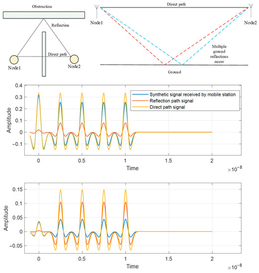
Figure 8.
Reflection model of UWB signal propagation.
According to the analysis above, the multipath effect is finally reflected in the superposition of signals under different paths. Signals received from different paths have been subjected to path loss and shadow fading in the propagation process. If a uniform line array is adapted to receive at the receiving terminal, the received signal is as follows [42]:
where is the amplitude; is the angle of arrival; is a time delay; is an array element; is the ith transmitting signal; is the speed of propagation; is the spacing of an array element; is the number of information sources; is the number of multipath components in a cluster; is the Gaussian white noise whose mean value, which is 0; and the power spectrum is .
4.2. Errors Caused by Atmospheric Interferences
In general, UWB wireless communication signals can be disturbed by the atmosphere during their propagation. The ranging distance D that accounts for atmospheric interference conditions can be calculated as [43]
where c denotes the speed at which light waves travel in a vacuum; t denotes the propagation time of the signal between the transmitter and receiver; and n = f(T,P,E,λ) in which T denotes the temperature, P denotes the air pressure, E denotes the humidity, and λ denotes the mean value of the signal wavelength.
To a certain extent, T, P, and E will affect the transmission of light speed in the form of electromagnetic waves, which normally travel in a straight line, and are deflected by changes in atmospheric conditions as they pass through the atmosphere.
The refractive index of the atmosphere, , under standard atmospheric conditions can be calculated as [44],
According to the arbitrary calculated under atmospheric conditions , the atmosphere refractive index is then
where α denotes the coefficient of air expansion. According to the experimental description in the literature [44], under environmental conditions of temperature = 21 °C, relative humidity = 71%, and atmospheric pressure = 101.325 kPa, the error caused by the atmospheric refractive index can be calculated approximately at the centimeters level and increases with the observation distance.
4.3. Dynamic Error Propagation Model
In UWB positioning, the signal attenuation caused by multipath and NLOS is reflected in the unsteadiness of the time delay of a received signal. Assuming that the channel delay is τ, the measuring distance is . The range under multipath and NLOS interference are
where dmea is the measured distance. Then, we define the error caused by ME and NLOSI as
where drea is the real distance between a UWB tag and the corresponding base station. To obtain the ground truth value of drea, we used a professional laser instrument, Fluke 410, with ranging of 0.2~100.0 m, an accuracy of 2.0 mm, to measure as an absolute reference value of drea. We use this laser rangefinder to measure static longitude UWB tags to the global coordinate origin. The location of the base station is fixed. When the position of each base station is known (measured with the laser rangefinder Fluke 410 in this study), the real distance information between the tag and the base stations can be obtained by using the distance Equation (9).
For the ME model, if EME,NLOSI is the multipath error, we can introduce eME,NLOSI by normalizing EME,NLOSI as follows:
where eME,NLOSI is a Gaussian random variable with mean value mME,NLOSI and variance σME,NLOSI in [45], and the explanation of log(1 + d) can be obtained in reference [46].
where d is the radial distance from the positioning point. AI is mainly caused by the refractive index of air in the atmosphere, which is affected by atmospheric conditions, such as temperature and humidity. Here, partial derivatives of P, E, and T can be obtained, respectively, to analyze each influencing factor.
By introducing in Equation (9), the equations above can be reorganized as
The atmospheric error can then be modeled as
In reference [46], the ranging accuracy was compared on a 10 km baseline. The results confirmed that the ranging error caused by the atmospheric medium was 0.25~0.75 m even if a high-accuracy electromagnetic wave rangefinder was adopted. Therefore, we lineally calculated the error caused by the atmosphere within a 10 m indoor space is defined as 0.25~0.75 mm.
To adapt a specific environment with corresponding ME–NLOSI and AI error factors, we introduce the two weights and to describe their impact ratios to the total positioning error, respectively. Further, the variable-weighted error propagation model of a UWB indoor positioning system can then be calculated as
where is the dynamic error propagation model. These weights should be variable to adapt to the different environments including the layout of production lines, obstacles blocking the UWB signals, and atmospheric conditions. Therefore, weights and . should be calibrated in a new environment.
5. Case Study
5.1. UWB Positioning System Design
In this study, the functional structure of the UWB positioning system is designed, as shown in Figure 9. The architecture of a complete positioning system in a workshop can be divided into four layers, perception, transport, analysis, and service, as shown in Figure 10. Each layer plays a relatively independent role in the positioning system. The perception layer is the sensing process of UWB signal sending to receiving. Before the base station communicates with the label, the respective parameters need to be configured to guarantee desired positioning results. The transmission layer is data transmission between the base station and the server, which can be realized through the wire, the base station and PC are connected to the transport layer and the service layer. The service layer includes a UWB location server, which visualizes the resolved location data through UWB location engine software.
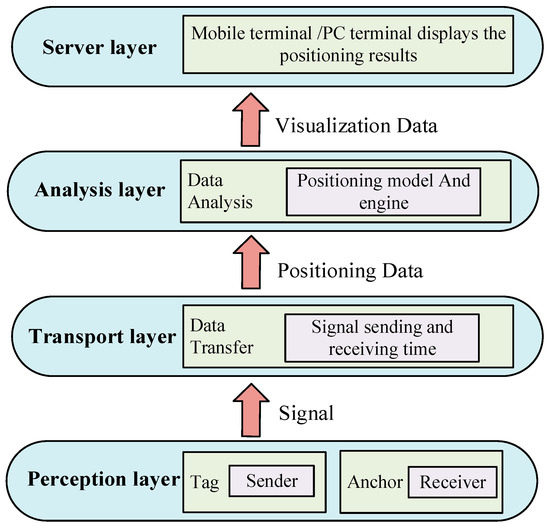
Figure 9.
The functional structure of a UWB positioning system.
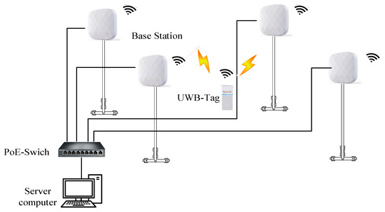
Figure 10.
The hardware topology of the UWB positioning system.
As the hardware topology of the UWB positioning system is shown in Figure 10, the POE switch can realize the transmission of positioning data in the same network. The main implementation of the analysis layer is to parse the internal hexadecimal message through the server, including the time of sending and receiving data, transmission frequency, etc.
5.2. Experiment Environment
To validate the dynamic error-propagation model proposed above, four base stations (as shown in Table 3), marked as BS1, BS2, BS3, and BS4, are set up in a 10 m × 10 m area (humidity 67%, temperature 15 °C, pressure 100 kph in the current environment) as shown in Figure 11. The base station IDs, respectively, are BS1:00003109, BS2:0000313f, BS3:000030f2, and BS4:000030f. The coordinates of the base station are BS1 (120,300,220), BS2 (420,300,220), BS3 (120,540,220), and BS4 (420,540,220). The unit is cm, with the lower corner of the right front as the origin of coordinates O (0,0) in the signal coverage area, calibrating UWB-Tag position at nine static points (T1, T2, …T9). Coordinate information is provided in Table 4.
Table 3.
Hardware configuration in UWB positioning system.
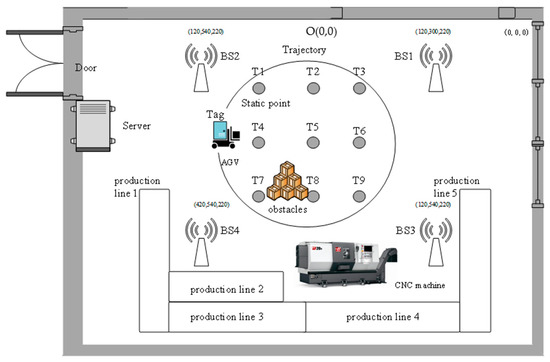
Figure 11.
UWB positioning of AGV on a production line in an intelligent manufacturing lab. Note, T1, T2, …T9 are the static points used for UWB-tag position calibration in this lab.
Table 4.
UWB-Tag layout in position calibration.
5.3. Measurement of Atmospheric Parameters
As shown in Figure 12, we built an atmosphere parameter sampling system, consisting of integrated sensor hardware and software.
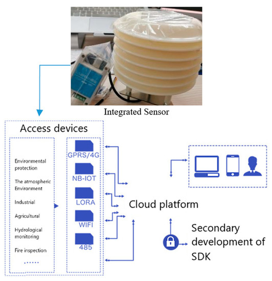
Figure 12.
The atmosphere parameter sampling system consists of sensor hardware and cloud software.
In fact, we use the temperature and humidity sensor to measure the actual atmospheric state and transmit the measured value onto a cloud server through the RS-485 field bus converter. The calibration process is conducted by this atmosphere sampling system shown in Figure 13. Generally, after a 2–3 s self-calibration process, the output of the measured sensor is the absolute value that meets the positioning requirements. Therefore, this study does not involve redundant calibration work.
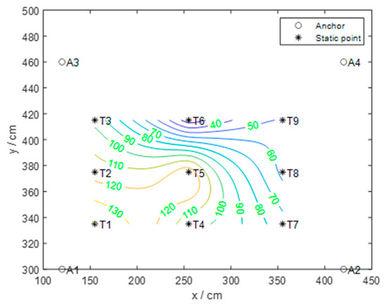
Figure 13.
The error distribution of intelligent manufacturing experiment production lines. Note, T1, T2, …T9 are the static points used for UWB-Tag position calibration in this lab.
5.4. Experiment Results
5.4.1. Measured Error Distribution
As can be seen from the measured error distribution in the form of a heat map, the maximum deviation in this area is 1.4 m, located at static label T1, and the minimum deviation is 0.22 m, located at static label T6 in Figure 13 and Figure 14. The average positioning error in this environment is 0.78 m. The reason for the small error in the center of the region is that the static points here can receive signals from the four base stations evenly. However, the positions with large error values are generally distributed near obstacles and base stations. First, the blocking of obstacles leads to interference in signal transmission. Secondly, the static point close to the base station cannot accurately receive the signal from the base station farther away.
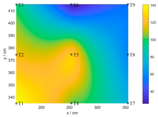
Figure 14.
Heat map of intelligent manufacturing experiment production line positioning error. Note, T1, T2, …T9 are the static points used for UWB-tag position calibration in this lab.
5.4.2. Atmospheric Error
The ranging accuracy of 10 km baselines is referred to in reference [46]. The results showed that the ranging error caused by atmospheric medium is between 0.25 m and 0.75 m even with the high precision electromagnetic wave rangefinder. In this experiment, the launch distance between the base stations is 0~4 m. According to the latest national standard specification of the atmosphere, temperature, pressure, and humidity, these factors’s variation with distance can be obtained in Matlab 2020b, as shown in Figure 15. The scattered points are the actual values measured by the sensors, and the straight lines are the atmospheric conditions obtained by theoretical fitting. It can be found that the range of temperature change is 0.02 °C, the range of air pressure change is 0.4 kph, the range of humidity change is 0.02%, and the range of atmospheric refractive index change is 0.00003%. According to Equation (11), the relation between the refraction error and the distance within 4 m is obtained, and the error range is 0.24 mm, as shown in Figure 16.
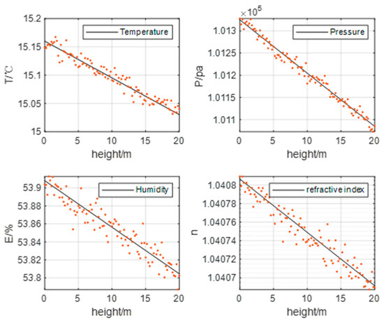
Figure 15.
Changes in indoor temperature, air pressure, humidity, and atmospheric refractive index from 0~4m.
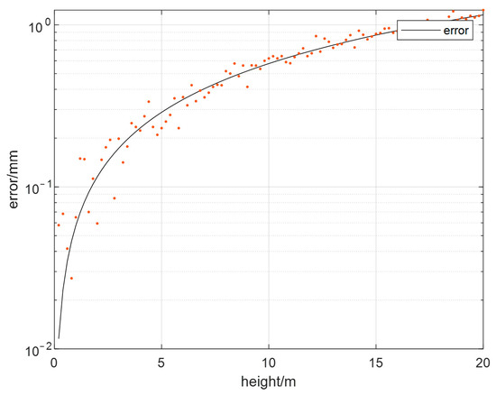
Figure 16.
The relation between 0~4 m distance and refraction error.
5.4.3. Dynamic Experiment and DEP Model
In the area covered by the signal, the UWB tag is fixed on an AGV on a production line in an intelligent manufacturing lab in Figure 11. The ID of the tag is DAF3, and the distance of the automatic guided vehicles (AGV) is set at 10 m. The positioning results of the trolley after walking are shown in Figure 17. Interference from various metal obstacles and the walking of stuff or movement of AGV demonstrated a significant impact on positioning accuracy. The maximum deviation was 1.6 m.
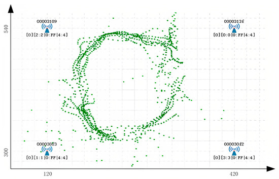
Figure 17.
UWB positioning results (horizontal axis unit: cm; vertical axis unit: cm).
In an independent UWB positioning experiment, errors of , , and the final error of were measured in Figure 18. Then, we repeated this experiment fifty times in the same environment as the lab. Further, we calculated the error weights and in the DEP model using the mean measured errors and based on these fifty experiment results. The final data show that the main influencing factors were the multipath effect and non-line-of-sight, with weight a coefficient of 0.975. However, the weight coefficient of atmospheric interference accounted for only 0.00025.
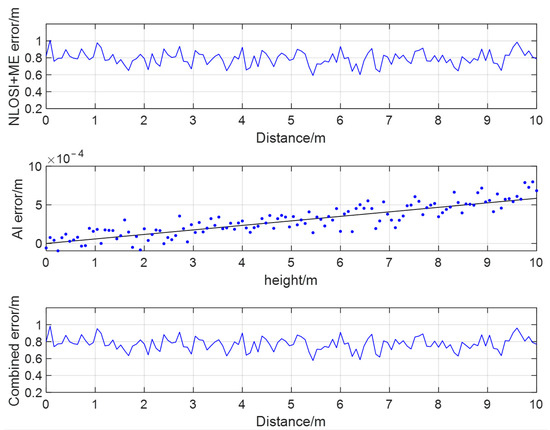
Figure 18.
Measured results of three errors in UWB error dynamic propagation. Note, the blue dots are the measured AI error values of the experimental UWB location system, and the black line is the fitted line of these blue dots.
The multipath effect (ME), and non-line-of-sight interference (NLOSI) in Figure 18 were obtained by MATLAB calculation based on the measured data in an experiment. The atmospheric interference (AI) was obtained by MATLAB simulation according to reference [46]. The three errors were accumulated and summed based on variable weights, and the total error is calculated according to Equation (21).
5.4.4. Discussion
The sum of the two types of error weight coefficient is 0.97525. We should pay attention to the fact that this sum is not equal to 1 because this study only considers multipath effects, NLOS transmission, and atmospheric disturbances, and not all interference factors. In fact, there exist other types of interferences in indoor environments, such as the time between UWB equipment [14] asynchronies, etc., which are not considered in this study. Furthermore, Figure 13 and Figure 14 indicate that the maximum deviation in the experiment area is 1.4 m, which is considered high for most UWB systems. The dynamic error propagation model did not improve the positioning accuracy, therefore, 1.4 m in the experiment was only used to analyze the weights of all the error factors.
Focusing on the weights of the positioning position error, it can be found that compared with the multipath effect and non-line-of-sight propagation, atmospheric interference has a very small proportion of the influence value on the total error. However, it is still significant for the quantization impact of atmospheric interferences on the total positioning error, which was completed in this study. In an intelligent workshop, chemical workshop, textile workshop, and other indoor environment with a large amount of dust and other particles, floating and sediment in the air will have a great impact on the signal refractive index, which should be included according to this DEP model in this study.
In fact, the error weight determination depends on environmental conditions and the layout of the obstacles, on the lab experimental data. The coefficients are constant after calibration in a given environment. Further, the weight coefficient under different scenarios should be calibrated again in each new environment.
6. Conclusions
In this paper, we proposed a variable-weighted error propagation model of a UWB indoor positioning system in an intelligent manufacturing lab quantitatively. First, we introduced the working principle and propagation characteristics of UWB signals. The ME, NLOSI, and AI were quantitatively analyzed to establish a DEP model. The weight relationships were then obtained through a case study in lab experiments. Based on the experimental results, we found that the main factors leading to inaccurate positioning of the UWB system were ME and NLOSI. Therefore, this study can play a guidance role for future research on improving positioning accuracy.
In the future, to deal with the multipath effect, a matched filter can be used at the receiving end to output the spread spectrum signal in the multi-access channel, and then the original transmitted signal data can be recovered according to the effective signal processing method. To deal with non-line-of-sight interference, sensors, such as IMU, Lidar, and R-GBD, can be used to improve the UWB positioning accuracy. Further, an extended Kalman filter can be used to combine the UWB and IMU to eliminate the positioning error and to improve the positioning accuracy of UWB ranging. Especially, IMU can provide the motion trajectory and attitude information of the actual position of the carrier. The accelerometer of the IMU can be used to calculate the secondary integration to obtain the distance information to optimize the distance information measured by the UWB in the non-line-of-sight environment; To deal with atmospheric disturbances, temperature, air pressure, and humidity should be controlled with a relatively stable value and further linear fitting way can be used to remove part of the system error to obtain the satisfying positioning accuracy. This method is based on software error elimination, which eliminates errors according to existing data sets.
Author Contributions
Conceptualization, Z.Z. and R.Z.; methodology, H.Z.; software, Z.Z., and W.Z.; validation, P.J.; formal analysis, C.L.; investigation, Y.M.; resources, data curation, writing—original draft preparation, writing—review and editing, and visualization, Z.Z., W.Z. and R.Z.; supervision and project administration, H.Z. All authors have read and agreed to the published version of the manuscript.
Funding
This research was funded by the National Natural Science Foundation of China (No. 72074170).
Institutional Review Board Statement
Not applicable.
Informed Consent Statement
Not applicable.
Data Availability Statement
The data presented in this study are available upon request from the corresponding author.
Conflicts of Interest
The authors declare no conflict of interest.
References
- Yassin, A.; Nasser, Y.; Awad, M.; Al-Dubai, A.; Liu, R.; Yuen, C.; Raulefs, R.; Aboutanios, E. Recent Advances in Indoor Localization: A Survey on Theoretical Approaches and Applications. IEEE Commun. Surv. Tutor. 2016, 19, 1327–1346. [Google Scholar] [CrossRef]
- Li, H. Research on Indoor Positioning Method Based on Multi-Sensor Combination. Ph.D. Thesis, Nanchang University, Nanchang, China, 2020. (In Chinese). [Google Scholar]
- Xu, J.; Hao, W. WIFI Indoor Positioning Algorithm Based on Improved Kalman Filtering. In Proceedings of the 2016 International Conference on Intelligent Transportation, Big Data & Smart City (ICITBS), Changsha, China, 17–18 December 2016. [Google Scholar]
- Wu, J.; Yuan, S.F.; Yin, Y.; Shang, Y.; Ding, J.W. Wireless Sensor Network based on ZigBee Technology and its Application research. Meas. Control Technol. 2018, 2008, 13–15, 20. [Google Scholar]
- Lv, Z.; Zhang, X.; Chen, D.; Li, D.; Wang, X.; Zhao, T.; Yang, Y.; Zhao, Y.; Zhang, X. The Development and Progress of the UWB Physical Layer. Micromachines 2022, 14, 8. [Google Scholar] [CrossRef]
- Kumar, O.P.; Ali, T.; Kumar, P.; Kumar, P.; Anguera, J. An Elliptical-Shaped Dual-Band UWB Notch Antenna for Wireless Applications. Appl. Sci. 2023, 13, 1310. [Google Scholar] [CrossRef]
- Xu, Y.; Wan, D.; Bi, S.; Guo, H.; Zhuang, Y. A FIR filter assisted with the predictive model and ELM integrated for UWB-based quadrotor aircraft localization. Satell. Navig. 2023, 4, 2. [Google Scholar] [CrossRef]
- Djaja-Josko, V.; Kolakowski, J. A new method for wireless synchronization and TDOA error reduction in UWB positioning system. In Proceedings of the 21st International Conference on Microwave, Radar and Wireless Communications (MIKON), Krakow, Poland, 9–11 May 2016. [Google Scholar]
- Dabove, P.; Pietra, V.D.; Piras, M.; Jabbar, A.A.; Kazim, S.A. Indoor positioning using Ultra-wide band (UWB) technologies: Positioning accuracies and sensors’ performances. In Proceedings of the 2018 IEEE/ION Position, Location and Navigation Symposium (PLANS), Monterey, CA, USA, 23–26 April 2018. [Google Scholar]
- Poulose, A.; Emeršič, Ž.; Eyobu, O.S.; Han, D.S. An Accurate Indoor User Position Estimator for Multiple Anchor UWB Localization. In Proceedings of the 2020 International Conference on Information and Communication Technology Convergence (ICTC), Jeju, Republic of Korea, 21–23 October 2020. [Google Scholar]
- Zhu, S.W.; Zhu, Q.; Hu, X.X.; Wang, H.; Kong, N. Application Technology of Intelligent High Precision Positioning System of Ship Workshop Based on UWB. Mar. Technol. 2020, 5, 72–76. (In Chinese) [Google Scholar]
- Yang, R.; Zhang, M.; Zhang, R.H. Research on UWB precise positioning technology in complex environment. Wirel. Internet Technol. 2023, 3, 100–102. [Google Scholar]
- Skolnik, M. Status of ultrawideband (UWB) radar and its technology. In Proceedings of the IEEE Antennas and Propagation Society International Symposium 1992 Digest 1992, Chicago, IL, USA, 18–25 June 1992; IEEE: Piscataway, NJ, USA, 1992; Volume 3, pp. 1224–1227. [Google Scholar]
- Keshavarz, S.N.; Hajizadeh, S.; Hamidi, M.; Omali, M.G. A Novel UWB Pulse Waveform Design Method. In Proceedings of the 2010 Fourth International Conference on Next Generation Mobile Applications, Services and Technologies, Amman, Jordan, 27–29 July 2010. [Google Scholar]
- Hussain, M.G.M. Principles of space-time array processing for ultra-wide-band impulse radar and radio communications. IEEE Trans. Veh. Technol. 2022, 51, 393–403. [Google Scholar] [CrossRef]
- Young, D.P.; Keller, C.M.; Bliss, D.W.; Forsythe, K.W. Ultra-wideband (UWB) transmitter location using time difference of arrival (TDOA) techniques. In Proceedings of the Thrity-Seventh Asilomar Conference on Signals, Systems & Computers, Pacific Grove, CA, USA, 9–12 November 2003; IEEE: Piscataway, NJ, USA, 2003; Volume 2, pp. 1225–1229. [Google Scholar]
- Subramanian, A.; Lim, J.G. A Scalable UWB Based Scheme for Localization in Wireless Networks. In Proceedings of the Thirty-Ninth Asilomar Conference on Signals, Systems and Computers, Pacific Grove, CA, USA, 30 October–2 November 2005. [Google Scholar]
- Yong, X.; Hua, L.; Fei, H.; Qiu, W. TDOA Algorithm for UWB Localization in Mobile Environments. In Proceedings of the International Conference on Wireless Communications, Networking and Mobile Computing, Wuhan, China, 22–24 September 2006. [Google Scholar]
- Cramer, J.M.; Scholtz, R.A.; Win, M.Z. On the analysis of UWB communication channels. In Proceedings of the MILCOM 1999. IEEE Military Communications, Proceedings (Cat. No.99CH36341), Atlantic City, NJ, USA, 31 October–3 November 1999; IEEE: Piscataway, NJ, USA, 1999; Volume 2, pp. 1191–1195. [Google Scholar]
- Wang, J.G.; Mohan, A.S.; Aubrey, T.A. Angles-of-arrival of multipath signals in indoor environments. In Proceedings of the Vehicular Technology Conference—VTC, Atlanta, GA, USA, 28 April–1 May 1996; IEEE: Piscataway, NJ, USA, 1996; Volume 1, pp. 155–159. [Google Scholar]
- Cimdins, M.; Schmidt, S.O.; Hellbrück, H. MAMPI-UWB—Multipath-Assisted Device-Free Localization with Magnitude and Phase Information with UWB Transceivers. Sensors 2020, 20, 7090. [Google Scholar] [CrossRef]
- Liu, M.; Lou, X.; Jin, X.; Jiang, R.; Ye, K.; Wang, S. NLOS Identification for Localization Based on the Application of UWB. Wirel. Pers. Commun. 2021, 2021, 3651–3670. [Google Scholar] [CrossRef]
- Spencer, Q.; Rice, M.; Jeffs, B.; Jensen, M. A statistical model for angle of arrival in indoor multipath propagation. In Proceedings of the IEEE 47th Vehicular Technology Conference. Technology in Motion, Phoenix, AZ, USA, 4–7 May 1997; IEEE: Piscataway, NJ, USA, 1997; Volume 3, pp. 1415–1419. [Google Scholar]
- Ershadh, M.; Meenakshi, M. A New Modeling Methodology for Multipath Parameter Estimation in Ultrawideband Channels. IEEE Trans. Antennas Propag. 2021, 69, 2249–2255. [Google Scholar] [CrossRef]
- Mosbah, A.; Mansoul, A.; Benssalah, M.; Ghanem, F. Proportional adaptive algorithm to improve reception techniques and mitigate the multipath fading effect in sub-6 GHz 5G applications. Microw. Opt. Technol. Lett. 2021, 63, 1–7. [Google Scholar] [CrossRef]
- Hua, C.; Zhao, K.; Dong, D.; Zheng, Z.; Yu, C.; Zhang, Y.; Zhao, T. Multipath Map Method for TDOA Based Indoor Reverse Positioning System with Improved Chan-Taylor Algorithm. Sensors 2020, 20, 3223. [Google Scholar] [CrossRef]
- Su, C.J.; Li, S.L.; Yin, X.X.; Zhao, H.X. Method of Multipath Mitigation in TDOA-based Indoor Positioning System. J. Microw. 2019, 35, 47–51. (In Chinese) [Google Scholar]
- Feng, D.; Wang, C.; He, C.; Zhuang, Y.; Xia, X. Kalman-Filter-Based Integration of IMU and UWB for High-Accuracy Indoor Positioning and Navigation. IEEE Internet Things J. 2020, 7, 3133–3146. [Google Scholar] [CrossRef]
- Zhao, K.; Zhu, M.; Xiao, B.; Yang, X.; Gong, C.; Wu, J. Joint RFID and UWB Technologies in Intelligent Warehousing Management System. IEEE Internet Things J. 2020, 7, 11640–11655. [Google Scholar] [CrossRef]
- Liu, F.; Li, X.; Wang, J.; Zhang, J.X. An Adaptive UWB/MEMS-IMU Complementary Kalman Filter for Indoor Location in NLOS Environment. Remote Sens. 2019, 11, 2628. [Google Scholar] [CrossRef]
- Liu, F.; Zhang, J.X.; Wang, J.; Han, H.Z.; Yang, D. An UWB/Vision Fusion Scheme for Determining Pedestrians’ Indoor Location. Sensors 2020, 20, 1139. [Google Scholar] [CrossRef] [PubMed]
- Song, Y.; Guan, M.; Tay, W.P.; Law, C.L.; Wen, C. UWB/LiDAR Fusion for Cooperative Range-Only SLAM. In Proceedings of the International Conference on Robotics and Automation (ICRA), Montreal, QC, Canada, 20–24 May 2019. [Google Scholar]
- Koppanyi, Z.; Navratil, V.; Xu, H.; Toth, C.K.; Grejner-Brzezinska, D. Using Adaptive Motion Constraints to Support UWB/IMU Based Navigation. J. Inst. Navig. 2018, 65, 247–261. [Google Scholar] [CrossRef]
- Yang, D.H.; Zhen, J.; Sui, X. Indoor positioning method combining UWB and LiDAR. Sci. Surv. Mapp. 2019, 44, 72–78. [Google Scholar]
- Li, Z.; Chang, G.; Gao, J.; Wang, J.; Hernandez, A. GPS/UWB/MEMS-IMU tightly coupled navigation with improved robust Kalman filter. Adv. Space Res. 2016, 58, 2424–2434. [Google Scholar] [CrossRef]
- Fan, Q.; Sun, B.; Sun, Y.; Zhuang, X. Performance Enhancement of MEMS-Based INS/UWB Integration for Indoor Navigation Applications. IEEE Sens. J. 2017, 17, 3116–3130. [Google Scholar] [CrossRef]
- Kok, M.; Hol, J.D.; Schön, T.B. Indoor Positioning Using Ultra wideband and Inertial Measurements. IEEE Trans. Veh. Technol. 2015, 64, 1293–1303. [Google Scholar] [CrossRef]
- Liu, H.; Darabi, H.; Banerjee, P.; Liu, J. Survey of Wireless Indoor Positioning Techniques and Systems. IEEE Trans. Syst. Man Cybern. Part C Appl. Rev. 2007, 37, 1067–1080. [Google Scholar] [CrossRef]
- Li, P.L.; Zhou, Q.S.; Zhang, J.Y. UWB pulse design based on Gaussian derivative function. Commun. Technol. 2018, 51, 1511–1515. [Google Scholar]
- Yun, S.X.; Fu, N.; Qiao, L. Finite rate of innovation sampling of Gaussian pulse streams with variable shape. Digit. Signal Process. 2023, 136, 103976. [Google Scholar] [CrossRef]
- Hu, L.Q.; Zhu, H.B. Stochastic analysis model for ultra-wideband indoor multipath channels. Chin. J. Radio Sci. 2006, 21, 482–487. [Google Scholar]
- Yu, C. Estimation method of arrival Angle of UWB signal in dense multipath environment. Commun. Technol. 2009, 42, 161–164. [Google Scholar]
- Zhang, C.; Kuhn, M.; Merkl, B.; Fathy, A.E.; Mahfouz, M. Accurate UWB indoor localization system utilizing time difference of arrival approach. In Proceedings of the IEEE Radio and Wireless Symposium, San Diego, CA, USA, 17–19 October 2006. [Google Scholar]
- Lin, Z.D.; He, Q.Q. Error source analysis of ultra-wideband range measurement. J. Xiamen Univ. Technol. 2019, 1, 47–52. [Google Scholar]
- Alavi, B.; Pahlavan, K. Modeling of the TOA-based distance measurement error using UWB indoor radio measurements. IEEE Commun. Lett. 2006, 10, 275–277. [Google Scholar] [CrossRef]
- Zhang, Y.; Hao, W.H. Influence of Atmospheric Medium on the Accuracy of Electromagnetic Ranging. Chin. J. Radio Sci. 2006, 1, 632–634, 639. [Google Scholar]


Disclaimer/Publisher’s Note: The statements, opinions and data contained in all publications are solely those of the individual author(s) and contributor(s) and not of MDPI and/or the editor(s). MDPI and/or the editor(s) disclaim responsibility for any injury to people or property resulting from any ideas, methods, instructions or products referred to in the content. |
© 2023 by the authors. Licensee MDPI, Basel, Switzerland. This article is an open access article distributed under the terms and conditions of the Creative Commons Attribution (CC BY) license (https://creativecommons.org/licenses/by/4.0/).